the Creative Commons Attribution 4.0 License.
the Creative Commons Attribution 4.0 License.
 | 06 Jun 2024
Calibrating low-cost rain gauge sensors for their applications in Internet of Things (IoT) infrastructures to densify environmental monitoring networks
Robert Krüger
Pierre Karrasch
Anette Eltner
Environmental observations are crucial for understanding the state of the environment. However, current observation networks are limited in their spatial and temporal resolution due to high costs. For many applications, data acquisition with a higher resolution would be desirable. Recently, Internet of Things (IoT)-enabled low-cost sensor systems have offered a solution to this problem. While low-cost sensors may have lower quality than sensors in official measuring networks, they can still provide valuable data. This study describes the requirements for such a low-cost sensor system, presents two implementations, and evaluates the quality of the factory calibration for a widely used low-cost precipitation sensor. Here, 20 sensors have been tested for an 8-month period against three reference instruments at the meteorological site of the TU Dresden (Dresden University of Technology). Furthermore, the factory calibration of 66 rain gauges has been evaluated in the lab. Results show that the used sensor falls short for the desired out-of-the-box use case. Nevertheless, it could be shown that the accuracy could be improved by further calibration.
- Article
(4171 KB) - Full-text XML
- BibTeX
- EndNote


Environmental observations are a pillar of environmental science. They provide the necessary data to describe and model the state of the environment and its spatial and temporal changes. Furthermore, the data collected can be used to identify and assess possible natural risks and thus warn of potential natural hazards. Environmental observations also form the basis of decision-making in environmental policy and of monitoring the outcome of the resulting measures, which requires reliable and systematically collected data. In line with this requirement, data on climate, soil, water balance, and air quality are collected in many countries by authorities that operate permanent monitoring networks (Kaspar et al., 2013). The stations within these monitoring networks are usually equipped with professional measuring tools, which, like the sites themselves, meet certain standards of the respective international organisations. Furthermore, the operation and maintenance of such monitoring networks are ensured by a high level of human resources. And the measured values are subjected to quality control. The resulting costs lead to observation networks that cannot be condensed indefinitely, even if observations in a higher spatial and temporal resolution would be desirable for many applications, e.g., such as warnings about flash floods or landslides (Lobligeois et al., 2014; Gamperl et al., 2021).
Developments over the last 2 decades in the field of the Internet of Things (IoT) allow this shortcoming of institutional measurement networks to be addressed. The availability of ever smaller, cheaper, and more power-efficient devices and sensors combined with the ubiquitous availability of connectivity to the internet make it possible to collect and process data where it is needed. Even if the quality and reliability of such devices are lower than that of official measuring stations, the resulting data sets with higher spatial and temporal resolution can represent added value. For instance, the use of IoT-enabled sensors allows further automation and fine-tuning of agricultural processes by collecting data on climate (e.g. CO2 emissions; Brown et al., 2020) or soil (e.g. moisture; Adla et al., 2020). In the field of natural hazard research, low-cost global navigation satellite system (GNSS) and accelerometer devices communicating within an IoT network are used to monitor boulders (Dini et al., 2021). Another study illustrates the suitability of IoT devices measuring the water level and soil moisture to monitor floods during tropical storms (Mendoza-Cano et al., 2021).
With regard to precipitation monitoring, low-cost weather stations (PWSs – personal weather stations) fill gaps in measurement networks that were previously interpolated or determined by radar and satellite products (with corresponding inaccuracies) (Fraga et al., 2019; de Vos et al., 2017). Although many studies have shown that the use of IoT-enabled low-cost precipitation sensors is possible (Lopez and Villaruz, 2015; Rodríguez et al., 2021), it is necessary to ensure that the data generated meet the necessary requirements for data quality when used in addition to official networks. This can be achieved through the calibration of low-cost sensors – however, this step is time-consuming (Humphrey et al., 1997) and hence costly. Therefore, calibration runs are counter-productive to the intended purpose of low-cost sensor technology. This provokes the question of whether it is suitable to actually use low-cost sensors relying only on the factory calibration of the manufacturer. To arrive at a conclusion about the quality of factory calibration, it is thus necessary to evaluate a larger number of sensors of the same type. In many studies utilising low-cost sensors, only a single or a very small number of instruments have been used, hence not yet addressing this question (Fraga et al., 2019; Strigaro et al., 2019; Sudantha et al., 2019; de Vos et al., 2017).
In this study, we describe the requirements for a low-cost sensor system and show two implementations using open hardware. Furthermore, we analyse the quality of factory calibration for a widely used low-cost precipitation sensor and thus test its suitability for an out-of-the-box use. Measurement campaigns were conducted both in the laboratory and in the field.
2.1 Requirements for low-cost sensor systems
To improve the resolution of any official environmental measurement network, the sensor systems have to fulfil different requirements. When using a high number of sensor systems, they have to be low cost while maintaining a certain level of data quality and reliability to ensure an effective application. Thus, sensors have to be quality-checked before being used. To further reduce costs, the sensor system should be robust and low maintenance.
The proposed systems should be energy efficient so that the systems can operate for long periods of time without battery replacement or can be charged by solar panels. This would make the systems independent and not connected to the power grid, which maximises the possibilities for measuring sites. For real- or near-real-time use of the data, the use of wireless connectivity is required to transmit the data from the sensors to the users. This also improves flexibility in the selection of the measuring sites.
The sensor system should be easy to install, use, and maintain, ideally even by people not familiar with the subject. This also enables the use of volunteers (citizen scientists) to further reduce costs. Since not all requirements have to be met at all locations, modularity of the system would be desirable, whether it is for the choice of sensors, power supply, or connectivity. Furthermore, to make the system as applicable and transferable as possible, open-source hardware should be used.
2.2 Development of a low-cost sensor system for data acquisition
When designing a low-cost sensor system, one can either use hardware specifically designed for the use case or rely on widely available open-source hardware. The latter has the advantage of making the system as applicable and transferable as possible. Two widely used open-source options are either the Raspberry Pi (RPi) or the Arduino ecosystem.
Raspberry Pi is a single-board computer that is widely used for a variety of applications such as education, home media centres, home automation, or IoT projects. The boards can be connected to a wide range of sensors, actuators, and other electronic components through 28 digital input/output (I/O) pins using standard connectors and protocols (serial peripheral interface (SPI), I2C, serial). Furthermore, cameras can also be connected to RPi and therefore used for environmental monitoring, e.g., to measure water levels (Eltner et al., 2018) or to detect rockfalls (Blanch et al., 2020). On RPi, Raspbian, a Linux variant, is used as the operating system, while the connected sensors can be controlled and read out, e.g., using Python. Since the RPi devices are real computers, the sensor data or captured images can also be processed directly on them. Most RPi boards provide connectivity through an integrated Wi-Fi/Bluetooth module, but other types of connectivity can be established either via USB (e.g. universal mobile telecommunications system (UMTS) dongle) or specific shields connected to the I/O pins.
Arduino is an open-source electronics platform based on easy-to-use hardware and software. Unlike Raspberry Pi, the Arduino ecosystem consists of boards featuring different microcontrollers that are not fully-fledged computers. Nevertheless, they provide almost the same connectivity to sensors via the same connectors and protocols as used with Raspberry Pi. While the computing abilities on the board are limited compared to RPi, their energy efficiency is significantly higher. Arduino boards with different options of integrated network connectivity (e.g. LoRa, GSM, and narrowband IoT (Sigfox)) are available (Singh et al., 2020).
Overall, the choice between Raspberry Pi and Arduino will depend on the specific requirements of the use case and the conditions available at the measuring site. If on-site processing of images is needed or a power supply is available, then Raspberry Pi is a good choice. If one needs to read and broadcast sensor data from remote locations, then Arduino is a more suitable and hence a more energy-efficient and cost-effective option. Thus, two different modular sensor systems are proposed which are based on the two different platforms.
2.2.1 Raspberry Pi
The Raspberry Pi Zero W (RPi0W) was chosen to keep energy consumption and acquisition costs low. In previous studies, it has been proven suitable for measuring hydrological parameters, e.g., via a camera gauge (Eltner et al., 2021). The RPi0W model combines the lowest price (below EUR 10) with the lowest energy consumption (0.75–1.5 W) within the available Raspberry Pi models while still being fast enough for, e.g., image acquisition.
The RPi-based model is powered through the mains, allowing it to run constantly, as energy consumption is not a critical factor. Thus, logging sensor data in a high resolution and uploading it in a sufficient schedule is possible. While it is possible to power the Raspberry Pi system using a solar panel and battery, the energy consumption of 0.5 to 5 W (depending on the performed processes and chosen model) may require a large panel and battery, thus generating higher costs.
On RPi, the sensors were connected to the I/O pins and read out via small Python scripts. For many sensors, libraries for Python are available, making communication between the sensor and RPi easy to set up. Readout data were then written into a SQLite database file. Depending on the use case, data can be instantly transmitted or read out periodically from the database and subsequently uploaded into a cloud infrastructure. Here, the Message Queuing Telemetry Transport (MQTT), a lightweight message transport protocol, was used. Data transfer was realised either through the on-board Wi-Fi module, or using a USB UMTS modem utilising a dial-up internet connection. This connection is also used for setting and frequently updating the system time of the RPi via the internet as the RPi has no built-in real-time clock (RTC).
2.2.2 Arduino
The proposed Arduino system consists of an Arduino board from the Arduino MKR series which uses a low-power ARM Cortex-M0 SAM D21 processor. Specifically, the Arduino MKR Fox 1200 and the Arduino MKR GSM 1400 were used; other network options are available. The main benefit of the proposed system is the reduced energy consumption compared to the RPi system. As the energy consumption in the active state (measuring or transmitting sensor data) is already 80 % lower compared to RPi, the energy consumption of the whole system can be reduced to fewer than 5 mW by utilising deep-sleep modes through a low-power library. The Arduino system can be run directly from two 1.5 V batteries or a small solar panel. We achieved running times of up to 6 months on a pair of D cells and basically unlimited running time on a small solar panel and a LiPo cell for buffering.
The Arduino system requires two additional parts, namely a standard SD card for data storage and an external real-time clock (RTC) module. For the MKR Fox 1200 version of the Arduino system, this creates a limitation of the system as the time cannot be updated online through the Sigfox network. Thus, the accuracy of the timestamps relies on the drift of the RTC module. Here the DS3231 was used, which can have a drift of up to 2 ppm (maxim integrated, 2015), which equals about 63 s over the course of a year.
Another limitation of the MKR Fox 1200 version is the bandwidth and message limit that the used ISM band possesses (this also applies to, e.g., LoRa). Here, only 140 messages of 12 bytes a day are allowed for transmission, which might cause a bottleneck if several sensors are used. So, if data (and transfer) with a high temporal resolution are needed, then one has to consider a GSM-based solution.
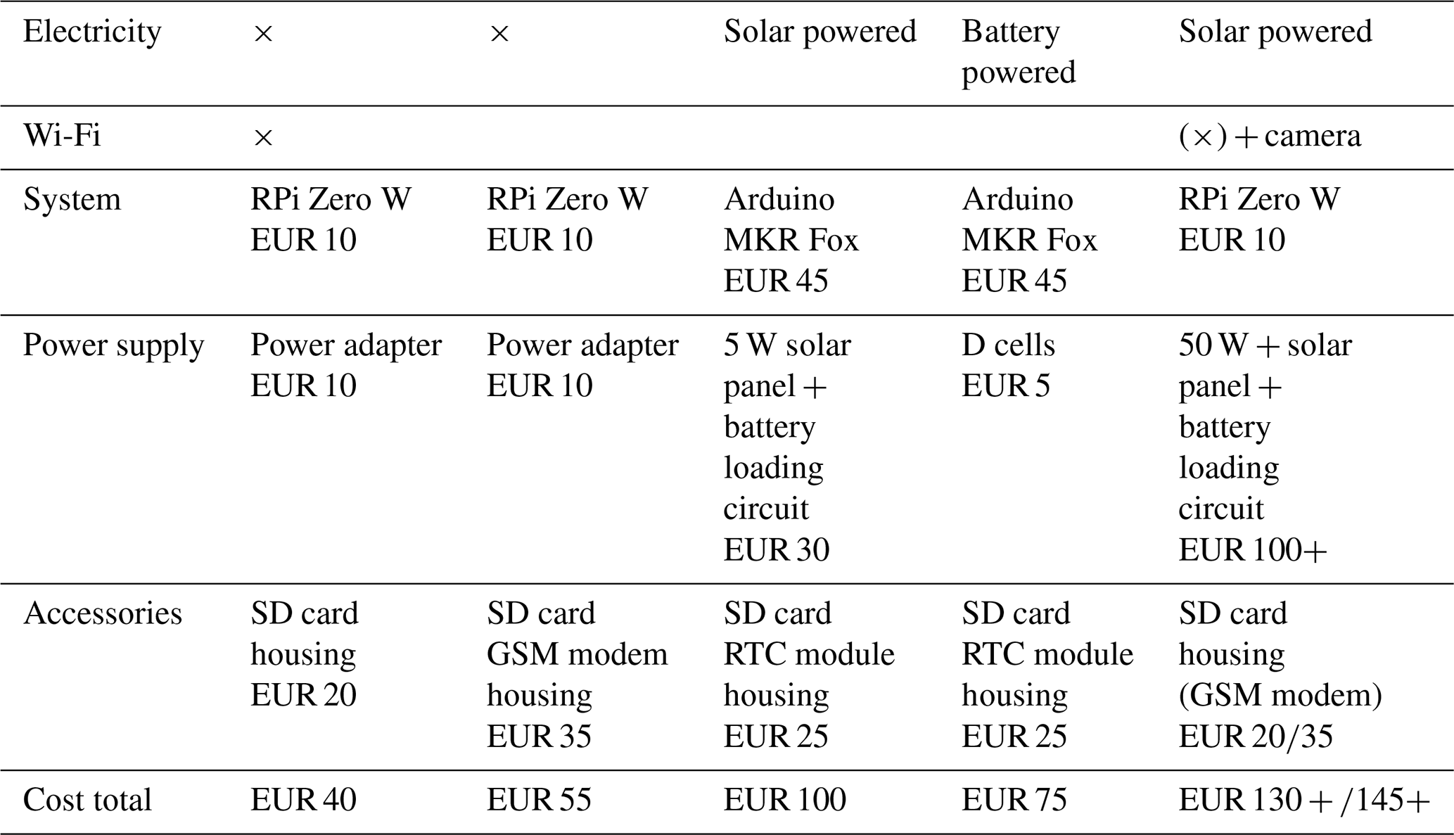
2.2.3 System cost
In this study, the cost for the cheapest monitoring solution is the described RPi option that is powered through the mains while transferring the measured data via Wi-Fi (about EUR 40 + sensors). The cheapest off-grid solution (a system based on Arduino MKR Fox 1200) costs about EUR 75 + sensors. A detailed summary of the system configurations and corresponding costs is given in Table 1.
Table 1Cost for different sensor systems depending on the use case.
2.2.4 Low-cost environmental sensors
The developed systems are capable of connecting to a variety of low-cost sensors (e.g. the temperature/humidity sensors DHT22 and SHT31). In this study, a Bosch BME280 weather sensor (i.e. temperature, humidity, and air pressure) and the semi-professional Davis Vantage Pro2 rain gauge had been used for demonstration. Furthermore, a RPi-based system has been used in conjunction with a SHT31 temperature/humidity sensor, a pyranometer, and a Davis Vantage Pro2 rain gauge. The source code for those setups is available through Zenodo (Krüger, 2024a).
2.2.5 Low-cost rain gauge
The considered rain gauge uses the tipping bucket principle. It consists of a collector cone with a spherical opening at the top. The collected precipitation is lead through a debris-filtering screen into a container with two buckets on a pivot. When one bucket fills up with water, it eventually tips and empties the container, bringing the other bucket in position to be filled. Each time the bucket tips, a contact is triggered which can be counted by a connected microcontroller or sensor system.
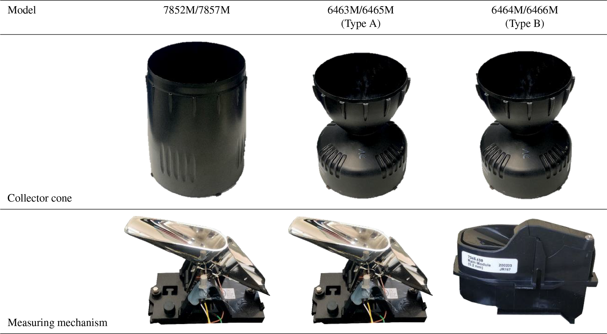
Within the time frame of this study, the design of the Davis rain gauge has been altered by the manufacturer. In particular, three different models were available in that time frame. In the first update, the design of the upper part (collector cone) of the device changed. While the old version (model no. 7852M/7857M) had the shape of a truncated cone, the new one (model no. 6463M/6465M; further referenced as Type A) has the shape of a funnel inside the cone. After the field study described in the next chapter, the design (model no. 6464M/6466M; further referenced as Type B) was changed again. This time, the tipping mechanism changed from a two-bucket design to a one-bucket design. Instead of tipping and bringing the second bucket into position, the new design uses a counterweight that returns the bucket to the collection position after emptying upon reaching the given amount of precipitation. The three types can be seen in Table 2. As the older types are still widely in use, the results of this study still apply for a wide range of users.
Table 2Different versions of the used low-cost rain gauge. The collector cone and measuring mechanism changed over time.
2.3 Quality assessment of a low-cost rain gauge
To benefit from the use of low-cost sensors, these have to provide a certain level of data quality and reliability. Thus, these properties have to be assessed and verified for a given sensor type. Two goals were pursued with regard to the performance assessment. On the one hand, the accuracy of the rain gauge was assessed. On the other hand, the quality (spread) of the factory calibration and thus the suitability in a low-cost, out-of-the-box use case was examined. Therefore, two studies have been performed which will be described in the following sections.
2.3.1 Lab calibration
To assess the quality of the factory calibration, a static calibration was carried out (Marsalek, 1981). Hereby, the volume of water which is required to tip the bucket is measured using a syringe and a microscale.
The calibration was carried out in the lab for 37 new tipping gauges of Type A. Furthermore, 20 rain gauges of the same type used in the field study were also examined directly at site, i.e. lab-calibrated on site, after carrying out the field study. As the manufacturer changed the design after the completion of the field study, another lab calibration with nine new gauges of Type B was carried out.
In preparation for the lab calibration, the table was levelled utilising adjustable screws on the table legs. The rain gauges themselves have been levelled using a built-in bubble level. Furthermore, slices of paper have been used to account for the remaining unevenness on the table. During the calibration, all gauges were oriented in exactly the same direction on the table. All measurements were taken using a G&G microscale with an accuracy of 0.01 g. The rain collector has a diameter of 16.5 cm, which equals to 4.277 mL or 4.269 g of water (Tanaka et al., 2001) for each tipping of the bucket, i.e. after 0.2 mm rainwater has been collected, as stated by the manufacturer. For each gauge, the following process was executed 20 times:
-
calibrating the microscale using a 100 g calibration weight;
-
weighing an arbitrarily chosen amount of water (4–7 g) on the microscale;
-
drawing up water into a syringe directly from the scale;
-
dripping water slowly into one chamber of the tipping bucket (starting on the side of the pole mount) until the bucket tips;
-
clearing the remaining water in the syringe back onto the microscale and subsequently taking a weight measurement;
-
calculating the difference between the two measurements;
-
removing the remaining water in the bucket using a paper towel; and
-
going back to step 2.
Each weighing side was triggered 10 times (for models 6463M/6465M) to minimise the influence of random measurement inaccuracies. In addition to calculating the weight differences, an iterated mean value of these differences was calculated. The deviation of this iterated mean value from the mean value after 10 measurements provides information about the number of measurements after which the mean value calculated up to that point is stable, i.e. converged. This value can help estimate how many measurements are necessary to make a reliable statement about the weighing properties of the precipitation tipping buckets. Furthermore, the obtained mean allows statements on absolute accuracy to be made. According to the manufacturer, the expected value is 0.2 mm. Deviations from this value show whether over- or undercatch is to be expected in the precipitation measurement.
2.3.2 Field study
A field study was carried out at the meteorological site of the TU Dresden (Dresden University of Technology). The site is situated in the valley of the river Wilde Weißeritz (50°59′ N, 13°35′ E; altitude 220 m NN (height above Amsterdam Ordnance Datum (NAP)); average annual precipitation in the period 1981/2010 was 795.4 mm; Chair of Meteorology, 2023). Several different professional instruments are measuring precipitation here, including a traditional Hellmann rain gauge, an OTT Pluvio gauge, and a Young tipping gauge. These instruments are regularly maintained to meet the specifications of the World Meteorological Organization (WMO).
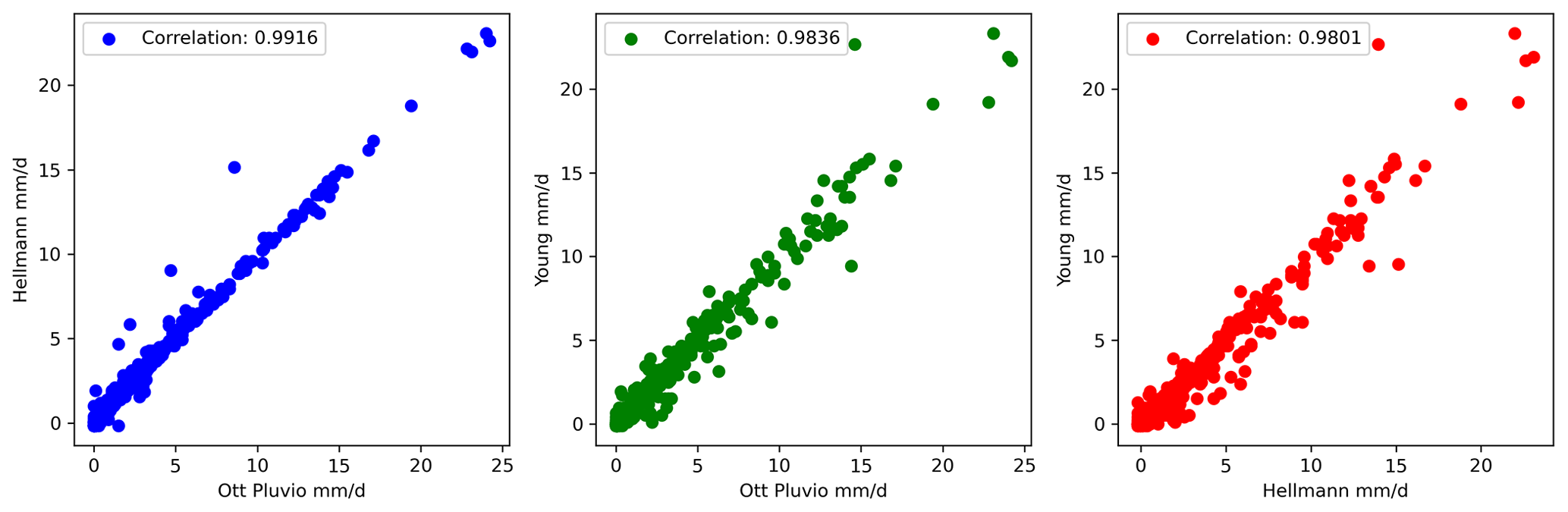
Figure 1Scatterplots for the combinations of the three professional gauges depicting daily precipitation values for 2017 to 2019.
The Hellmann gauge is made of a steel cylinder and has a collecting area of 200 mm2. The collected water runs through a funnel into a small container which is emptied daily at 07:00 CET, and the amount of water in the container is measured to calculate the precipitation for the last 24 h. The Hellmann device has been used as the reference for the climatological measurements taken at this station since 1951 (Fig. 2) and is thus considered the reference instrument in this study. The Hellmann gauge requires no mechanical and electronic parts; thus, the data quality should be stable as the instrument has been set up properly.
The OTT Pluvio is a weighing rain gauge consisting of a collector cylinder (collecting area of 200 mm2) and weighing cell. The weight of the water collected in the cylinder is weighed constantly, and subsequently, a precipitation amount for each minute is generated. The resolution of the precipitation data is 0.1 mm.
The third professional device is a Young tipping gauge that utilises the same measurement principle as the low-cost gauge, i.e. using a tipping bucket. The Young gauge also has a collecting area of 200 mm2, and it has a measurement resolution of 0.1 mm per tip. In contrast to the low-cost gauges, this device is equipped with a heating, which allows snow precipitation to be measured.
Even with three professional gauges, the true precipitation remains unknown as each of these devices is also associated with uncertainties. Triple collocation analysis (Stoffelen and Vogelzang, 2012; Stoffelen, 1998) can be used to estimate the error variances of these three independent but collocated data sets without requiring knowledge of the true precipitation amount. We used a longer time series of the three professional gauges lasting 3 years (from 1 January 2017 to 31 December 2019), consisting of daily observations, to estimate the uncertainties. Inspection of the three scatterplots (Fig. 1) with all combinations of reference gauges led to the assumption that the OTT Pluvio is the best performing because the scatterplots for the Hellmann and Young devices revealed lower correlations (Stoffelen and Vogelzang, 2012). Therefore, we used an implementation provided by Jur Vogelzang (https://github.com/knmiscat/triple_collocation, last access: 3 January 2024) to estimate the error variances with the OTT Pluvio as a reference system. Subsequently, the daily error standard deviations (SDs) could be determined as follows: SDPluvio = 0.150 mm d−1, SDHellmann = 0.183 mm d−1, and SDYoung = 0.278 mm d−1. These values were used to evaluate the results of the low-cost gauges when compared with the reference gauges.
The setup of the study was chosen to enable the analysis of the spread of measurements relying on the factory calibration. Therefore, an array of 20 identical, new, low-cost rain gauges of Type A were set up. The rain gauges were mounted on a wooden frame in an array of four by five devices, covering an area of about 1 m2. The frame is levelled and set at a height of about 1 m above ground to match to the height of the reference gauges located about 10 m to the south of the reference instruments. The horizontality of the rain gauges was ensured by the usage of the built-in bubble level of the rain gauges and the washers while fixing the gauges to the (levelled) frame. The setup is shown in Fig. 2. A Raspberry Pi (RPi Model 3b) sensor system is used to log the precipitation data (i.e. timestamps of tipping events) of the rain gauges. To compare the low-cost gauge measurements with the reference instruments, the number of tipping events is multiplied by 0.2 mm per tipping, as stated by the manufacturer. The time synchronisation of the low-cost sensor system with the reference gauges was ensured by setting the time for both type of systems through the network time protocol (NTP). Cumulative rainfall was measured in the months from August 2018 to April 2019.
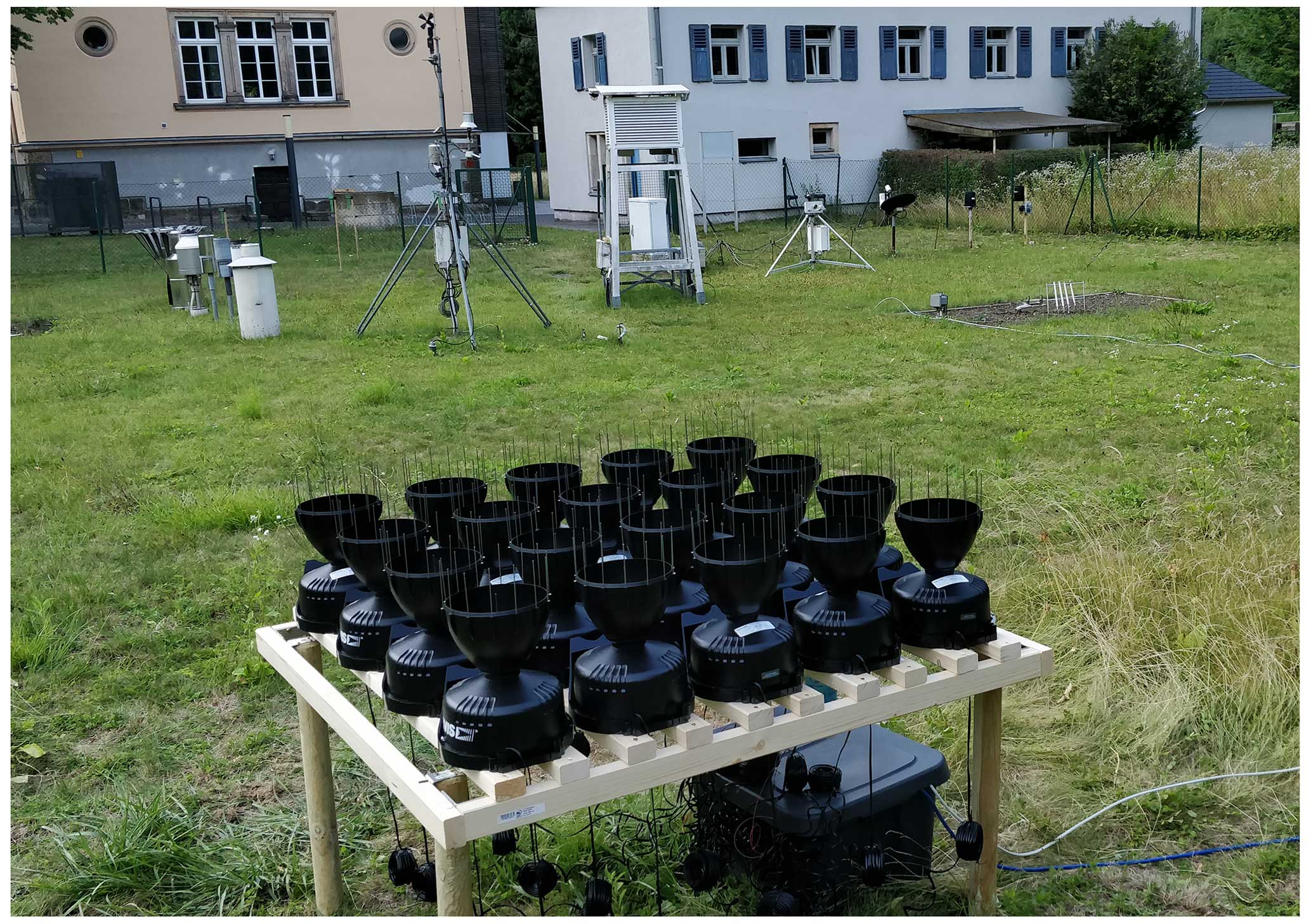
Figure 2Tharandt meteorological site with reference instruments (in the background on the left-hand side) and field study setup (in the foreground).
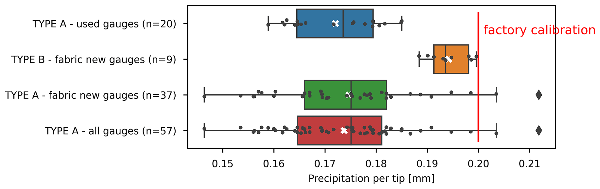
Figure 3Comparison between used and new gauges with respect to precipitation needed per tip. The mean for each group depicted with a cross. The factory calibration claimed by manufacturer is shown with a red line.
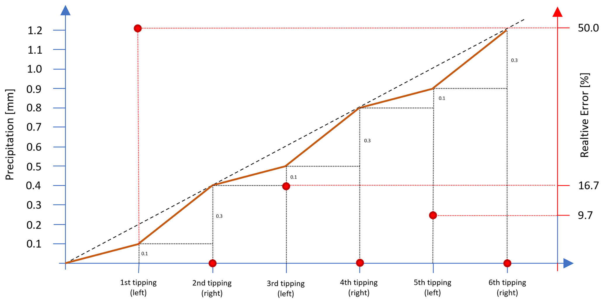
Figure 4Development of relative errors due to difference between the left and right tippings. The relative error decreases with each consecutive tipping within a rain event (error is shown with red dots, from left to right; cumulative precipitation is shown with a red line).
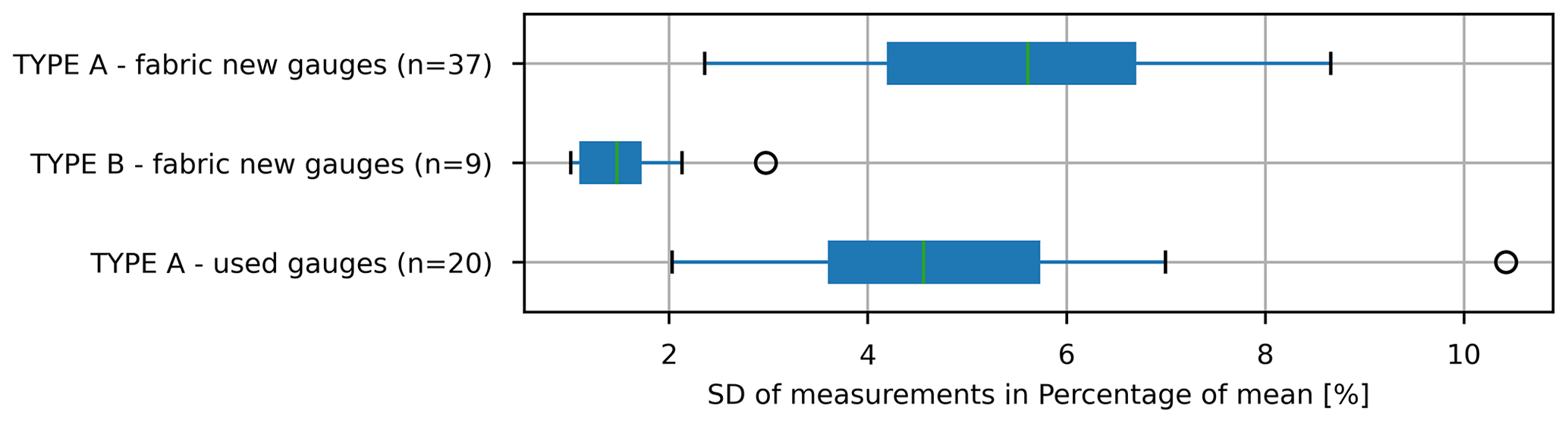
Figure 5Comparison between used and new gauges. The SD of single measurements is given as a percentage of the mean.
3.1 Lab calibration
In total, 66 rain gauges have been tested. Of these devices, 37 were new gauges of Type A and 20 had already been used for about half a year (i.e. in the field study; Type A). A further nine gauges used the new single tipping bucket mechanism (Type B). None of the gauges had been recalibrated before (Krüger, 2024a).
Considering all rain gauges of Type A, the mean water amount required for one tip was 0.174 mm with a standard deviation of 0.013 mm. The mean value for new gauges was 0.175 mm (SD 0.014 mm), and for the used gauges, it amounted to a mean of 0.172 mm (SD 0.009 mm) (Fig. 3). In contrast, the amount of water required for one tip for the gauges of Type B was 0.194 mm with a standard deviation of 0.004 mm. The distribution of results in all four groups (A – new, A – used, and A – all; B) was tested to see if it is Gaussian using the Kolmogorov–Smirnov test (α=0.05). This could be confirmed for all four groups.
Confidence intervals for a level of 95 % have been calculated as follows: A – new (0.1680–0.1795 mm); A – used (0.1699–0.1795 mm); A – all (0.1704–0.1771 mm); and B (0.1911–0.1972 mm).
The measured average rain amount to tip the bucket is lower than the stated value of the manufacturer (0.2 mm) for both types, although the average of Type B is only off by 2.9 % compared to −13.2 % for Type A. The measurements in the laboratory were taken without the rain collector and thus are not accounting for loss effects of evaporation and wind.
The measurements of both Type A groups (used and new gauges) show large differences between the left- and right-hand side of the tipping bucket. This leads to larger errors for small precipitation events (Fig. 4). Nevertheless, the influence of the different sensitivities of the respective left and right sides decreases continuously with an increasing number of tips during a precipitation event and eventually approaches the mean value of all left and right tips of the gauge. To minimise this influence, Marsalek (1981) states that a standard deviation of smaller than 2 % of the mean is desirable; no gauge of Type A could satisfy this need.
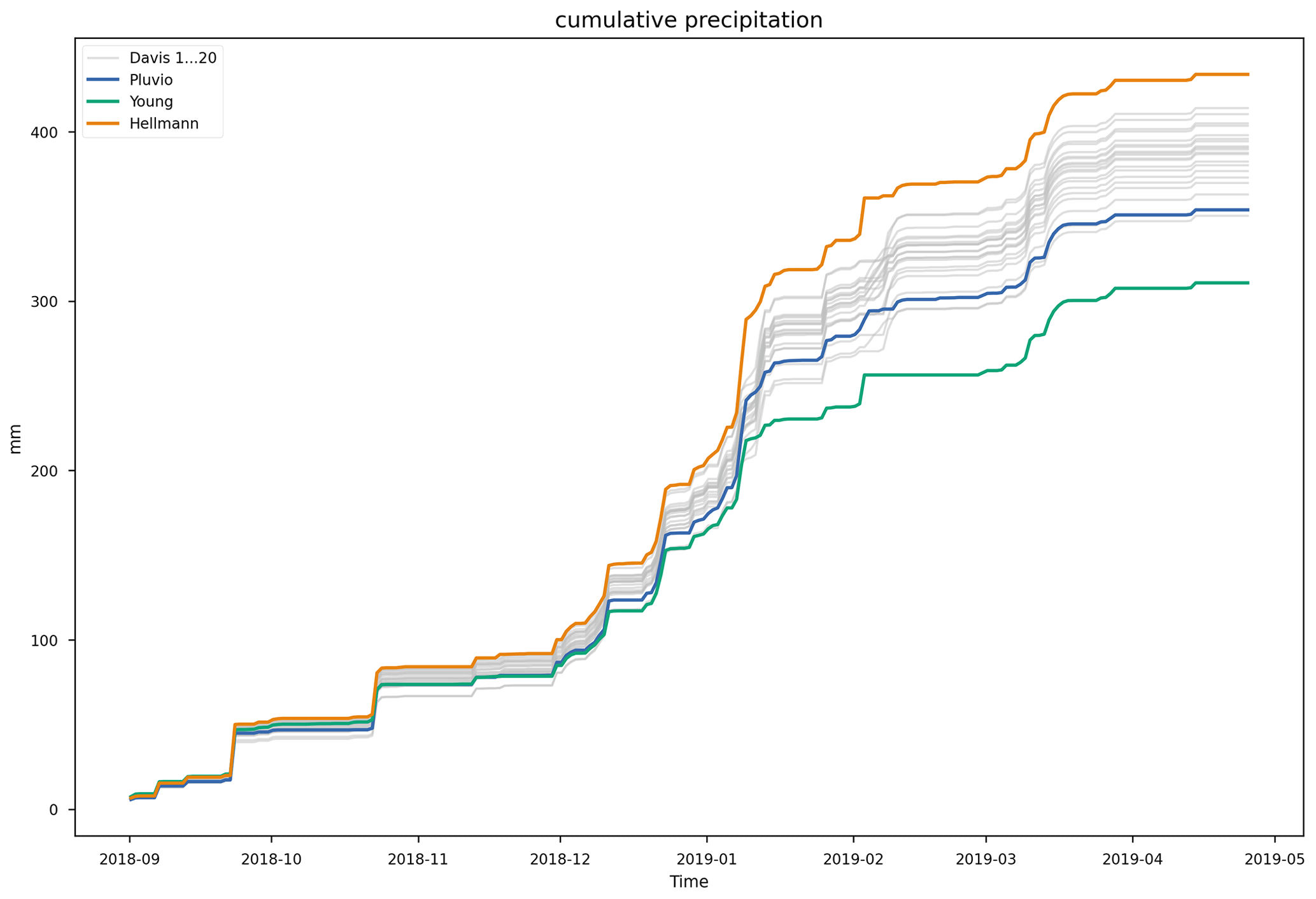
Figure 6Cumulative precipitation for all low-cost gauges and three professional gauges for the whole study time.
Although no bias due to tipping bucket sides is an issue for Type B, differences between individual measurements still exist. However, this variation is much smaller than the differences which could be observed within the Type A group. While the average SD of the single measurements for Type A gauges was 5.6 % (new) and 4.7 % (used) of the mean, it was only 1.6 % for Type B gauges (see Fig. 5). Seven out of nine tested gauges of Type B fulfilled the threshold of 2 % stated by Marsalek (1981).
3.2 Field study
Precipitation data were collected for the period from 1 August 2018 to 30 April 2019. As there were some gaps in the data for the professional gauges in August 2018 and at the end of April 2019, the data for the whole data set were analysed for the period from 1 September 2018 to 25 April 2019. Additionally, there were rare occurrences of gaps in the time series of the Young tipping gauge (28 October 2018 and 21 and 28 February 2019) which could not be explained. Those days have been removed from the data set for all gauges.
Figure 6 shows the plot of cumulated precipitation for the whole investigation period. The Type A rain gauges show on average less underestimation (385.85 mm; −11.1 %, SD = 17.0 mm) than the other automatic rain gauges when compared to the Hellmann gauge (433.9 mm). While the results of the OTT Pluvio gauge are slightly worse than the results of the low-cost gauges (353.9 mm; −18.4 %) the results of the Young tipping gauge are considerably worse than the low-cost gauges (310.8 mm; −28.4 %).
The measured sums of the 20 low-cost gauges range from 350.4 mm, which is slightly less than the OTT Pluvio gauge, to 414.0 mm, which is slightly less than the sum of collected precipitation of the Hellmann gauge. The distribution of the measurements of the low-cost gauges compared to the professional gauges is shown in Fig. 7.
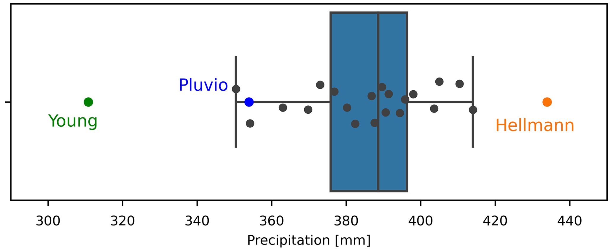
We used the obtained daily error standard deviations (see Sect. 2.3.2) to run a Monte Carlo simulation (n=100) with the daily time series for each professional gauge to obtain a synthetic distribution of the cumulated values for each gauge. These distributions were compared with the distribution of the 20 low-cost gauges utilising a t test. This resulted in a rejection of the null hypothesis for all professional gauges. Thus, all reference gauges are significantly outside of the distribution of low-cost gauges.
Part of the variation in the results of the low-cost gauges can be explained by the lack of recalibration prior to their usage. In the lab analysis, calibration values between 0.159 and 0.185 mm were obtained, which correspond to a range between −7.6 % and +7.6 % of the mean of all gauges. This is in the same range as the measured precipitation (−9.3 % to +7.6 % of the mean of all gauges). Nevertheless, calibration values and observed precipitation totals show only a moderate negative correlation Fig. 8. For example, gauge 14 recorded the lowest number of tips, and its correlation value (amount of water needed per tip) was the highest. In contrast, gauge 10 and gauge 13 measured about the same amount of precipitation (tippings), but their calibration values are in completely different ranges.
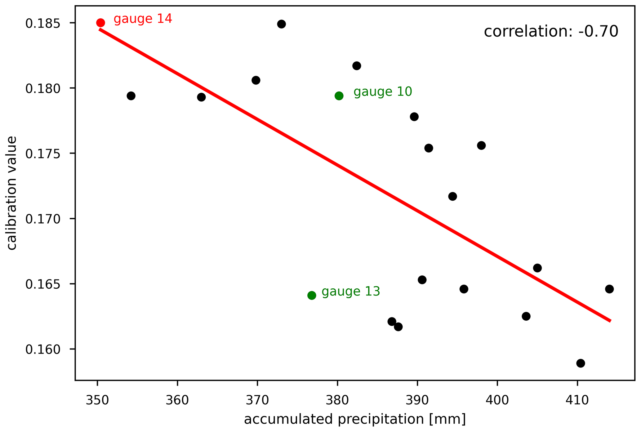
Figure 8Calibration values vs. measured precipitation of the 20 gauges used in the field study (Type A).
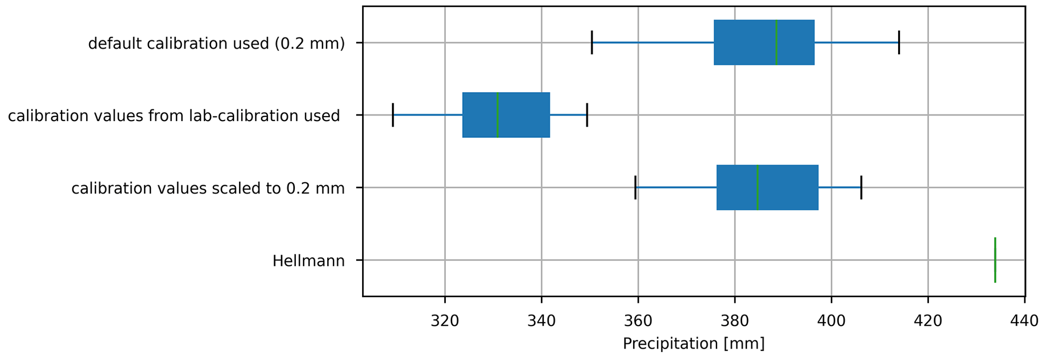
Multiplying the calibration values of each gauge with the tippings recorded by the associated gauge would result in a much lower measured precipitation (due to the lower mean of 0.172 mm). However, the standard deviation would also be much smaller (12.5 mm vs. 17.5 mm; Fig. 9). Thus, to improve the issue of the scattered calibration values, one could then scale the mean of the calibration values to the claimed value by the manufacturer of 0.2 mm and subsequently all values by this factor. This would then result in a higher precision of the obtained precipitation for all gauges. Nevertheless, this step is only possible for a larger group of gauges at hand.
Comparing the cumulated rainfall values of the different gauges in more detail, two periods of strong deviations of the low-cost gauges to the professional gauges can be seen. This observation can be made for all low-cost gauges and is caused by partial blocking of the funnel with snow on 8 January and 3 February 2019 (see Fig. 10 which shows the cumulative rainfall with an hourly resolution). On 8 January 2019, rising temperatures led to simultaneous snow melting in all gauges and a subsequent run off and registration of the melting snow on 12 January 2019 and on the following days. On 3 February 2019, a warming of the black funnel due to solar irradiation led to a slightly different pattern of precipitation measurement. This time, the gauges at the edge of the array were emptied first (nos.1–5, 10, 15, and 20), while the ones inside the array were blocked for longer (e.g. nos.6–9, 11–14, and 16–19) until 8 February 2019.
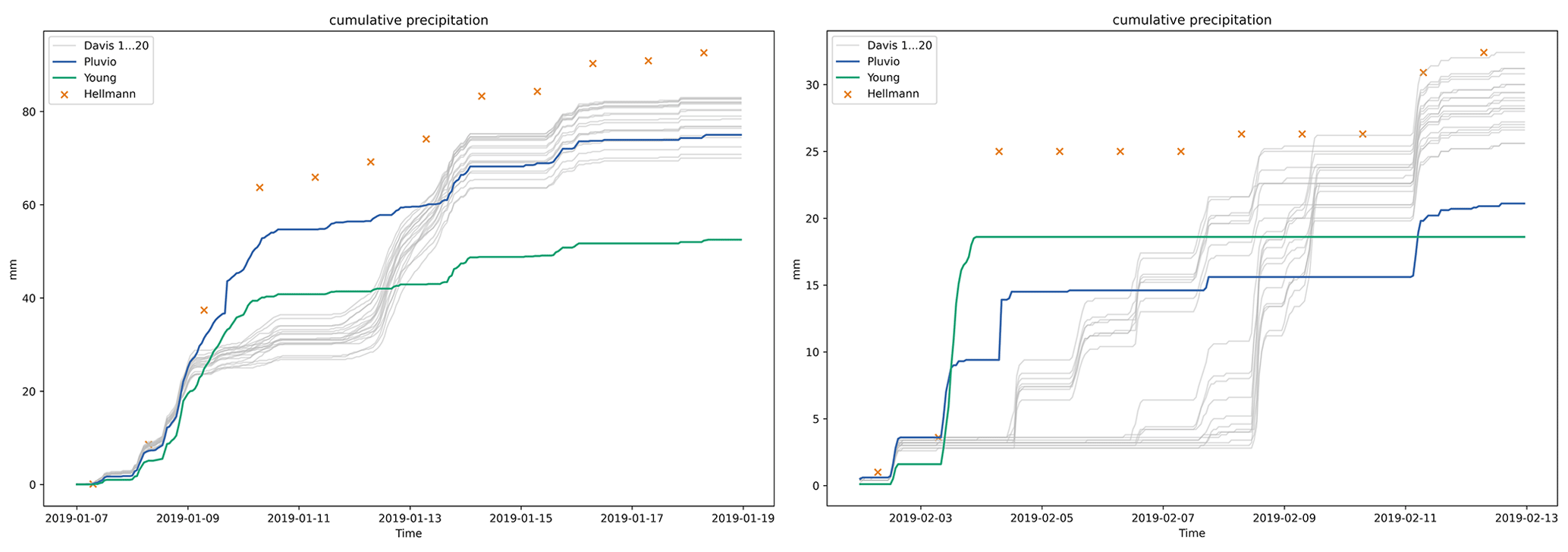
Figure 10Cumulative rainfall for two selected periods with hourly resolution. Note that hourly data for the Hellmann gauge are not available and hence are only marked with the daily readings (orange crosses).
Although the results of the cumulative precipitation over the whole testing period are promising, the Pearson correlation coefficient values for shorter time frames are not. The correlations for daily values between the different low-cost gauges are high (0.937 … 0.997). However, the correlations with the professional gauges are significantly lower (0.779–0.841 for Hellmann, 0.730–0.784 for Young, and 0.828–0.890 for OTT Pluvio). The low-correlation values can partly be explained by the circumstance that the low-cost gauges have no heating to handle snow precipitation. Removing the days with blockages and the subsequent melting of water from the data set (9–15 January/3–10 February) yields a strong increase in the correlation values (daily) with the professional gauges (0.973–0.990 for Hellmann, 0.897–0.912 for Young, and 0.973–0.991 for OTT Pluvio). Nevertheless, correlation values within the group of low-cost gauges are higher compared to the professional gauges, ranging from 0.977 to 0.999 for daily values.
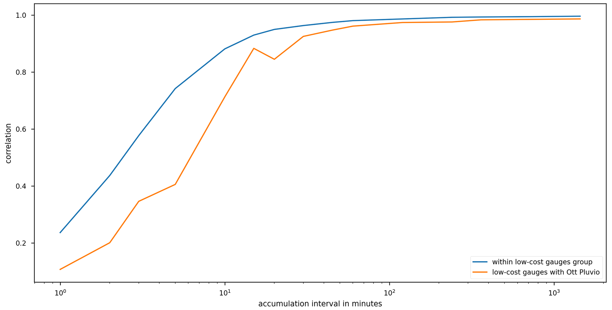
Figure 11Average correlation values for different accumulation intervals (low-cost vs. low-cost and low-cost vs. OTT Pluvio).
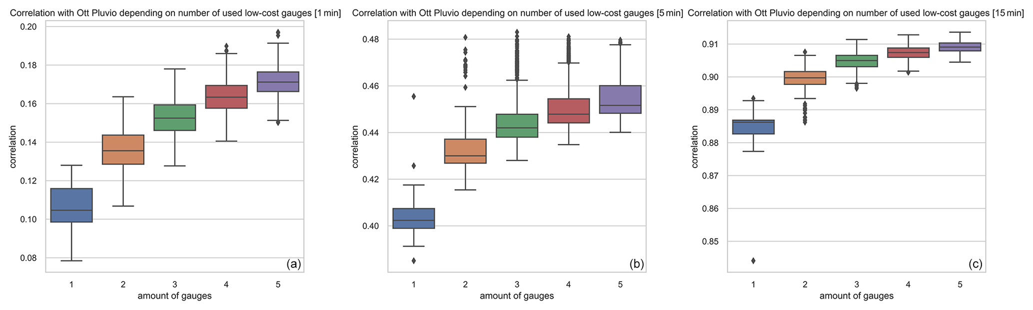
Figure 12Correlation for average rainfall measured by subset of 1–5 low-cost gauges with OTT Pluvio for three different accumulation intervals at (a) 1 min, (b) 5 min, and (c) 15 min.
Measuring principles (weighing vs. tipping gauge) and resolutions (0.1 mm vs. 0.2 mm) differ between OTT Pluvio and the low-cost gauges. Therefore, correlation values were calculated for a wide range of accumulation intervals (1 min to 1 d) to assess which accumulation intervals might be needed for acquiring reliable data. As expected, correlations increase with an increased accumulation time. As already shown for the daily values, correlations within the group of low-cost gauges are higher than correlations between low-cost gauges and OTT Pluvio. Nevertheless, differences decrease with increasing accumulation intervals (Fig. 11).
As the correlation of the low-cost gauge with OTT Pluvio is very low for accumulation intervals of 15 min and shorter, one could try to use several low-cost rain gauges to overcome this problem. We investigated this by randomly choosing a subset of gauges (1 to 5) from the data set and subsequently calculating the correlation of their average measurement with the reference gauge for 2000 simulations. Results for 1, 5, and 15 min can be seen in Fig. 12. It can be shown that an increase in the used gauges leads to increased correlations. The biggest gain can be seen when changing from one to two gauges. The effect than diminishes with further gauges. Nevertheless, the benefit of added gauges is a lot smaller compared to increasing the accumulation interval.
In this study, we assessed the suitability of a widely used low-cost precipitation sensor for an out-of-the-box use, i.e. applying the sensor in the field without prior calibration. The results of the lab calibration suggest that it is beneficial to check the factory calibration for the older type of the sensor (Type A) for outliers.
4.1 Lab calibration
It could be shown for Type A gauges that the mean of two consecutive tippings is consistent across all tested gauges resulting in a mean of 0.174 mm per tip. However, it also became obvious that some tipping gauges deviated strongly from this mean value. Utilising the presented analysis scheme outliers from the expected mean can be detected after approximately four to five tilts per side. Furthermore, the amount of water required for a tipping of one of the buckets is important. In the case of large differences between both bucket sides, the measurement accuracy of very small precipitation events, in which only a few tilts occur, will be affected more strongly, resulting in larger relative errors. However, this is only the case for odd numbers of tipping. A recalibration of the gauge is recommended if the difference between both bucket sides is larger than 0.05 mm of precipitation (25 % of nominal volume). In contrast, Marsalek (1981) advised continuing the calibration until the mean was within of 2 % of the nominal volume.
The measured means of the tipping are consistently lower than 0.2 mm across all gauges (Types A and B), leading to the assumption that a factory calibration might have been performed. Furthermore, potentially only one side of the mechanism (Type A only) had been calibrated until the desired volume was met, which could have led to the observed differences between the two buckets. Due to the design of a tipping bucket, water is lost when the bucket is tilted, as the other bucket is not in position again fast enough. This can lead to an undercatch which increases with the rainfall intensity. These errors can range from 10 % to 30 % (Humphrey et al., 1997; Marsalek, 1981). Furthermore, error influences due to evaporation and wind are conceivable.
In contrast to the results of gauges of type A, the measured mean for Type B (0.194 mm) is considerably closer to the nominal volume (0.2 mm). Also, the deviations between the single measurements are much smaller compared to Type A. These gauges might have been factory calibrated to a higher volume because the mechanism is less prone to undercatch at higher-rainfall intensities.
4.2 Field study
In the field study, it could be shown that the gauges of Type A, on average, show accumulated rainfall results which are closer to the Hellmann reference gauge than the two other professional gauges. Nevertheless, the spread of the measured precipitation totals is about twice as big as that stated in the manufacturer's data sheet (±4 %), with deviations ranging from −9.3 % to +7.6 % compared to the mean of all gauges. Even the SD for all gauges (4.6 %) is bigger than that value. The manufacturer is stating that this accuracy is valid for rain rates up to 100 mm h−1, which have not been observed by any of the gauges in the study period.
Parts of this variability can be explained by the lack of calibration before use, as shown above.
Furthermore, other error sources can have an impact on the measured precipitation. As the 20 gauges have been placed in a very dense array, some of the gauges are more shielded from the wind compared to others. This should lead to an undercatch for the exposed gauges when compared to the more shielded ones (Pollock et al., 2018). Nevertheless, this systematic behaviour was not observed.
Splashing of raindrops and thus rainfall being diverted to adjacent gauges might lead to a systematic pattern in the dense array. However, this was not observed in this study.
The dense array could have an influence on evaporation behaviour, as some gauges are more exposed to direct sunlight than others. This is especially true in the winter months, as the Sun only rises to very low angles, which was already seen in the behaviour of the melting snow (as described above).
A further source of error might also be the non-optimal mount of the gauges. To ensure good readings, the gauges have to be perfectly levelled (Burt, 2009). While installing the array, the levelling was done using the provided circular bubble level, which has limited accuracy. Furthermore, the frame on which the gauges were installed was made of wood, which might degrade and thus move over time.
Last, but not least, although the array only covered an area of about 1 m2, small-scale variability in the rain fields could also play a role when obtaining different precipitation readings. Nevertheless, other studies, e.g. the WMO field intercomparison of rain intensity gauges (Lanza and Vuerich, 2009), used similar or bigger sized setups to this study.
In this study, two low-cost sensor systems based on the Arduino and Raspberry Pi families have been presented. Here it could be shown that utilising widely available open-source hardware allows the user to flexibly create a sensor system tailored to their needs on a given site while keeping the costs low. The presented systems are capable of logging sensor data of various sensors and are able to either log data locally or transmit the data to the internet.
Furthermore, the factory calibration of the widely used Davis tipping rain gauge was examined, both in the laboratory and in the field. In the lab, different generations of the gauge have been tested. Here, the results show a distinct difference between the old and the newer generation of the gauge. While for the older type an average of 0.174 mm of water was needed for a tip, 0.194 mm was needed for the newer generation, which is less than the amount officially stated by the manufacturer. For the older type, it was also found that the gauges are not tipping equally with both buckets. This leads to errors in the precipitation measurements for small rain events. To minimise this error, gauges should be checked and calibrated for equal tipping before installation. This is particularly important for the several tens of thousands of gauges of Type A probably already in use worldwide. Here, the factory calibration should at least be checked. For the newer Type B, it could be found that the deviation between the tippings is much smaller compared to the old type. Whether this has a positive impact on the accuracy was not within the scope of this study but has to be further investigated. Nevertheless, for these gauges, the factory calibration should also be checked before use, as our sample was very small (n=9).
Beside the lab calibration, 20 gauges (Type A) have been tested against professional rain gauges in the field. Here, the results showed an undercatch when compared to the reference Hellmann gauge of the climate station where the array was installed. Furthermore, it could be shown that the spread of the factory calibration is larger (by a magnitude of 2) than stated by the manufacturer. Nevertheless, the results of the low-cost gauge were closer to the reference than the Young tipping gauge and OTT Pluvio, respectively. Our results suggest (high correlation for longer accumulation intervals vs. professional gauges) that the error due to undercatch could be mitigated by applying a factor for each gauge; however, this would require measurements against a reference station either in the field or in the lab.
The study has shown that the tested low-cost sensor is suitable for use in the collection of meteorological data. However, the factory calibration should at least be checked, if not recalibrated, before use. When paired with a low-cost sensor system and properly set up, these sensors can be beneficial for the densification of existing sensor networks. For accurate results, the desired out-of-the-box use is not recommended.
Data sets obtained during the experiments (lab and field), as well as source code, are available from Zenodo at https://doi.org/10.5281/zenodo.10838614 (Krüger, 2024a). The source code will be updated and is available on GitHub (https://github.com/kruegertud/tharandt_raingauge/, Krüger, 2024b).
RK and PK developed the concept and methodology for the study. RK programmed the code for the sensor systems and carried out the investigation and subsequent formal analysis. PK supported by setting up and by carrying out the experiments. RK created the visualisations and wrote the original draft of this paper. PK and AE reviewed the paper and gave continuous support during the study.
At least one of the (co-)authors is a member of the editorial board of Geoscientific Instrumentation, Methods and Data Systems. The peer-review process was guided by an independent editor, and the authors also have no other competing interests to declare.
Publisher's note: Copernicus Publications remains neutral with regard to jurisdictional claims made in the text, published maps, institutional affiliations, or any other geographical representation in this paper. While Copernicus Publications makes every effort to include appropriate place names, the final responsibility lies with the authors.
We would like to express our gratitude to the Institute of Hydrology and Meteorology at TU Dresden for granting us the opportunity to conduct our field study on their meteorological site, as well as for their continuous support throughout the measuring campaign.
This open access publication was financed by the Saxon State and University Library Dresden (SLUB Dresden).
This paper was edited by Ralf Srama and reviewed by Rolf Hut and one anonymous referee.
Adla, S., Rai, N. K., Karumanchi, S. H., Tripathi, S., Disse, M., and Pande, S.: Laboratory Calibration and Performance Evaluation of Low-Cost Capacitive and Very Low-Cost Resistive Soil Moisture Sensors, Sensors, 20, 363, https://doi.org/10.3390/s20020363, 2020.
Blanch, X., Abellan, A., and Guinau, M.: Point Cloud Stacking: A Workflow to Enhance 3D Monitoring Capabilities Using Time-Lapse Cameras, Remote Sens., 12, 1240, https://doi.org/10.3390/rs12081240, 2020.
Brown, S. L., Goulsbra, C. S., Evans, M. G., Heath, T., and Shuttleworth, E.: Low cost CO2 sensing: A simple microcontroller approach with calibration and field use, HardwareX, 8, e00136, https://doi.org/10.1016/j.ohx.2020.e00136, 2020.
Burt, S.: The Davis Instruments Vantage Pro2 wireless AWS – an independent evaluation against UK-standard meteorological instruments, https://www.weatherstations.co.uk/wp-content/uploads/Prodata-Expert-Guide-No.-1-Davis-VP2-AWS-c-Stephen-Burt-2009.pdf (last access: 4 June 2024), 2009.
Chair of Meteorology: Tharandt Klimastation, https://tu-dresden.de/bu/umwelt/hydro/ihm/meteorologie/forschung/mess-und-versuchsstationen/tharandt-klimastation?set_language=de (last access: 10 May 2023), 2023.
de Vos, L., Leijnse, H., Overeem, A., and Uijlenhoet, R.: The potential of urban rainfall monitoring with crowdsourced automatic weather stations in Amsterdam, Hydrol. Earth Syst. Sci., 21, 765–777, https://doi.org/10.5194/hess-21-765-2017, 2017.
Dini, B., Bennett, G. L., Franco, A. M. A., Whitworth, M. R. Z., Cook, K. L., Senn, A., and Reynolds, J. M.: Development of smart boulders to monitor mass movements via the Internet of Things: a pilot study in Nepal, Earth Surf. Dynam., 9, 295–315, https://doi.org/10.5194/esurf-9-295-2021, 2021.
Eltner, A., Elias, M., Sardemann, H., and Spieler, D.: Automatic Image-Based Water Stage Measurement for Long-Term Observations in Ungauged Catchments, Water Resour. Res., 54, 10362–10371, https://doi.org/10.1029/2018WR023913, 2018.
Eltner, A., Bressan, P. O., Akiyama, T., Gonçalves, W. N., and Marcato Junior, J.: Using Deep Learning for Automatic Water Stage Measurements, Water Resour. Res., 57, e2020WR027608, https://doi.org/10.1029/2020WR027608, 2021.
Fraga, I., Alvarellos, A., and González-Coma, J. P.: Exploring the Feasibility of Low Cost Technology in Rainfall Monitoring: The TREBOADA Observing System, in: The 2nd XoveTIC Conference (XoveTIC 2019), XoveTIC Conference, 5–6 September 2019, A Coruña, Spain, https://doi.org/10.3390/proceedings2019021005, 2019.
Gamperl, M., Singer, J., and Thuro, K.: Internet of Things Geosensor Network for Cost-Effective Landslide Early Warning Systems, Sensors, 21, 2609, https://doi.org/10.3390/s21082609, 2021.
Humphrey, M. D., Istok, J. D., Lee, J. Y., Hevesi, J. A., and Flint, A. L.: A New Method for Automated Dynamic Calibration of Tipping-Bucket Rain Gauges, J. Atmos. Ocean. Tech., 14, 1513–1519, https://doi.org/10.1175/1520-0426(1997)014<1513:ANMFAD>2.0.CO;2, 1997.
Kaspar, F., Müller-Westermeier, G., Penda, E., Mächel, H., Zimmermann, K., Kaiser-Weiss, A., and Deutschländer, T.: Monitoring of climate change in Germany – data, products and services of Germany's National Climate Data Centre, Adv. Sci. Res., 10, 99–106, https://doi.org/10.5194/asr-10-99-2013, 2013.
Krüger, R.: Dataset + SourceCode Final Revision GI Paper, Zenodo [code and data set], https://doi.org/10.5281/ZENODO.10838614, 2024a.
Krüger, R.: tharandt_raingauge, GitHub [code], https://github.com/kruegertud/tharandt_raingauge/ (last access: 4 June 2024), 2024b.
Lanza, L. G. and Vuerich, E.: The WMO Field Intercomparison of Rain Intensity Gauges, Atmos. Res., 94, 534–543, https://doi.org/10.1016/j.atmosres.2009.06.012, 2009.
Lobligeois, F., Andréassian, V., Perrin, C., Tabary, P., and Loumagne, C.: When does higher spatial resolution rainfall information improve streamflow simulation? An evaluation using 3620 flood events, Hydrol. Earth Syst. Sci., 18, 575–594, https://doi.org/10.5194/hess-18-575-2014, 2014.
Lopez, J. C. B. and Villaruz, H. M.: Low-cost weather monitoring system with online logging and data visualization, in: 2015 International Conference on Humanoid, Nanotechnology, Information Technology, Communication and Control, Environment and Management (HNICEM), 9–12 December 2015, Cebu City, Philippines, 1–6, https://doi.org/10.1109/HNICEM.2015.7393170, 2015.
Marsalek, J.: Calibration of the tipping-bucket raingage, J. Hydrol., 53, 343–354, https://doi.org/10.1016/0022-1694(81)90010-X, 1981.
maxim integrated: DS3231 Extremely Accurate I2C-Integrated RTC/TCXO/Crystal, https://www.analog.com/media/en/technical-documentation/data-sheets/ds3231.pdf (last access: 4 June 2024), 2015.
Mendoza-Cano, O., Aquino-Santos, R., López-de la Cruz, J., Edwards, R. M., Khouakhi, A., Pattison, I., Rangel-Licea, V., Castellanos-Berjan, E., Martinez-Preciado, M. A., Rincón-Avalos, P., Lepper, P., Gutiérrez-Gómez, A., Uribe-Ramos, J. M., Ibarreche, J., and Perez, I.: Experiments of an IoT-based wireless sensor network for flood monitoring in Colima, Mexico, J. Hydroinform., 23, 385–401, https://doi.org/10.2166/hydro.2021.126, 2021.
Pollock, M. D., O'Donnell, G., Quinn, P., Dutton, M., Black, A., Wilkinson, M. E., Colli, M., Stagnaro, M., Lanza, L. G., Lewis, E., Kilsby, C. G., and O'Connell, P. E.: Quantifying and Mitigating Wind-Induced Undercatch in Rainfall Measurements, Water Resour. Res., 54, 3863–3875, https://doi.org/10.1029/2017WR022421, 2018.
Rodríguez, B. G., Meneses, J. S., and Garcia-Rodriguez, J.: Implementation of a Low-Cost Rain Gauge with Arduino and Thingspeak, in: 15th International Conference on Soft Computing Models in Industrial and Environmental Applications (SOCO 2020), vol. 1268, edited by: Herrero, Á., Cambra, C., Urda, D., Sedano, J., Quintián, H., and Corchado, E., Springer International Publishing, Cham, 770–779, https://doi.org/10.1007/978-3-030-57802-2_74, 2021.
Singh, D., Sandhu, A., Sharma Thakur, A., and Priyank, N.: An overview of IoT hardware development platforms, Int. J. Emerg. Technol., 11, 155–163, 2020.
Stoffelen, A.: Toward the true near-surface wind speed: Error modeling and calibration using triple collocation, J. Geophys. Res.-Oceans, 103, 7755–7766, https://doi.org/10.1029/97JC03180, 1998.
Stoffelen, A. and Vogelzang, J.: Triple collocation, ResarchGate, https://doi.org/10.13140/RG.2.2.30926.66888, 2012.
Strigaro, D., Cannata, M., and Antonovic, M.: Boosting a Weather Monitoring System in Low Income Economies Using Open and Non-Conventional Systems: Data Quality Analysis, Sensors, 19, 1185, https://doi.org/10.3390/s19051185, 2019.
Sudantha, B. H., Warusavitharana, E. J., Ratnayake, G. R., Mahanama, P. K. S., Warusavitharana, R. J., Tasheema, R. P., Cannata, M., and Strigaro, D.: 4ONSE as a complementary to conventional weather observation network, in: 2019 4th International Conference on Information Technology Research (ICITR), 10–13 December 2019, Moratuwa, Sri Lanka, 1–6, https://doi.org/10.1109/ICITR49409.2019.9407798, 2019.
Tanaka, M., Girard, G., Davis, R., Peuto, A., and Bignell, N.: Recommended table for the density of water between 0 °C and 40 °C based on recent experimental reports, Metrologia, 38, 301–309, https://doi.org/10.1088/0026-1394/38/4/3, 2001.