The Harwell TCCON observatory

The Harwell observatory, located in Oxfordshire, UK (51.571° N, 1.315° W), now part of the Total Carbon Column Observing Network (TCCON), has been performing ground-based remote sensing of averaged dry columns of atmospheric greenhouse gases since September 2020. Measurements are performed through near-infrared and shortwave infrared high-resolution spectroscopy of the atmosphere's transmission in direct sun viewing geometry, following the TCCON methodology. We report on the development, the measurements, and the performance of the observing system installed at Harwell. The hardware and software are described and characterized, as well as the outputted data quality, based on the 4-year data record collected so far. The Harwell site is demonstrated to produce data of high quality, well in line with the requirements for the TCCON infrastructure. The dataset is available at https://doi.org/10.14291/tccon.ggg2020.harwell01.R0 (Weidmann et al., 2023).

1 Introduction

The Total Carbon Column Observing Network (TCCON) (Wunch et al., 2011b; Laughner et al., 2024) is an essential international, coordinated, collaborative ground-based infrastructure providing measurements of the column-averaged dry mole fractions (DMFs), denoted X_Gas, of atmospheric water vapour and deuterated water vapour (H₂O and HDO), carbon dioxide (CO₂), methane (CH₄), nitrous oxide (N₂O), carbon monoxide (CO), and hydrogen fluoride (HF). The measurements are carried out using high-resolution ground-based Fourier transform spectroscopy of the atmosphere in the direct solar absorption mode.

The network started in 2004 and has grown to currently 30 nationally supported observing stations across the Earth, supporting global greenhouse gas (GHG) measurements and associated sciences (Wunch et al., 2010, 2011a). TCCON has become essential for satellite data product calibration and validation (Wunch et al., 2011b) and is operationally used for missions such as NASA OCO2 (Wunch et al., 2017), ESA Sentinel-5P (Sha et al., 2021), JAXA GOSAT (Taylor et al., 2022), and CNSA TanSat (Yang et al., 2020) and for forthcoming ones such as EUMETSAT CO2M (Sierk et al., 2019; Courrèges-Lacoste et al., 2024) and CNES MicroCarb (Bardoux et al., 2019; Cansot et al., 2023), to name only a few. The TCCON data are also used for carbon cycle studies (Messerschmidt et al., 2013) and regional emission estimation, either as a stand-alone dataset (Babenhauserheide et al., 2020; Mottungan et al., 2024) or together with satellite data (Byrne et al., 2024). In addition, TCCON forms a reference framework to anchor denser and/or more localized networks (for instance national GHG observation networks) made of smaller instruments (Frey et al., 2019; Sha et al., 2020) and can be used to maintain traceability through a network of networks characterizing GHG emissions at finer scales.

The establishment of a site in the UK for ground-based remote sensing of greenhouse gases (GHGs) started in 2015. The objective was to set up the full observing system in compliance to the TCCON requirements and seek the network accreditation (Brownsword et al., 2021), in adherence to the TCCON charter and methodology to include new sites in the network. This paper describes the implementation of the UK observatory, called the Harwell TCCON site, and its hardware and software components; provides evidence of compliance against the TCCON instrumental and data quality requirements; and describes the current status of the dataset now covering nearly 4 years.

Due to the development of new buildings at the Harwell Campus compromising the TCCON observatory field of view, the site was moved by 40 m (from December 2021 to February 2022) about 15 months after starting operation (September 2020). Therefore this paper also provides a re-characterization for the Harwell site at its new location since the previous accreditation report (Brownsword et al., 2021).

2 Location and setting

The Harwell TCCON installation is sited at the Rutherford Appleton Laboratory, some 6 km south-west of the town of Didcot in Oxfordshire. The site has coordinates 51.571° N, 1.315° W and lies 141 m above the mean sea level (AMSL) on the southern perimeter of the Harwell Campus with a southerly view over predominantly arable farmland. Figure 1 shows the general location within the British Isles and the local settings.

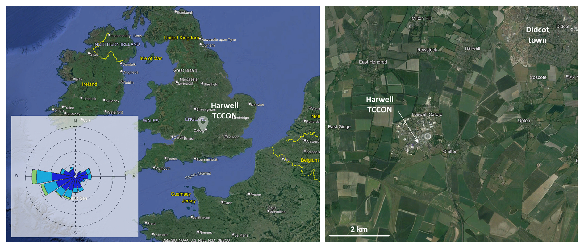
Figure 1 Harwell TCCON setting. Left, general site location within the UK. The insert in the bottom left gives the diurnal wind rose from the site wind measurements for September 2022 to September 2023. Dark blue, light blue, and green correspond to 1–3, 3–5, and 5–7 m s⁻¹ bins, respectively. The coordinate circles are spaced every 5 % frequency intervals. Right, close-up of the Harwell scientific campus indicating the mostly rural surroundings, apart for the small town of Didcot in the north-east. Background images © Google Earth.

The diurnal wind rose derived from the Harwell site meteorological station recorded between 14 September 2022 and 14 September 2023 is shown in an inset of Fig. 1. The retained data for the wind rose corresponds to the observational conditions: no rain, wind speed below 7 m s⁻¹, and at least 100 W m⁻² of solar flux. The prevailing winds are westerlies and south-westerlies. Considering the global air masses affecting the UK weather (UK Met Office, 2018), these correspond to the returning polar maritime and the tropical maritime air masses. The Harwell site is therefore well situated to obtain data on the large-scale atmospheric exchanges between the Atlantic and continental Europe. Local sources of greenhouse gases are primarily related to agricultural activities and some medium size urban centres. The closest town, Didcot, has a natural gas 1.4 GW power station that is a major local source of CO₂. However, the plant is located 6.5 km from the Harwell site on a bearing of 30°; the chance of transport to the Harwell site is less than 5 % according to the 2022 wind rose. Besides, the site is located upwind of London when considering the prevailing winds, which is of interest for the characterization of GHG emissions of the greater London area.

3 Instrumental system description

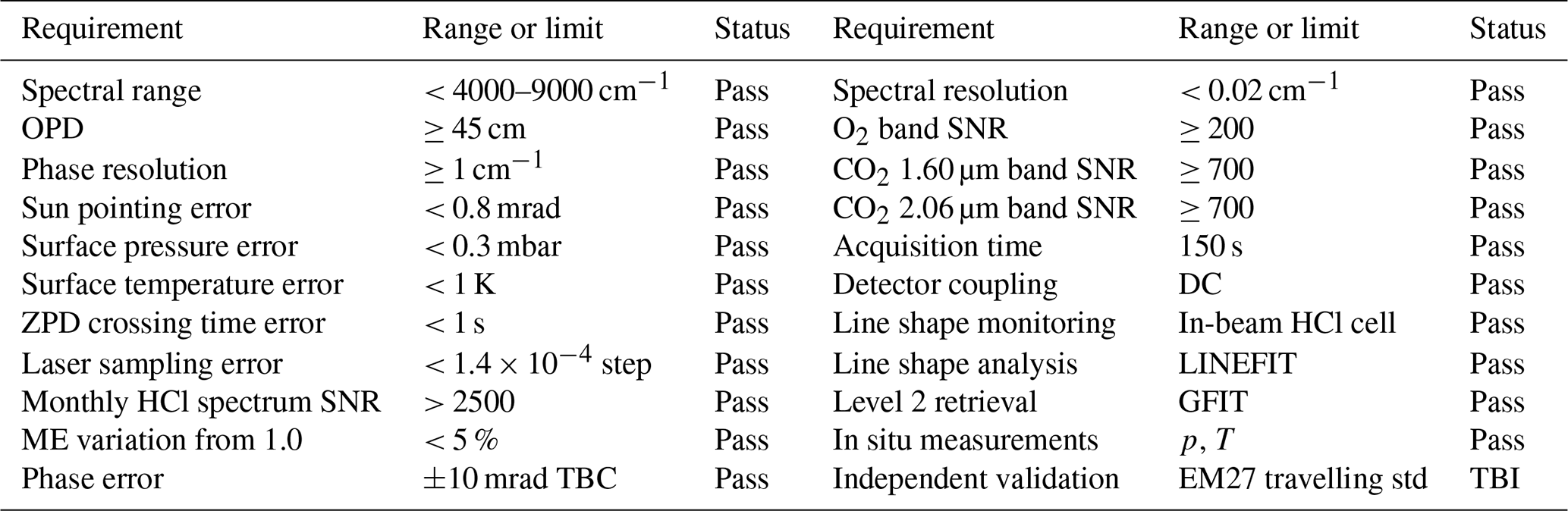
The description of the measurement system implemented at the Harwell site, as well as its verification described in the following sections, is underpinned and framed by the TCCON measurement system requirements (TCCON wiki, 2021). These are recalled in Table 1.

Table 1 Summary of the main instrumental requirements for a TCCON measurement system. The acronyms in the table stand for OPD: optical path difference; ZPD: zero path difference; HCl: hydrochloric acid (gas); SNR: signal-to-noise ratio; ME: modulation efficiency; TBC: to be confirmed; TBI: to be implemented.

3.1 Spectrometer

The spectrometer is a Bruker Fourier transform spectrometer (FTS) model IFS120/5 HR (S/N GI003092). The maximum optical path difference (OPD) is 6 m, leading to a maximum resolution of 0.0015 cm⁻¹ (per Bruker definition of resolution, which is $\mathrm{0.9}/\mathrm{OPD}$). A top view of the FTS with covers removed is shown in Fig. 2, in which an illustration of the optical path has been overlaid. At the bottom right is the source compartment. A flip mirror allows the radiation to be injected into the interferometer to be selected: either an internal source or external radiation entering on the side of the source compartment, so that it forms an image onto the input FTS aperture (field stop). The latter input is used for TCCON measurements. This input accepts an $f/\mathrm{6.5}$ beam (full angle of view of 8.7°) and enters with an angle of ∼ 7° to the normal to the input window.

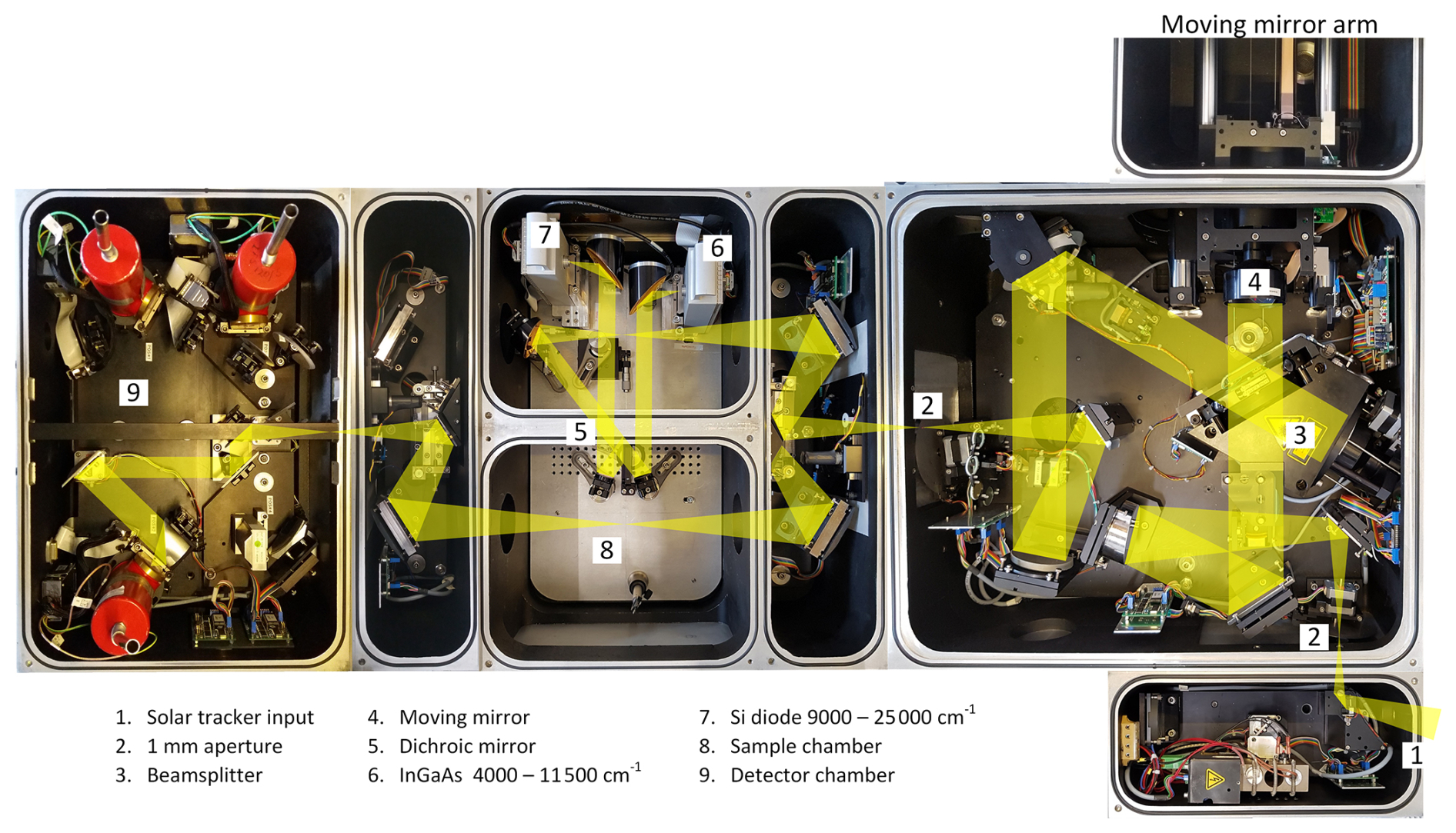
Figure 2 Top view of the opened Fourier transform spectrometer (FTS) with a representation of the optical path overlaid.

The exit aperture of the interferometer compartment is re-imaged at the centre of the sample compartment, in which the detectors have been installed. The beam is re-collimated and split into two components by a dichroic filter transmitting > 0.9 from 3700 to 11 200 cm⁻¹ and reflecting > 0.9 between 12 000 and 16 000 cm⁻¹. The high-frequency reflected part is focused onto a Si detector (area 1.2 mm²) by a 50.8 mm diameter and 50.8 mm focal length off-axis paraboloid (OAP) mirror. Before the focusing, an anti-aliasing filter (Thorlabs FGL665) is added into the beam (low-pass, 3 dB cut-off frequency of ∼ 15 900 cm⁻¹). Given the space constraint, the filter had to be inserted in the collimated part of the beam. It has been checked not to produce any significant fringing to the infrared and visible transmission spectra. The low-frequency part is transmitted to be focused in the same manner onto an InGaAs detector (area 1 mm²). In the figure, the detectors can be seen installed in the upper sample compartment. The optical arrangement has retained the option to use the other sample compartment (lower one in Fig. 2) together with a range of different detectors from the detector compartment.

The FTS is equipped with the dual acquisition electronics allowing for the simultaneous acquisition of the InGaAs and the Si detector signals. Outputs of the respective detectors pass successively through a pre-amplifier, a low-pass filter (LPF), and a main amplifier. For solar measurements, the detectors are operated in DC mode, unit gain is applied in all cases, and the cut-off frequency of the LPF is matched to the velocity of the scanning mirror. For HCl calibration spectra, using a tungsten lamp source, the detectors are operated in AC mode to increase the dynamic range and the InGaAs detector operated at an increased gain of 10.

The FTS is not operated under vacuum nor under inert atmosphere.

3.2 Sun tracking

A high-precision alt-azimuth solar tracker was built in-house based on the design of Robinson et al. (2020), with some adaptations described below, to capture the radiation input to be directed into the FTS. A rotation stage with a large central aperture of 120 mm diameter was used to control the pointing azimuth angle of the tracker. Its unidirectional angular repeatability is given to be 5 µrad (Physik Instrumente part no. PRS200 6449921111). The large aperture of the azimuth stage ensures that the distance between the tracker and the solar input coupling optics (517 mm effective focal length) can be as long as 12.9 m. The elevation angle of the tracker is controlled by another high-precision rotation stage with a 2 µrad repeatability (Physik Instrumente part no. L-611.9ASD). Azimuth and elevation plane mirrors are identical, made of 20 mm thick aluminium ellipses with dimensions of 184 mm × 130 mm. The mirrors are nickel and gold plated with a surface quality better than $\mathit{\lambda }/\mathrm{5}$ at 633 nm.

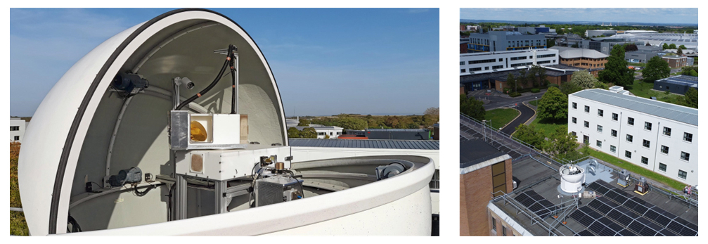
Figure 3 Left, view of the alt-azimuth high-pointing-precision solar tracker operating in the astronomical dome. Right, general view of the roof installation within the Harwell Campus (drone image courtesy of Melina Zempila).

To limit environmental exposure, the azimuth stage and the mirror assembly are housed in Delrin compartments, kept white to limit radiative heating. For structural strength, the elevation stage is enclosed in an aluminium compartment, protected by a pressed-steel radiation shield. The temperature of the stages is actively monitored: when the temperature exceeds 30 °C, a forced convection cooling is activated, and over 40 °C the system is switched off as being beyond the operational range of the stages to avoid damage. Resistive heating pads are activated when necessary to maintain the stage temperature above 10 °C. The whole system is installed in a motorized clam-shell dome (Baader Planetarium GmbH), installed on the roof of our laboratory within the Harwell Campus as shown in Fig. 3. The distance between the first mirror of the tracker and the input aperture of the FTS is 9.5 m.

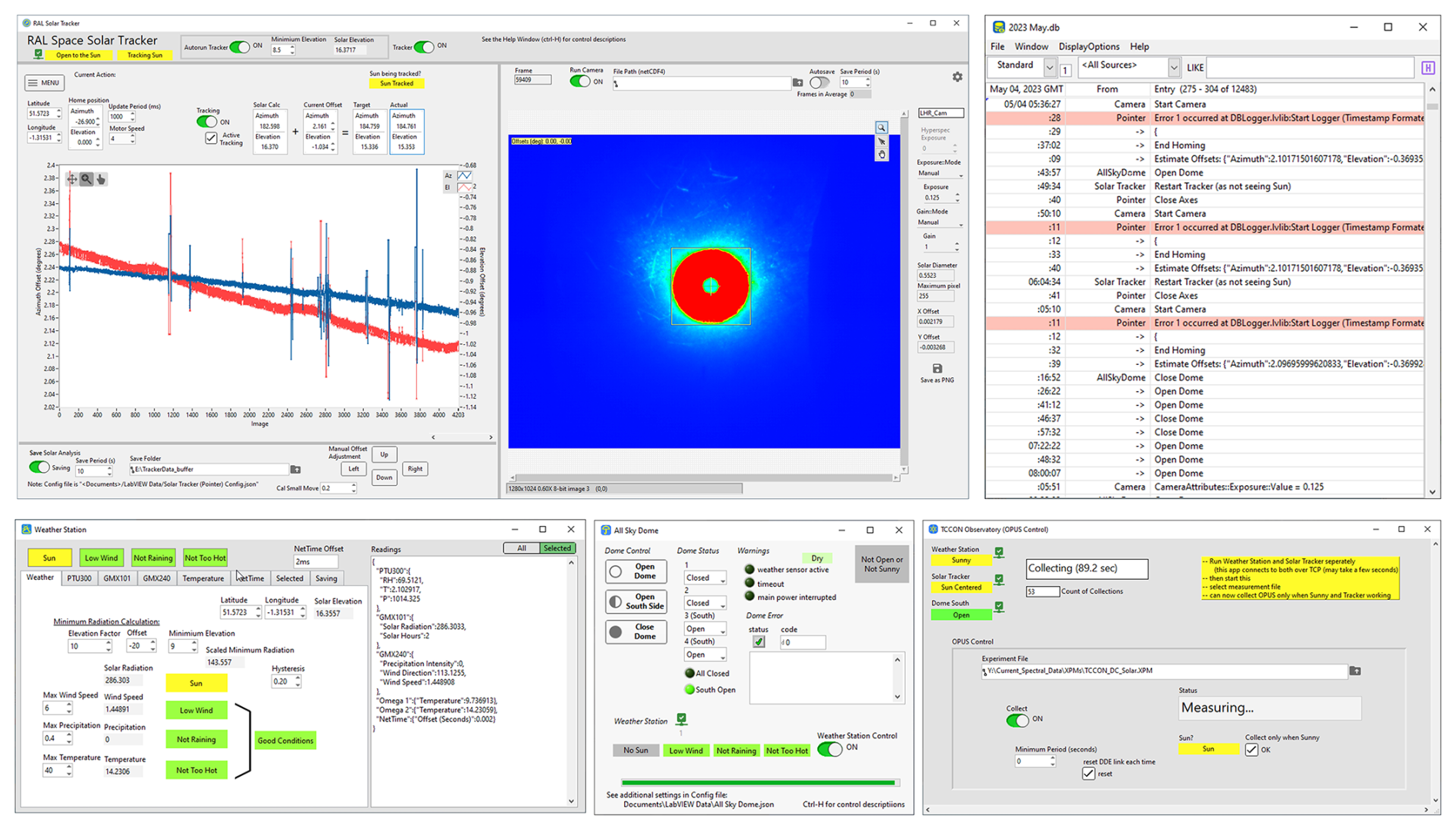
Figure 4 Composite picture of the graphical user interfaces of the five independent LabVIEW applications underpinning the Harwell site automated operation. Clockwise from top left, solar pointing, camera control, log database of operation events, OPUS FTS control interface, dome operation, and weather station control. The camera image shows the video of the FTS input aperture plane. In the figure the saturated image of the sun disc co-aligned to the 1 mm input aperture can be seen.

Together with the sun pointing hardware, a dedicated feedback system was developed using the camera tracking approach (Gisi et al., 2011) and programmed with LabVIEW. An HD CMOS camera (1280 × 1024) equipped with a 20 mm focal length bi-convex lens is inserted into the source compartment of the FTS to produce an image of the interferometer input aperture plane with a magnification of 0.25. Because of the volume taken by the switching mirror assembly for input selection within the spectrometer, the camera system could only be inserted at a 15° angle with respect to the normal of the input aperture plane. The camera is aligned so that its central pixel corresponds to the centre of the FTS input aperture image. A picture from the feedback camera in false colour taken by the CMOS camera during operation is shown in the central part of Fig. 4.

Within the LabVIEW control software, once all the conditions are fulfilled to start direct solar measurements, the tracker points to the theoretical apparent location of the sun given the time and the geolocation. The SUNAE algorithm is used for the calculations (Walraven, 1978; Michalsky, 1988), implemented in LabVIEW. Due to the imperfect alignment of the tracker, the solar disc may not be within the 2.2° × 2.8° field of view of the tracking camera when the system goes on. In this case, a database of offset corrections generated from historical data is used. Once the sun is within the image, the National Instruments Vision library is used to recognize the vector between the position of the solar disc centre and that of the FTS central aperture. Motion correction signals to the alt-azimuth stages are then sent for re-centring. The pointing update rate is 1 Hz. The transfer function between the alt-azimuth angles and the camera image reference frame axis requires a three-point sensitivity calibration. This is measured by purposely generating a known change in azimuth and elevation angles while the sun is centred and determining the corresponding pixel vector change observed for the sun's centre in the camera image. Sensitivity and offset calibration needs repeating only if the optical alignment of the solar radiation delivery arm is altered.

3.3 Calibration cell input

By default the spectrometer input is the solar scene. By manually changing a plane and an OAP mirror using pre-aligned magnetic posts, it can be switched to the calibration cell input. The cell is filled with pure HCl at 4.865 hPa pressure (Hase et al., 2013). For the calibration arm, the light source is a tungsten halogen bulb (Osram, 50 W, 12 V, 900 lumen) collimated with a 25 mm diameter, 40 mm focal length calcium fluoride (CaF₂) lens. A spherical confocal reflector behind the lamp also collects some radiation. The collimated light is directed through the HCl calibration cell (100 mm long, 25 mm diameter, ∼ 5 mbar pressure) and then focused into the spectrometer using an OAP ($f/\mathrm{7}$, focal length 17.8 cm) to form an image on the FTS input aperture wheel. The calibration cell currently used for this external calibration, carried out monthly, was provided by the TCCON community and calibrated with the parameters listed in Table 2, cell ID 49. Residual cell impurities such as air and water vapour require the use of effective cell parameters for network-wide consistency of line shape monitoring to avoid the need to provide separate partial pressures for all constituents. The effective pressure is the pressure of pure HCl that would give the observed linewidths in the presence of impurities (Hase et al., 2013).

Table 2 Description of the two calibration HCl gas cells used for Harwell site calibration.

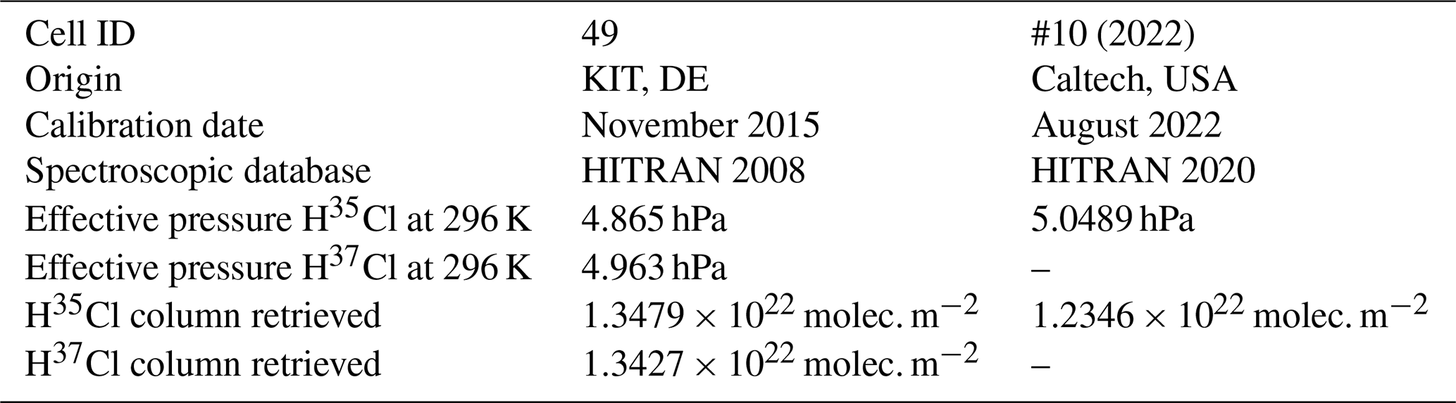
In June 2021, in accordance with a change in TCCON protocol, the HCl calibration cell was placed in the solar beam when not in use for the periodic external calibration to provide an additional quality metric output from the data processor described in Sect. 5. A duplicate cell was therefore acquired for redundancy, whose properties are also given in Table 2.

3.4 Meteorological station

The meteorological station is composed of (1) an anemometer and a rain gauge (Gill Instruments Maximet GMX240); (2) a sun pyranometer (Gill Instruments Maximet GMX101); and (3) a pressure (p), temperature (T), and relative humidity (RH) sensor (Vaisala PTU-307). The p, T, and RH sensor is calibrated every year to maintain accuracies of ±0.20 hPa at 20 °C, ±0.2° at 20 °C, and ±1 % for a 0 %–90 % RH range. A duplicate p, T, and RH sensor system, re-calibrated by the manufacturer and swapped annually, allows continuous logging of data to TCCON accuracy standards.

All meteorological data are time-stamped, acquired with a 1 Hz rate, smoothed, and logged every minute using the TCCON observatory LabVIEW control software.

3.5 Timing

To ensure accurate time-stamping of the acquired spectra, the TimeTools T100 Network Time Protocol server was used to synchronize the control PC of the FTS with an accuracy of 3 ms. The spectra acquired receive their timestamp from the internal FTS controller, which, via the OPUS software, is synchronized from the control PC of the FTS running OPUS (Kivi and Heikkinen, 2016; Pauli Heikkinen and Rigel Kivi​​​​​​​, personal communication, 2020). On the control PC, the Bruker OPUS software was set to update its time reference from the PC clock every hour. The GPS antenna connected to the TimeTools server was installed on the pole holding the meteorological instruments referred to above.

The timestamps of the spectra as contained in the OPUS format files are then used to calculate the zero path difference (ZPD) timestamp as described in Toon (2009). Early on, an anomaly was found in the way interferogram peak locations are stored in the data output from the OPUS software, specifically associated with the FTS firmware version 2.485. The solution was implemented as part of the processing chain and is described in Sect. 5.

3.6 Observation automation

To benefit from the increased data throughput brought by observation automation (Geddes et al., 2018; Geibel et al., 2010), purpose-built LabVIEW software was developed. It controls all the subsystems required for conducting measurements (dome, sun tracker, meteorological station, spectrometer) as well as the overall measurement schedule and its automation.

The automation software is divided into a set of independent applications that communicate with each other over TCP connections. They can even be distributed across separate computers. Figure 4 shows the graphical user interface of some of the applications.

The “weather station” application collects data from the meteorological measurement hardware and also the temperature from the sun tracker rotation stages. From the data collected, it determines whether the dome needs opening or closing. The following conditions are required to trigger dome opening:

• Sun elevation must be above 10°.

• Sun flux must be above a previously recorded threshold during clear-sky conditions, given the solar elevation angle.

• Precipitation must be < 0.08 mm h⁻¹ (the sensor resolution).

• Wind velocity must be below 6 m s⁻¹.

The “all sky dome” application controls dome operations, based on inputs from the “weather station” one or from manual operation if the “weather station” application is not running. To avoid short sunny spells, frequent in the south-east of England, activating frequent opening/closing sequences, the opening conditions must be fulfilled for at least 5 min to trigger the actual opening. Similarly, the dome closes if any of the observation conditions is not fulfilled for a continuous period of 5 min. If rain is detected by a sensor integrated into the dome by the manufacturer, however, closure is immediate.

The “RAL tracker” application controls the sun tracker hardware and the associated camera and calculates the tracking feedback. It communicates with the “all sky dome” application, as sun tracking is obviously dependent on the dome status, and with the “FTS control” application that needs to know if spectra acquisition is required.

The “FTS control” application communicates with the “RAL tracker” one and with the OPUS software installed on the FTS control computer. OPUS does not support TCP communication and imposes instead the fairly old DDE (dynamic data exchange) communication standard.

All the applications mentioned communicate with the “log viewer” one, which provides a user interface to look at log files and events created by the individual applications organized as a searchable database.

During operation, all the files (OPUS files, meteorological data file, automation log files) are written locally on the FTS control PC. The Task Scheduler of the Windows OS was used to automate the daily transfer of the local files to a backed-up archive. Every day at 23:55 LT, the files of the day are transferred, ready for processing.

4 System performance

The performance of the instrumental system is evaluated against the requirements set by the TCCON community (Wunch et al., 2011a) summarized in Table 1. Some requirements relate to the settings of the FTS and are not detailed any further. In this section the focus is on the instrument performance characterization.

4.1 Signal-to-noise ratio

When measuring transmission spectra of the atmosphere, the signal-to-noise ratio (SNR) achieved for the short wave infrared region (InGaAs detector channel) is maintained between 300 and 600, depending on atmospheric conditions and elevation angles. The input optical signal is attenuated to avoid detector saturation that may trigger interferogram non-linearity. Some examples of estimates, from the residuals of the transmittance spectral fittings, can be seen in Sect. 5. From these particular residuals, the SNR is 463 (417) for the CO₂ window centred at 6340 cm⁻¹ (CH₄ window centred at 6002 cm⁻¹). The sun elevation was 27°, about half of the maximum one achievable at the Harwell location in the summer. The infrared region (Si detector channel) provides SNR of about 250 for the measurement of the O₂ A-band (760 nm, 13 000 cm⁻¹).

The expected SNR from the instrument can be estimated using, for instance, the simplified expression from Treffers (1977) for a rapid scanning interferometer. In the case of TCCON direct solar measurements, which use a bright source, we consider the photon shot noise as dominating. The corresponding noise equivalent power (NEP) for purely Poissonian unpolarized light is expressed by Eq. (1), with P_ν the spectral flux detected by the detector (includes quantum efficiency). Calculating the expected SNR, given the InGaAs and Si detector spectral responses, gives 700 and 900, respectively. This is within the order of magnitude of what is observed, given the simplicity of the SNR model.

$$\begin{array}{}\text{(1)}& {\mathrm{NEP}}_{\mathrm{ph}}^{\mathrm{2}}=\mathrm{2}\int h\mathit{\nu }{P}_{\mathit{\nu }}\mathrm{d}\mathit{\nu }\end{array}$$

When the calibration measurements are made with the external source, 200 repetitions of the standard single-sided forward–backward acquisition are averaged to produce a spectrum with an SNR of 3000. The acquisition time is approximately 8 h.

4.2 Instrument calibration

The instrument performance is monitored each month by measuring and analysing a high-SNR transmission spectrum of the HCl calibration cell (ID: 49), as described in Hase et al. (1999). The LINEFIT analysis software is used to infer the instrument line shape (ILS) from the experimental HCl spectral lines, as any line shape uncertainty will contribute to error in the retrieved gas DMF (Hase et al., 2013).

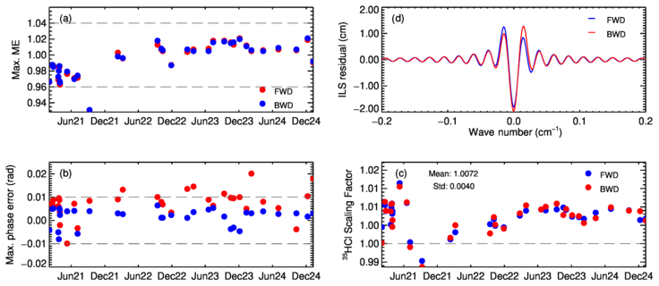
Figure 5 Extrema of the ME (a) and phase error (b) observed in each ILS measurement made over the last > 3 years of operation. (c) Corresponding H³⁵Cl column normalized to the independently calibrated value. (d) Example of residual between the ILS determined by LINEFIT and the theoretical ILS used in the retrieval processing software.

The simple parametrization of the ILS model was used when running LINEFIT. The spectral window of analysis was selected to be 5670–5805 cm⁻¹. The results of more than 3 years of monthly ILS measurements are summarized in Fig. 5. The variation in spectrometer modulation efficiency (ME) is consistently well within the requirement 0.95 < ME < 1.05 over the full range of OPDs, as seen in Fig. 5 which shows the extreme values of ME picked up from each of the ME vs. OPD output analyses. The repeated column value for H³⁵Cl shows a systematic bias of 0.7 % and a 1σ scatter of 0.4 %. The residual between the LINEFIT-inferred ILS and the modelled one used in the retrieval processor shows small discrepancies. In the near future, we will look into using the measured line shape as the input parameter for column retrieval.

4.3 Sun pointing

The RAL sun tracker precision was assessed using the record of the actual azimuth and elevation angles as reported during a tracking event. To extract the short-term random error element, azimuth and elevation records are subtracted from the calculated theoretical sun pointing. The residual offsets (differences between actual and calculated angular positions) are further de-trended from slowly varying biases using a polynomial fit over a 1 h duration before evaluation of the standard deviation. Figure 6 shows an example of data from 25 May 2023, when an (almost) full day of clear sky was available. Over a 2 h period, the pointing precision is 56 and 17 µrad for azimuth and elevation angles, respectively.

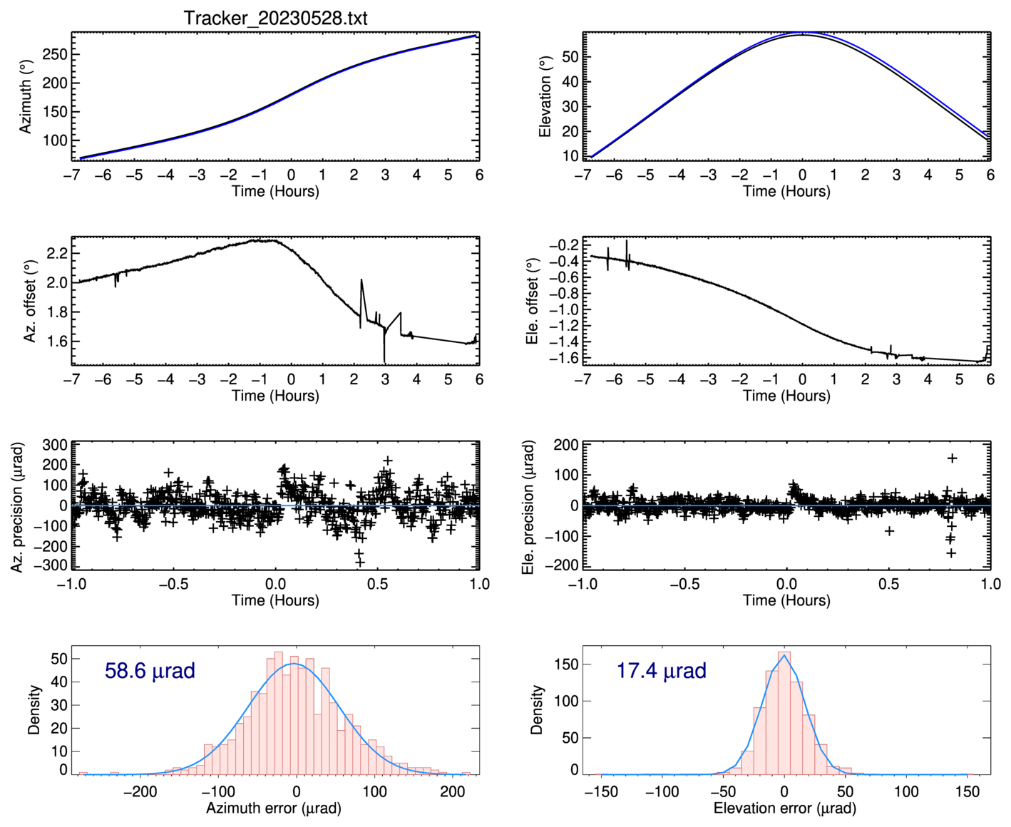
Figure 6 Estimation of the sun tracker precision. The first (second) column corresponds to the azimuth (elevation) coordinate. From top to bottom, the plots represent (1) the actual and calculated angular coordinates of the sun centre, (2) the residuals between actual and calculated angular coordinates, (3) the residuals further de-trended by a polynomial over a 2 h period, and (4) the histograms of the above with a fitted Gaussian distribution whose standard deviation is given in the plot.

The presence of common absorbing species in both solar and Earth atmospheres allows an estimate of the accuracy to be made by observing the Doppler shift in the solar absorption line compared to the terrestrial. We follow the simple “single angle” approach described by Gisi et al. (2011) and Robinson et al. (2020) to estimate the pointing accuracy rather than the full dual-axis estimation reported by Reichert et al. (2015). The relationship between θ, the angle subtended between the sun centre and any point along the sun equatorial axis for an Earth observer, and the apparent solar line frequency ν is expressed by Eq. (2), in which R_s is the sun radius, d the Earth–sun distance, v_T the equatorial tangential velocity of the heliosphere, ν₀ the terrestrial line frequency, and c the speed of light. The term in the arcsin function is always smaller than 1 ‰ in all practical cases; therefore we can approximate arcsin (x)=x, which leads to the expression of the pointing angular deviation θ as a linear function of the relative Doppler shift $\mathrm{\Delta }\mathit{\nu }/{\mathit{\nu }}_{\mathrm{0}}$.

$$\begin{array}{}\text{(2)}& \mathit{\theta }=\arcsin \left[{\displaystyle \frac{c\cdot R_{\mathrm{s}}}{v_{\mathrm{T}}\cdot d}}\cdot \left({\displaystyle \frac{\mathit{\nu }}{{\mathit{\nu }}_{\mathrm{0}}}}-\mathrm{1}\right)\right]\approx {\displaystyle \frac{c\cdot R_{\mathrm{s}}}{v_{\mathrm{T}}\cdot d}}\cdot {\displaystyle \frac{\mathrm{\Delta }\mathit{\nu }}{{\mathit{\nu }}_{\mathrm{0}}}}\end{array}$$

As part of the processing (to be described in the next section), the relative Doppler shift observed in the recorded spectra is determined from spectral fitting and can then be used as an estimator of pointing accuracy using Eq. (2). Figure 7 shows the estimated pointing accuracy as derived from Doppler shift for nearly 4 years (2020–2024).

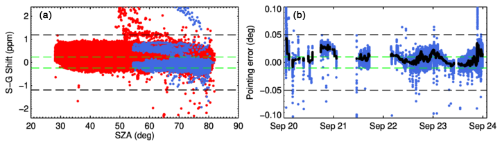
Figure 7 Estimation of the sun tracker accuracy from solar line Doppler shift. (a) Solar gas shift (ppm) and pointing error (deg) vs. solar zenith angle (SZA). Blue is AM measurements, red is PM measurements, the black dash is ±0.05° limit for max accepted error, and the green dash is ±0.01 (ideal TCCON) limit for pointing error. (b) Pointing error time series for 4 years (September 2020 to September 2024). Blue signifies pointing error, black is the rolling median of the spectra, and dashed lines are as previously.

4.4 Non-linearity

The model used to process the data assumes linearity of the optical detectors. Any non-linearity between the photon flux received by the photodetectors of the FTS and the corresponding recorded signal can be identified by a distortion of the low-pass-filtered interferogram in the vicinity of the zero path difference (Abrams et al., 1994). This distortion exhibits a peak-like structure (Keppel-Aleks et al., 2007), from which a non-linearity metric is derived: the so-called “dip” expressed as the amplitude of the distortion peak relative to the unmodulated interferogram amplitude. The non-linear distortion of the detector output relative to the photon flux can be due to either detector saturation, resulting in a negative dip, or an artefactual supra-linearity, resulting in a positive dip (Corredera et al., 2003).

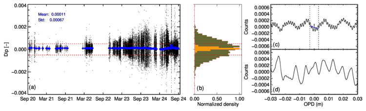
Figure 8 (a) Evolution of the dip metric outputted by GGG over the whole Harwell site dataset. The blue points are a 1000 point smoothing, the red lines indicate the required norm to ensure insignificance of non-linearity to the retrieved products. (b) Corresponding histogram of two data subsets. The dark (light) histogram corresponds to January to April 2024 (March to June 2021). The right-hand-side panel shows smoothed, DC-corrected interferograms. (c) From 1 June 2021, the vertical lines indicate the ZPD area where the peak is searched and the blue line the baseline correction for its normalization. (d) The same but from 21 March 2024. Both interferograms exhibit electrical noise pickup at mains frequency and harmonics.

The dip metric, as derived by the processor, for the Harwell site is shown in Fig. 8. Considering the global mean of the dataset, the instrument appears to be affected by a slight non-linearity (supra-linearity). However, individual estimates of dip are often outside the network norm (±0.5 ‰), with a large scatter that increases significantly with time, whilst the probability distribution function remains Gaussian. The histogram plots in Fig. 8 are for two subsets of 100 d each, starting respectively from 21 March 2021 (clear histogram) and from 1 January 2024, and illustrate the widening of the scatter. The random nature of the dip metrics raises doubts as to whether it originates from true non-linearity in this case.

To investigate further in an independent manner, the “out-of-band” regions of the InGaAs spectrum where no signal is expected were scrutinized. With detector non-linearity, the self-convolution of the spectrum produces a quadratic spectral artefact in the out-of-band regions between 0 and > 4000 cm⁻¹ (Kleinert, 2006). Spectra were selected from dates between June 2021 and June 2024, taking in each case a spectrum from early morning, noon, and late evening. Looking at the 3800–3900 cm⁻¹ region for these spectra, no statistically significant offset was measured, indicating no non-linearity.

The dip parameter ought to be related to the power reaching the detector and to increase as the detector becomes more heavily saturated. By taking the unmodulated level of the interferograms as a proxy for optical power, no correlation with the dip amplitude was observed for either detector channel.

Significant interference (at 50 Hz and harmonics) can be seen in our interferograms. The source was confirmed as being electrical in nature by varying the scanning velocity of the moving mirror of the interferometer. Using a tool developed by the Bremen site team (Buschmann, 2024), the actual dip, if any, can be visualized. Two cases are shown in the right-hand-side panel of Fig. 8c and d. Figure 8c shows a smoothed, DC-corrected interferogram from 1 June 2021 at 14:51 UTC. The vertical lines indicate the region around the ZPD in which the dip amplitude is determined and normalized to the unmodulated interferogram amplitude (blue line) to generate the dip parameter. The value for the case illustrated is 0.11 ‰. Figure 8d shows a similar trace for an interferogram from 21 March 2024 at 13:02 UTC. This suggests that the dip parameter is largely determined by the instantaneous properties of the electrical interference and so is not a reliable indicator of non-linear detector behaviour. We are currently working to identify the source of the interference.

4.5 Laser sampling error

The spectrometer is fitted with the laser sampling board (LSB) developed for the TCCON. It allows the optimization of the DC offset to the HeNe laser signal that provides the optical frequency reference to reduce the asymmetry in sampling interval and hence reduces ghosting. Using a narrow-band filter at 6060 cm⁻¹ to test the suppression, the ghost $/$ parent suppression ratio was measured to be $\approx \mathrm{5}\times {\mathrm{10}}^{-\mathrm{5}}$. The laser sampling errors as outputted by the I2S software converting interferograms to spectra are Gaussian distributed with a mean of $-\mathrm{5}\times {\mathrm{10}}^{-\mathrm{6}}$ and a standard deviation of $\mathrm{1.1}\times {\mathrm{10}}^{-\mathrm{4}}$, expressed as the fraction of sample step. This is well within the requirement of less than $\mathrm{2.4}\times {\mathrm{10}}^{-\mathrm{4}}$.

5 Data processing

5.1 Processing chain

The data processing chain has been implemented using the latest version (2020) of the GGG software (Laughner et al., 2024; Wunch et al., 2025). The level 1 data are time-stamped transmission spectra of the atmosphere produced from the FTS interferograms and associated metadata. The I2S software (2020 release) performs the fast Fourier transform of single-sided interferograms into spectra, including the removal of low-frequency intensity fluctuations and Mertz phase correction. A script checks and only keeps the measurements where both channels are present and prepares the corresponding list for ingestion into GGG.

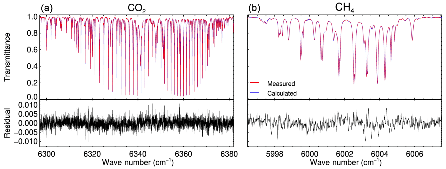
Figure 9 Examples of spectral fit and residual outcomes. (a) CO₂ micro-window centred at 6339 cm⁻¹ from 17 July 2023 at 08:25 UTC. (b) CH₄ micro-window centred at 6002 cm⁻¹ from the same record.

Within the GGG software, a non-linear least-squared fitting of the level 1 data with an atmospheric transmission model is iteratively performed by scaling an a priori vertical profile of volume mixing ratios (VMRs) of atmospheric gases until convergence between calculated and measured spectra is achieved and the residual is minimal, as seen in Fig. 9. The profiles are only scaled, so the vertical distribution of the a priori profile is preserved. The output of this fitting consists of total column abundances V_Gas of each gas in molecules per square centimetre being the vertical integral over each profile. The a priori gas VMR, pressure, and temperature profiles originate from the near-real-time GEOS meteorological dataset referred to as FP-IT (Forward Processing for Instrument Team), switched to GEOS-IT on 1 April 2024. For the TCCON, Caltech produces the extrapolated dataset relevant to each site, made available with a timeliness of 24 to 48 h (Laughner et al., 2023).

The processor then uses correction factors for each retrieved species: one to account for mostly spectroscopy errors producing a bias on column abundances dependent on the solar zenith angle (air-mass-dependent correction factor – ADCF) (Wunch et al., 2011a) and one which is a global scaling (air-mass-independent scaling factor – AICF) designed to anchor the retrieved X_Gas product to World Meteorological Organization (WMO)-traceable in situ measurements (Wunch et al., 2010). Currently, in the absence of an independent site scale-factor determination, the Harwell site processor uses the values that have been updated for the GGG2020 software release and are given in Laughner et al. (2024). We are planning to attempt a site-specific update to the correction factors (Pollard et al., 2021) using the travelling standard methodology (Herkommer et al., 2024). The level 2 output data produced are column-averaged DMFs of gases, X_Gas, defined by Eq. (3), where $f_{{\mathrm{O}}_{\mathrm{2}}}$ is the known mean DMF of O₂ in the well-mixed atmosphere. The calculation of X_Gas by reference to the column abundance of O₂ reduces the sensitivity to errors in sun pointing and surface pressure measurements, among other advantages, as outlined in Wunch et al. (2011b) and Laughner et al. (2024).

$$\begin{array}{}\text{(3)}& X_{\mathrm{Gas}}={\displaystyle \frac{V_{\mathrm{Gas}}}{V_{{\mathrm{O}}_{\mathrm{2}}}}}\cdot f_{{\mathrm{O}}_{\mathrm{2}}}\end{array}$$

A diagnostic quantity, X_Luft, is also calculated. It represents the ratio of two distinct means of calculating the air DMF: one from surface pressure and the other from the O₂ column retrieval (Laughner et al., 2024). X_Luft should ideally be unity, with deviations of even a few per mil being indicative of retrieval bias.

After the production of the level 2 data by GGG, the dataset is submitted (typically every quarter) for independent data quality assurance and control (QA/QC) by the network. Over the year 2023, for example, about 62 % of the data submitted passed the QA/QC. The primary reason for flagging a measurement as being of insufficient quality is cloud contamination.

Whilst using the standard GGG2020 retrieval, Harwell site-specific “pre-processing” tasks have been implemented and are briefly described below.

5.1.1 Timing inconsistency correction

During early data analysis, a systematic significant forward–backward scan bias in the X_Luft reported was observed (Brownsword et al., 2021). An inconsistency in the way the interferogram peak locations for forward and backward scans are stored in the OPUS files for the two detector channels was found. It was confirmed that it arises from version 2.485 of the Bruker IFS125 firmware (David Pollard, personal communication, 2021), also observed at the Lauder TCCON site (Pollard et al., 2017).

With this particular firmware, the parameter storing the peak location of the forward scan for the second (InGaAs) detector introduces an incorrect value to I2S and produces a > 10 s timestamp error. We followed the solution implemented by the Lauder team, and a Python routine reconstructing the OPUS file with the corrected interferogram peak locations was integrated into the processing chain. As more TCCON facilities encountered the same issue, the TCCON partners agreed on a unified approach for the correction to be part of the main algorithm to be implemented in the next GGG2020 version (Griffith and Laughner, 2024).

5.1.2 In situ meteorological data ingestion

Meteorological parameters are recorded independently of the TCCON measurements as described in Sect. 3.4 but on a synchronized timescale. Before starting the GGG processing, time series of temperature, pressure, and relative humidity are extracted and assigned to each forward–backward interferogram measurement. The zero path difference (ZPD) times of the forward and backward interferograms are calculated, and the meteorological data are interpolated with a spline fit at the central time between the two ZPD times, i.e. approximately 75 s after the forward interferogram ZPD. The two ZPD times differ by about 150 s, the time it takes to record the two interferograms.

5.2 Dataset

The Harwell dataset covers about 4 years of operation at the time of writing (Weidmann et al., 2023). The record was started with a site manually operated during business hours, therefore limited in terms of data throughput. Between December 2021 and February 2022, the site was relocated to a different laboratory a few tens of metres away and did not operate. Between June 2022 and November 2022, a significant failure of the controller of the rotation stages, part of the sun tracker, and subsequent long delivery time for repairs prevented any measurements from taking place. From November 2022 onwards, system automation started to be deployed and a significant increase in data throughput is noticeable.

Figure 10 shows the $X_{{\mathrm{CO}}_{\mathrm{2}}}$ temporal series, together with a fit of the seasonal variation model developed by Lindqvist et al. (2015) and given in Eq. (4), where t is the time in days and $\mathit{\omega }=\mathrm{2}\mathit{\pi }/T$, where T = 365 d.

$$\begin{array}{}\text{(4)}& \begin{array}{rl}{X}_{{\mathrm{CO}}_{\mathrm{2}}}\left(t\right)& =a_{\mathrm{0}}+a_{\mathrm{1}}t+a_{\mathrm{2}}\sin \left(\mathit{\omega }\right[t-a_{\mathrm{3}}]\\ & +{\cos }^{-\mathrm{1}}\left(a_{\mathrm{4}}\cos \left(\mathit{\omega }[t-a_{\mathrm{5}}]\right)\right))\end{array}\end{array}$$

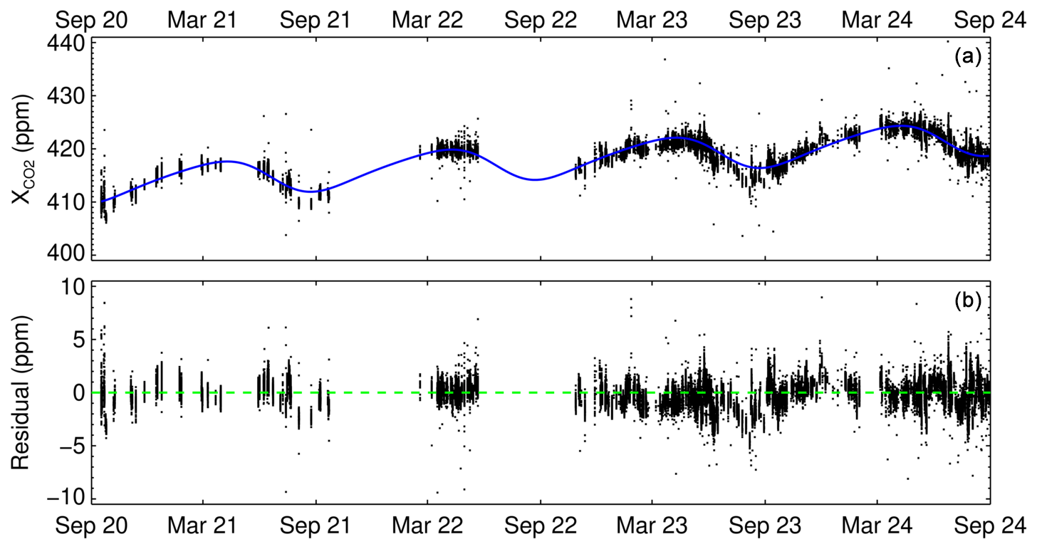
Figure 10 Harwell site $X_{{\mathrm{CO}}_{\mathrm{2}}}$ dataset (black dots). The temporal geophysical cycle was fitted to the model proposed by Lindqvist et al. (2015), shown as a blue line. Panel (b) provides the residual between the measured $X_{{\mathrm{CO}}_{\mathrm{2}}}$ and the modelled one.

The bottom panel of Fig. 10 shows the residual between the data and the model. The model was fitted to the data using a Levenberg–Marquardt least-squares algorithm. The uncertainties on $X_{{\mathrm{CO}}_{\mathrm{2}}}$ derived from the GGG retrieval were fed into the fitting routine to propagate down to the seasonal cycle model parameters. The reduced χ² after fit convergence was 2.8, indicating a good input error scaling. The resulting model parameters and their uncertainties are given in Table 3.

Table 3 Fitted parameters of the Lindqvist model describing the Harwell $X_{{\mathrm{CO}}_{\mathrm{2}}}$ seasonal cycle.

The linear increase in $X_{{\mathrm{CO}}_{\mathrm{2}}}$ with time (coefficient a₁ in Table 3) is described by a gradient of 2.11 ppm yr⁻¹. This is slightly less than the global 2.49 ppm yr⁻¹ rise averaged over 2021–2023 (Lan et al., 2024). The averaged seasonal cycle amplitude over the dataset ($\mathrm{2}\left|a_{\mathrm{2}}\right|$ from Table 3) is 6.48 ppm. For comparison to not-so-distant measurements at a similar latitude, the amplitude appears lower than a typical temperate continental European TCCON site such as Bremen (53.1° N, 8.85° E), reported as 7.9 ppm (Jacobs et al., 2021), and higher than the 5.6 ppm (2000–2028 average) reported from in situ measurements from Mace Head (53.3° N, 9.9° W) (Yun et al., 2022; Schuldt et al., 2023). The residual plot in Fig. 10 also shows that seasonal cycle amplitude is not constant over the 4 years of record. The mid-September 2023 trough is underestimated by the model. Lastly, the seasonal cycle phasing can be described by the half drawdown day, which is day 169 from the fitted model, well within the fairly scattered reported ensemble (Jacobs et al., 2021).

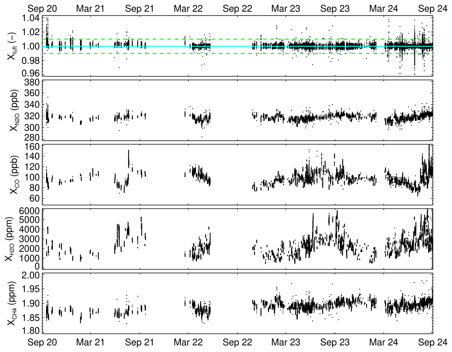
Figure 11 Harwell site column-averaged DMF for the main molecules measured by the TCCON system.

An excerpt of some other gas column DMFs obtained from the Harwell site is shown in Fig. 11. The plot also shows (upper panel) the column-averaged amount of dry air “X_Luft”, which ideally should be equal to 1, and therefore can be used as a data quality diagnostic as described earlier. The horizontal lines visualize the ±1 % deviation from the ideal case. The vast majority of the data are well within the required interval.

For $X_{{\mathrm{CH}}_{\mathrm{4}}}$, the annual trend is not constant: the annual rise over the years 2021 and 2023 is, respectively, 18.97 ± 0.20 and 9.86 ± 0.08 ppb yr⁻¹, well within the global trends of 17.91 and 9.88 observed (Lan et al., 2024). The year 2022 was not calculated because only 3 months of data is available for 2022.

Within the dataset, some events are noticeable. In spring–summer 2023 plumes from the Canadian wildfires travelled over to Europe. For distinct days in May and June 2023, the CO total column at Harwell increased by over 20 ppb compared to background days, producing spikes in the X_CO time series in Fig. 11. These events were corroborated using the near-real-time visualization tool from the Remote Sensing Group from RAL space (Latter et al., 2024), showing data derived from MetOp-B and MetOp-C with the Infrared Microwave Sounding retrieval scheme (Pope et al., 2021). Another similar event was observed again from the Canadian fires in August 2024.

6 Conclusions

The consistency and the data quality required across the global TCCON are essential to ensure the network fulfils its demanding purposes of (i) greenhouse gas satellite data validation, (ii) linkage between in situ and space-borne greenhouse gas measurements, and ultimately (iii) contributing to improving our knowledge of the carbon cycle. In this work, we transparently reported on the development and characterization of a new partnering observatory to demonstrate traceability of the Harwell site dataset quality down to the measurement system and provide reference information about it.

The establishment of the Harwell TCCON observatory and its automation has been thoroughly described and its performance characterized against the requirements agreed by the network, from instrumental parameters to data product quality metrics. The in-house solar tracker system developed for the observatory was found to maintain the pointing accuracy very well. The particular firmware of the Fourier transform spectrometer used was found to suffer from a timing zero-path difference inconsistency. This has been corrected within the processing flow. Despite being free of non-linearity, the non-linearity “dip” indicator was found to be affected by low-frequency electrical pick-up noise (< 150 Hz) producing artefactual non-linearity flagging.

The observatory has now produced a dataset spanning 4 years for averaged-column DMFs of CO₂, CH₄, CO, N₂O, H₂O, HDO, and HF, which have been confirmed to be of the required quality through the TCCON independent quality control process. The CO₂ seasonal cycle was characterized to be consistent with expectations for a northern mid-latitude location. CO spikes originating from plume transport from the Canadian forest fires were observed in both summer 2023 and 2024.

In the near term we are planning to further improve the site by (1) installing a permanent alignment monitoring tool for the interferometer, (2) verifying the Harwell site consistency with some of the TCCON partners through the travelling standard methodology, and (3) improving on the data timeliness of the system.