Optimal site selection for Choutuppal geomagnetic observatory, based on geophysical evidence

The phases of development of Choutuppal magnetic observatory over the last 15 years have enabled the effects of the natural environment like groundwater changes and lightning activity on the magnetic data to be evaluated. A high-resolution survey of total field anomalies led to the construction of a 2D model of the shallow surface. Constrained by conductivity depth slices from previous electrical resistivity tomography and electrical vertical resistivity imaging surveys, the distribution of sandy regolith, saprolite and granitic layers in the shallow subsurface is delineated. The pattern of lightning strikes in a 10 km area around the observatory is correlated to modulations and disruptions in the magnetic data. The analysis as a whole provides information for selecting a location to install a secondary variometer room by taking into account topography, lightning effect, soil resistivity, low magnetic anomaly and distance from the recharge pond, which can produce continuous data of higher quality and consistency than at present.

1 Introduction

Choutuppal (CPL) geo-electric observatory (geographic coordinates: 78.920° E, 17.290° N; geomagnetic coordinates: 149.24° E, 7.47° N) of CSIR-NGRI was established near the town of Choutuppal in the Yadadri Bhuvanagiri district, approximately 60 km southeast of the city of Hyderabad, in the state of Telangana (Sanker Narayan, 1964). The region primarily comprises granite and gneissic formations. These rocks are part of the Peninsular Gneissic Complex, which is one of the oldest geological formations in India, dating back to the Archean era. The weathering of the granitic and gneissic rocks has led to the formation of red and lateritic soils. The granitic formation is encroached locally by discontinuities such as dikes or quartz reefs, but these are not present on the site (Guihéneuf et al., 2014). The area around CPL observatory mainly consists of alkali feldspar granite (Fig. 1a). The regional geology of resistive granitic basement rocks, uniform soil cover, arid vegetation and gentle topography for effective drainage of runoff water during rainy seasons was assessed to be suitable for geo-electric measurements (Sanker Narayan et al., 1967; Sarma et al., 1969). Below the surface, shallow drillings revealed (1) a sandy regolith layer 0–2 m, thick which is made up of sandy clay of quartz grains; (2) a laminated saprolite layer of variable thickness of 10–15 m, derived from in situ weathering of granite; and (3) a 15–20 m thick layer of fissured granite, where weathered granite and some clay partially fill the fissures. The effective porosity of this layer is very low and mainly due to the fissure zones (Dewandel et al., 2006, 2012).

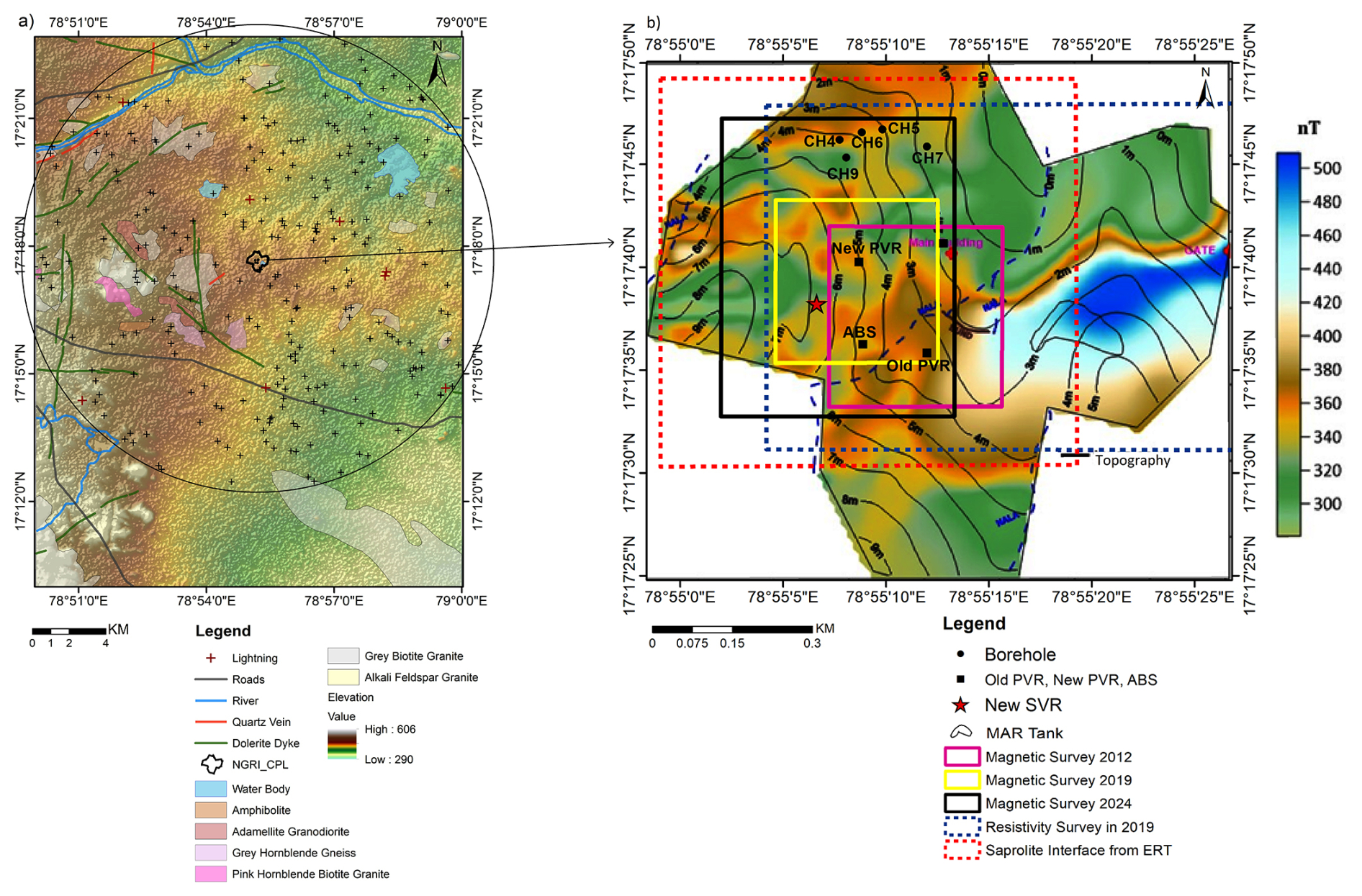
Figure 1 (a) The geological map shows the area around CSIR-NGRI-CPL observatory superimposed over topography. “+” symbols show lightning locations within a 10 km radius (circle mark) from January to August 2022, with a maximum intensity 60 480 A. (b) The magnetic anomaly map (after Sanker Narayan et al., 1967) is superimposed on local elevation. The locations of the magnetic and electric surveys are marked by solid and dashed rectangles. PVR = primary variometer room, ABS = absolute room, SVR= secondary variometer room, MAR = managed aquifer recharge.

The geo-electric measurements at CPL were based on orthogonal 500 m electric dipoles, and magnetic pulsations were measured with solid core induction coils. Hourly values of the magnetic variation and analysis of equatorial magnetic pulsations were reported from CPL (CSIR NGRI report, 1972). These hourly values are published in the Indian magnetic data volumes and uploaded to WDC Kyoto (Svendsen et al., 1990). Figure 1b shows the 42.5 ha, star-shaped campus of CSIR-NGRI located in Choutuppal, along with the marked locations of the primary variometer (PVR) and absolute (ABS) rooms. One high magnetic anomaly is present at the eastern part of the campus. In the rest of the area, the total range is ∼80 nT. The surface topography is least in the east and north and higher is the west and southern part of the campus. Several shallow boreholes drilled in the northern end are used for hydrogeological studies in fractured hard rock terrains. These studies monitored the nature of the granitic basement rocks, local hydrogeology and managed aquifer recharge (MAR) within CPL observatory, through a large, shallow lake in the eastern quadrant of the campus.

Geo-electric measurements on this campus were discontinued in 1982, but when the Metro Rail project in the vicinity of the HYB magnetic observatory in Hyderabad appeared to threaten its existence in 2010, the Choutuppal campus was re-visited for re-location possibilities of HYB. This work summarises the different situations, which affect the operation of a low-latitude magnetic observatory, some mitigation measures and some unanswered questions.

2 First phase of CPL magnetic observatory

2.1 Survey of magnetic data and building CPL Observatory

Prior to establishing the observatory buildings, a magnetic survey was conducted in November 2012 over an area of 200 m × 200 m with 20 m intervals, between the main building and the southern side of the campus, marked by the pink rectangle in Fig. 1b, which had the smallest anomalies as per the earlier survey. This area was sufficiently far away from the boundary of the campus to ensure that local activities outside the campus may not have significant contribution to the measurements. The total magnetic anomaly range (Fig. 2) was ∼ 150 nT with changes in magnetic field within ∼ 20 nT around proposed locations of the old PVR and ABS rooms.

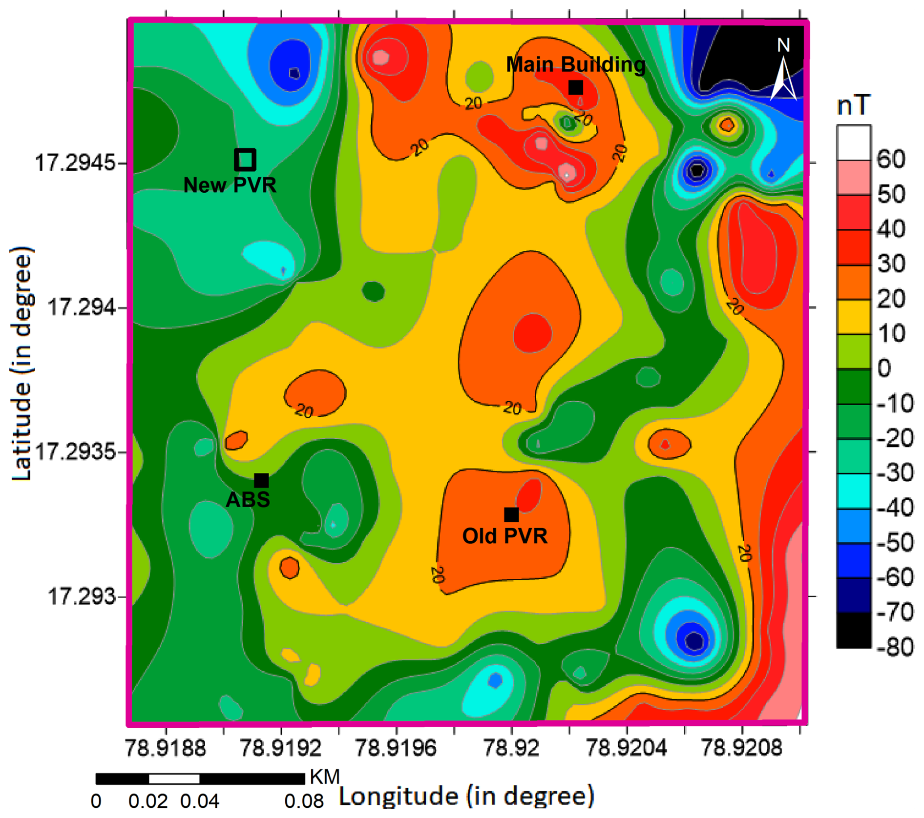
Figure 2 Magnetic anomaly plot of the survey region in 2012. Black box is the marked location for the New PVR, built in 2019–2020.

In this central location the surface topography is low, and a shallow water channel (nalla) flows SE–NW through the area between the old PVR and ABS. The old PVR construction (with double-walled, 3.5 m underground vault) started in June 2013 using non-magnetic sandstone. The ABS room was constructed on slightly elevated ground with two pillars inside and four pillars outside. In April 2014, CPL observatory was commissioned and equipped with a tri-axial fluxgate magnetometer and Zeiss single-axis fluxgate theodolite for declination–inclination measurements. The XVII IAGA Observatory Workshop was held on these premises in October 2014 with 93 international participants from 33 countries (Arora et al., 2016). The definitive data from CPL are published at INTERMAGNET (https://intermagnet.org/data_download.html) for 2015 onwards.

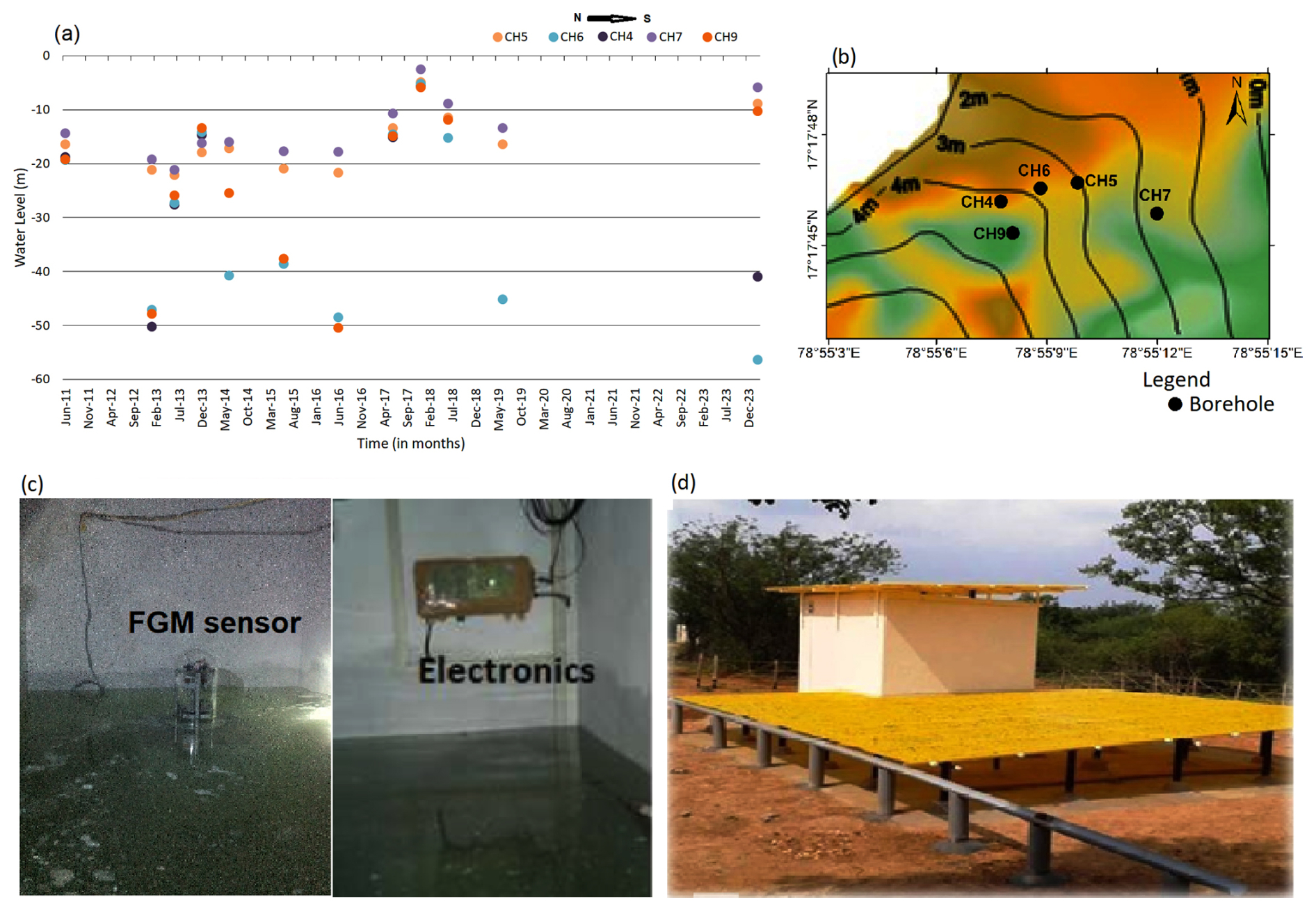
Figure 3 (a) Fluctuations of water level in a few boreholes in the north of Choutuppal campus, (b) location of boreholes in the map, (c) the submerged vault in September 2017 and (d) the outside view of the old PVR.

2.2 Hydrogeological park and managed aquifer recharge

The region of CPL observatory has a semi-arid climate with average annual maximum temperatures ranging as 28–45 °C. The mean annual rainfall is around 751 mm, which ranges from 2 mm in February to 171 mm in July. Water levels are highly variable depending on the monsoon and usually range between 2 and 26 m (metres below ground surface). Water level measurements at the northern part of the Choutuppal campus have been monitored since 1999 in two dozen boreholes (some of them are marked in Fig. 1b) by the Indo-French Center for Groundwater Research (IFCGR) (Maréchal et al, 2018) to study the hydrodynamic properties and associated hydrological processes in crystalline aquifers. As part of a governmental scheme of strengthening groundwater through recharge state-wise MAR projects, an infiltration basin was dug in Choutuppal (marked in black outline as MAR in Fig. 1b) in 2015 to meet the demands of farmers in the area facing water scarcity. The basin has dimensions of 120 m × 40 m, with a depth of about 2 m, effectively removing the regolith layer and extending into the saprolite. The basin is mainly supplied by a canal which diverts water from the Musi River (Nicolas et al., 2019; Maurya et al., 2021). Nicolas et al. (2019) have shown that intra-seasonal groundwater fluctuations only have a moderate response to rainfall patterns, which could be due to usage trends as well as hydraulic permittivity parameters. After the MAR basin filling, groundwater levels rose by 6 m in 1 year. Figure 3a shows the water level changes of five boreholes (CH5, CH6, CH4, CH7 and CH9) before and after the monsoon from 2011 to 2023, with a data gap during 2021–2022. While it is clear that most of the time water level lies at intermediate depth of ∼ 10 to 30 m, individually, CH5 and CH7 show the least seasonal fluctuations over the years, CH6, CH4 and CH9 show variations of 20 m or more; possibly very local fracture properties facilitate vertical flow of water. Starting from April 2017, the water levels in the boreholes rose significantly, coming almost to the surface in September 2017 and reducing a little by July 2018. In December 2023, the water levels recorded are nearly similar to those of September 2017. It can be inferred that sustained water in the MAR basin has allowed the shallow aquifers to be permanently recharged. In September 2017, the rainfall of the monsoon combined with prevalent saturated condition led to the flooding of the old PVR vault (Fig. 3c). The water level receded by a few metres the following summer but did not fall to earlier levels. While this was good news for recharge, the old PVR was now unusable.

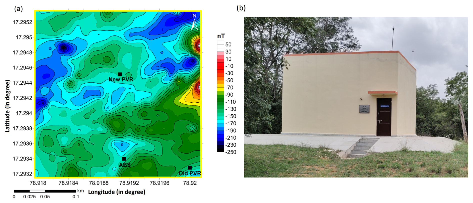
Figure 4 (a) Magnetic anomaly plot of the survey region in 2019 and (b) new PVR building inaugurated in January 2021.

3 Second phase of CPL magnetic observatory

3.1 Survey and commissioning of new PVR

With the need for a new variometer building, a fresh survey was conducted in May 2019 using GSM19 Overhauser magnetometers, marked by the yellow rectangle in Fig. 1b. This area was some tens of metres west of the earlier survey location, still central to the campus, on ground which is about 2–3 m higher, which could avoid the shallow groundwater conditions. This total field magnetic survey was carried out during 6 geomagnetically quiet days in May 2019 over a 240 × 240 m² area with 10 m spacing. The magnetic anomaly of the region shows total amplitude variation of ∼ 300 nT (Fig. 4a) with ∼ 10 nT anomaly north of the ABS room; the proposed location is marked as new PVR in Fig. 4a. This time a raised building with double walls and a double roof was constructed of non-magnetic limestone to ensure no groundwater incursion issues for the foreseeable future (Fig. 4b). The new PVR was commissioned in January 2021.

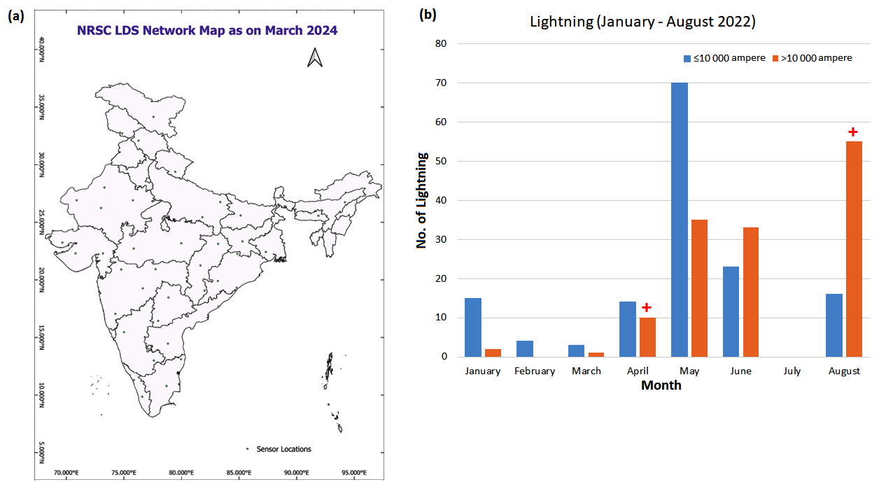
Figure 5 (a) Map of lightning sensors in India and (b) distribution of low- and high-intensity lightning occurrences during January to August 2022.

Recurrent malfunctions of the electronics (two to three times a month) of the digital fluxgate magnetometer (DFM) recording electronics were noticed in the second half of 2021 and 2022, a new phenomenon. After rounds of thorough inspections, it was suspected that lightning activity in the vicinity of the Choutuppal campus was causing the damage in spite of installation of six lightning arrester rods and four earthing pits. Being an open ground with no tall obstructions, the lightning activity in this area was found to be more frequent than around HYB observatory in Hyderabad. The earthing pits and lightning arrester system were strengthened further but only marginally countered the effects on the electronics.

3.2 Lightning activity patterns around CPL Observatory and effects on data

ISRO-National Remote Sensing Center (NRSC) has a network of 46 radio frequency lightning detection sensors, covering the entire part of the India (shown in Fig. 5a). The lightning detection sensor network monitors the cloud to ground lightning occurrences by virtue of emitted waves in the 5 Hz–30 MHz range, and geolocation is calculated using the time of arrival method. The detection range is up to 800 km, with more than 98 % confidence within 300 km range, with 50 % overlap to maintain high geo-location accuracy of lightning occurrences (Taori et al., 2022, 2023). We have examined the lightning data in a radius of 10 km around CPL observatory, marked as + in Fig. 1a. Figure 5b shows the shows the occurrence frequency of lightning over the months from January to August 2022; + symbols denote the instances when the lightning caused damage in the fluxgate electronics. Figure 5b shows that substantially lower intensity lightning activities are recorded during January, April, May and June. Surprisingly July had no lightning in the area in 2022, and in August, the higher-intensity lightning was more frequent. Two instances of failure of the instrument electronics occurred during the higher-intensity lightning of April and August, whereas a disturbance in May was associated with lower-amplitude lightning, discussed in the next section.

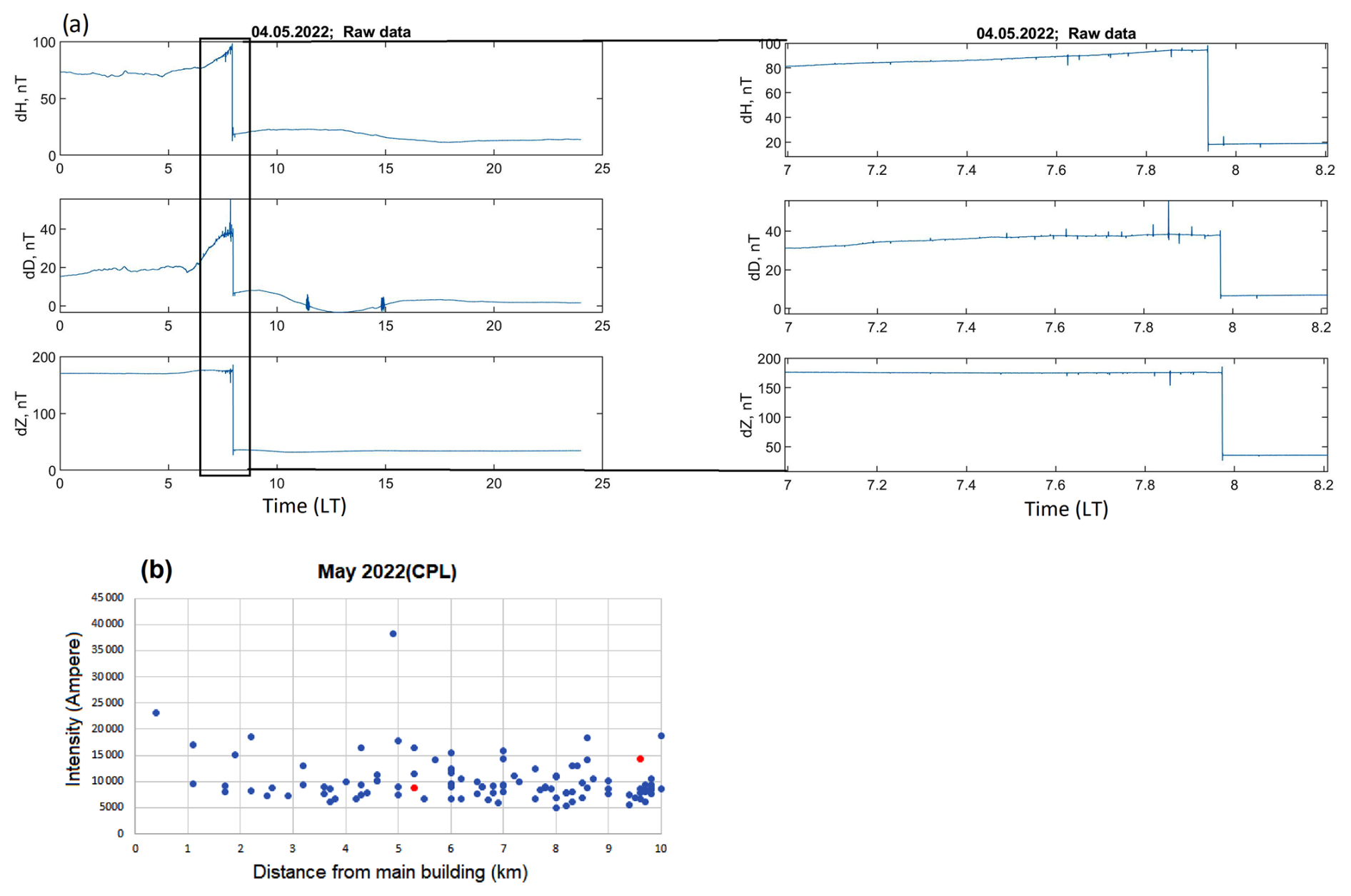
Figure 6 Raw data (H, D, Z component) plot for (a) 4 May 2022 at the new PVR and (b) plot of lightning intensity (in ampere) with distance (in km) from the main building.

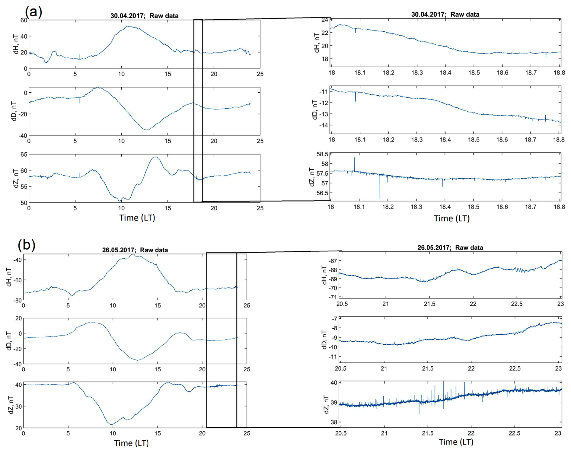
Figure 7 Raw data (H, D, Z component) plot for (a) 30 April and (b) 26 May 2017 at the old PVR.

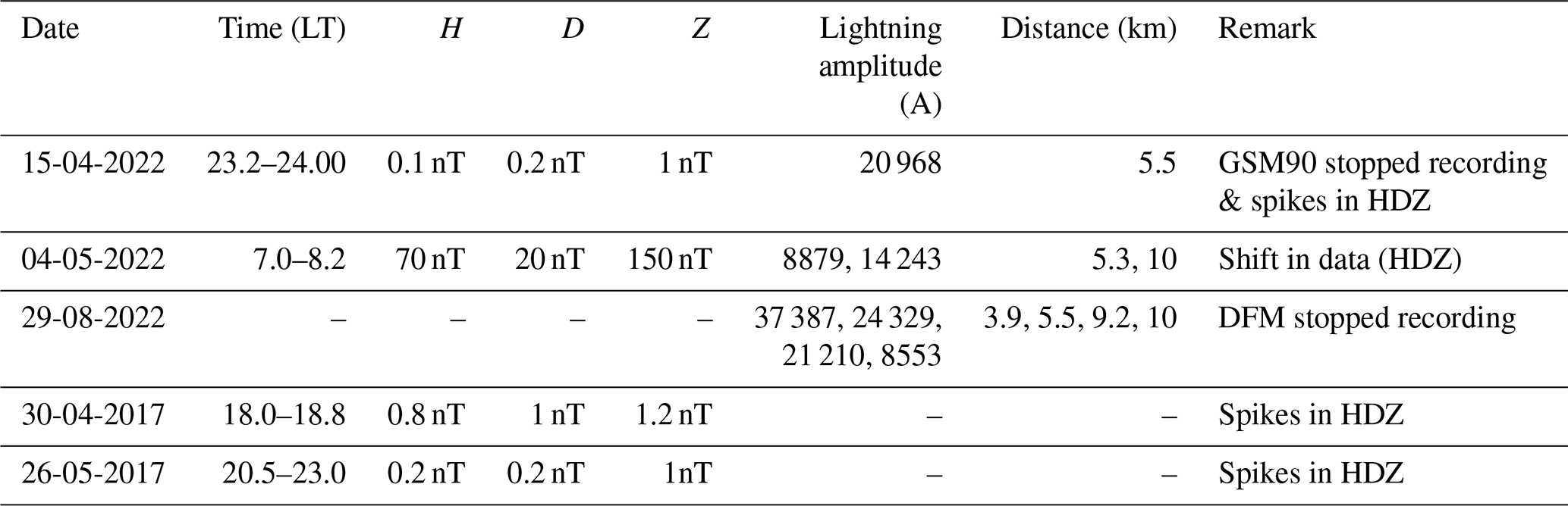
Examination of the H (horizontal), D (declination) and Z (vertical) components of 1 s data in LT (local time) for 4 May 2022 data from the new PVR shows continuous spikes from 7–8.2 LT in all the components, followed by a shift of ∼ 70, 20 and 150 nT in H, D and Z respectively (Fig. 6a). After rebooting the instrument, the data came back to their normal range. Comparison with lightning data established that this disturbance was due to the lightning effect (correlated red mark). It is noticed that at the time of 7.94 LT there was a shift in the data that correlates with the lightening intensity of 8879 and 14 243 A (ampere) at the same time, which struck the ground within 10 km radius of CPL campus.

Further, we examined the H, D and Z components of 1 s data in LT for the 30 April and 26 May 2017 data from the old PVR, on days which had some weather activities. From the data, it is clear that there were no shifts in the data, but some continuous spikes were observed from 18.0–18.8 LT (Fig. 7). The spikes are more prominent in the Z component (>0.5 nT). Though lighting data were not available in this duration, the general conditions lead us to believe that these minor signatures were lightning induced.

Table 1 Examples of the amplitudes of the disturbances recorded in data vis-à-vis the light intensities and distance from the recording system.

It was suspected that because the new PVR is constructed on the surface and the cables were laid in the surface layer, instead of the vault configuration as in the one which was flooded, the effects of lightning activity on the data have been amplified. Given the fact that in future years more uncertainty and swings in climatic parameters are anticipated due to the effects of climate change, it was deemed necessary to conduct further studies to find a location based on optimal ranges of a variety of parameters like topography, distance from MAR lake and the configuration of near-surface regolith and saprolite layers, along with groundwater conditions.

4 New search for optimal location

Higher ground away from the MAR basin can be found toward the western side of the campus. In order to evaluate its suitability as a new long-term location for continuous magnetic measurements, this study aims to delineate the subsurface structures using the high-resolution magnetic data constrained by resistivity information conducted through electrical resistivity tomography (ERT) and electrical vector resistivity imaging (EVRI) measurements at the Choutuppal campus and surrounding areas during 2016–2017. The magnetic method can be sensitive to the presence of near-surface variations and produce a model of these layers as well as in locating faults, folds, shear zones, delineating geological structures and groundwater contamination studies (Reynolds, 2011; Hinze et al., 2013; Kumar et al., 2018; Dwivedi and Chamoli, 2021, 2022). We try to find out a suitable location for a new SVR (secondary variometer room) where effects of lightning and groundwater level changes can be minimum in the medium to long term.

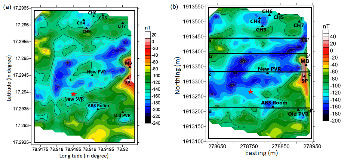
Figure 8 (a) The magnetic anomaly of the study area (MB = main building, SP = solar panel, CH = bore well channels, ABS = absolute, PVR = primary variometer room, SVR = secondary variometer room). Red star mark shows the proposed new SVR in the region, (b) the magnetic anomaly after reduced to equator of the study area. The aa', bb', cc' and dd' labels show four magnetic profiles modelled.

4.1 2024 survey

A 1 s total magnetic field survey was conducted during February 2024 (4 d) at 10 m sampling intervals as same done in 2019 survey. The data of 2019 and 2024 were combined, thus covering a total of ∼ 400 ×320  m². The diurnal and International Geomagnetic Reference Field (IGRF 14) corrections are applied to the F data, so that the residuals only reflect the local crustal contributions. Finally, we applied the kriging interpolation method to generate the grid and produce the magnetic anomaly of this area (Fig. 8a). Further, this was converted by a reduction-to-equator (RTE) computation to remove ambiguities in the location of causative sources of magnetic anomalies, at low and high latitudes. In this study, we chose the values of delineation =0° and inclination =24° and estimate the RTE-generated magnetic anomaly map of the study region. The RTE-filtered map centres anomalies over their sources and removes the asymmetry of the magnetic anomaly due to nonzero magnetic inclination and helps in magnetic data interpretation (Fig. 8b).

The RTE magnetic anomaly shows a variation of ∼ 260 nT in the region. The low anomaly is dominant in the central part, followed by the high anomaly near the main building and solar panel. The new PVR lies in the low-anomaly region where the three-axis flux magnetometer is installed to record 1 s H, D and Z component data of Earth's magnetic field. The ABS room location is set up in the low anomaly zone to measure the Delineation-Inclination using the Mag-01 DI-fluxgate magnetometer mounted on theodolite.

We have considered four profiles aa', bb, cc' and dd' along EW in the RTE magnetic anomaly map to characterise the subsurface susceptibility model (Fig. 8b). The magnetic data show their importance in characterising the shallow subsurface structures, which would be further beneficial for the selection of new location to install a magnetic observatory on the campus. The lightning data are considered from the National Remote Sensing Centre (NRSC), Hyderabad, India, to investigate the failure of the DFM (digital fluxgate magnetometer) electronics during the lightning strike. The high-resolution topography data are obtained from the Shuttle Radar Topography Mission (SRTM) Global 30 (https://earthexplorer.usgs.gov/, last access: 16 October 2024) to plot the elevation of the region.

The ERT surveys for different profiles (AA', DD', EE', FF' and GG') were carried out using Wenner and Schlumberger arrays with 48 electrodes in the campus. The profiles AA', DD' and EE' with 5 m unit electrode spacing achieved a maximum length of 360 m, whereas FF' and GG' cover 240 m (Maurya et al., 2021). The vertical cross-section along these profiles and a horizontal depth slice at a depth of 30 m below ground level (b.g.l.) derived from a 3D model reflect few linear conductive features and surficial resistivity heterogeneities (Fig. 13a).

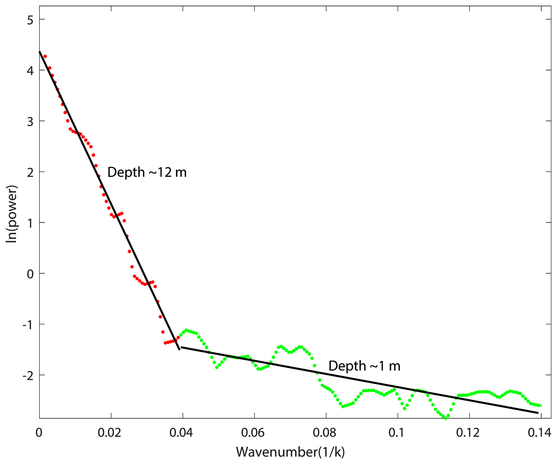
Figure 9 Radially averaged power spectrum of the RTE magnetic anomaly. Different layer segment gives an average depth of layered interfaces.

4.2 Analysis of subsurface source and depths

The fast Fourier transform (FFT) is a robust technique used by several researchers to calculate the mean depth of layered interfaces of the potential field datasets (Spector and Grant, 1970; Chamoli et al., 2011, 2023; Dwivedi et al., 2019). The power spectrum analysis gives the average depth of the sources with an error limit of 10 % (Mishra and Pedersen, 1982). The 2D radially averaged power spectrum of the RTE magnetic anomaly data shows two linear slope segments corresponding to the average depth of two interfaces around 12±1.2 and 1±0.1 m (Fig. 9).

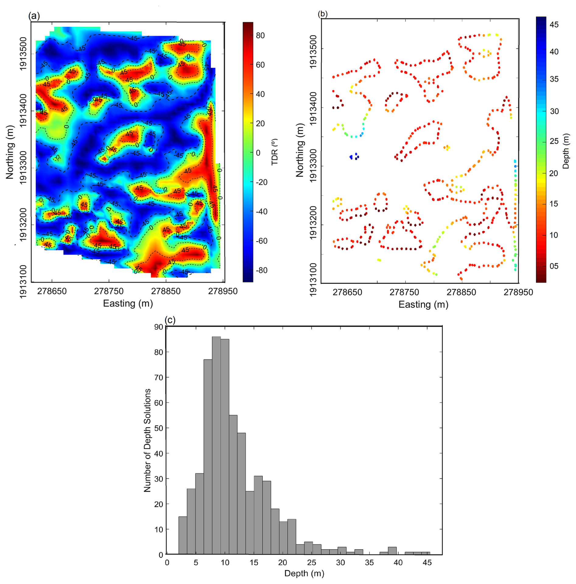
Figure 10 (a) The tilt angle plot, (b) the tilt depth solutions and (c) the tilt depth solution histogram plot of the RTE magnetic anomaly.

The tilt depth is an effective method in characterising the location of source edge as well as magnetic source depth using the tilt angle (TDR) approach (Salem et al., 2007). First, the TDR is described by the following equation (Miller and Singh, 1994):

$$\begin{array}{}\text{(1)}& \mathit{\theta }={\tan }^{-\mathrm{1}}\left[{\displaystyle \frac{\partial M}{\partial Z}}/\sqrt{{\left({\displaystyle \frac{\partial M}{\partial x}}\right)}^{\mathrm{2}}+{\left({\displaystyle \frac{\partial M}{\partial y}}\right)}^{\mathrm{2}}}\right],\end{array}$$

where $\frac{\partial M}{\partial x}$, $\frac{\partial M}{\partial y}$ and $\frac{\partial M}{\partial z}$ are the first derivative of the magnetic field M in the x, y and z directions. The zero contour (θ=0^°) demarcates the spatial location of the magnetic source, and tilt amplitudes are restricted in the range of +90° to −90°. Salem et al. (2007) introduced the tilt depth technique using the relationship among tilt angle (θ), depth (Z_c) and horizontal location (h) of a contact as

$$\begin{array}{}\text{(2)}& \mathit{\theta }={\tan }^{-\mathrm{1}}\left[{\displaystyle \frac{h}{Z_c}}\right].\end{array}$$

In Eq. (2), the contact location (h=0) lies at the zero values of the contour, and depth relates to the horizontal distance between the 0° and ±45° contour in the TDR map. We apply the technique to generate the tilt angle (TDR), tilt depth solution and histogram plot on the magnetic gridded data. Figure 10 presents the TDR map displaying contours of −45, 0 and +45° (dashed black lines). The TDR shows the short-wavelength anomalies and closely spaced contours that correspond to shallow subsurface sources. The zero contour values of the TDR show the location of the source, whereas the half of the distance between ±45° contours demarcates the depth of the sources. It can be seen that the distance between 0 and +45° is demarcated by relative closeness over the shallow sources and wide expanses over the deeper sources.

The tilt depth solutions of the RTE magnetic anomaly data with depth vary from ∼ 2 to 45 m. Most of the sources lie in shallow depths of ∼ 2 to 20 m and are extended in one direction. The histogram plot shows the variation between the number of depth solution and the depth (Fig. 10c). It is clear from the plot that the number of depth solution is maximum in the depth range of ∼ 2 to 20 m, which corresponds to the shallow source in the subsurface.

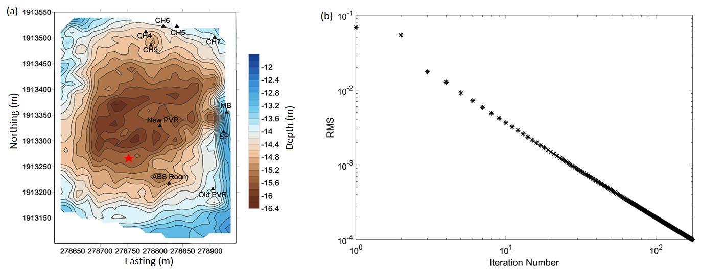
Figure 11 (a) The depth variation of the saprolite interface derived from the inversion of the RTE magnetic anomaly after removing the high-frequency component and (b) variation of RMS error against the iteration number.

4.3 Magnetic data inversion and forward models

We invert the RTE magnetic anomaly to estimate the depth variation of the interface with strong susceptibility contrast. We use the method of Parker (1973), which works in the Fourier domain to estimate the depth variation of an undulated interface. The depth of interface can be computed from the magnetic anomaly due to an uneven, uniform magnetised layer by inversion procedure. The method is improved by incorporating a high-cut filter to ensure the convergence of series and to avoid instability at high wavenumber (Pham et al., 2020). Based on the power spectrum characteristics, we have chosen the cut-off wavenumber between 0.038–0.13 m⁻¹ to remove the high frequencies. The resultant map shows that this interface is deepest in the centre of the survey area and shallowest towards the edges; then the present PVR and the ABS Room are in the zones where this interface is deep, whereas the old PVR which was flooded was in the zone of shallow interface (Fig. 11a). The calculated depth is inferred as the saprolite layer, which varies from ∼ 12 to 16 m with a mean depth of ∼ 14 m. Figure 11b shows the variation of the root mean square (RMS) error against the iteration number. In this case, the inversion process performed 175 iterations, and the RMS error between two successive approximations was reduced from 0.0680 m to $\mathrm{9.9584}\times {\mathrm{10}}^{-\mathrm{5}}$ m.

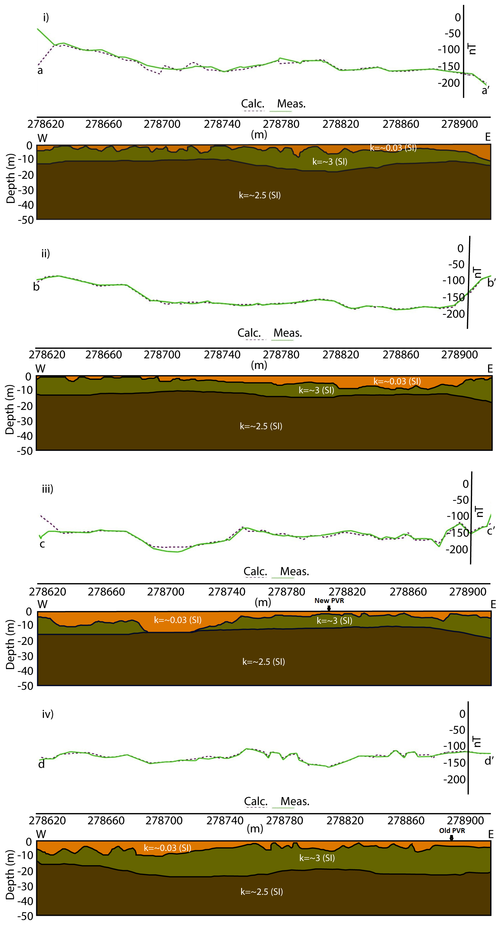
Figure 12 Magnetic data modelling across the profiles (i) aa', (ii) bb', (iii) cc' and (iv) dd' incorporating constraints from the power spectrum and past ERT studies. Top, middle and bottom layers in the models are sandy regolith, saprolite and granitic basements. The marked arrows show the location of new and old PVR in profile cc' and dd'.

Further, we model the RTE-derived magnetic anomaly data along four profiles, aa', bb', cc' and dd' (Fig. 8b) to delineate the details of the subsurface structures. The forward modelling along these profiles is carried out using the IGMAS+ software, a tool for forward and inverse modelling of potential field datasets (Anikiev et al., 2023). The total length of theses profiles is ∼ 310 m, which shows the depth variations up to 50 m from the surface (Fig. 12a). The 2D models along these profiles explain the presence of three layered structures from the surface up to a depth of 50 m as sandy regolith (∼ 0.3 susceptibility in SI), saprolite (∼ 3 susceptibility in SI) and fissured granite (∼ 2.5 susceptibility in SI). The average susceptibility value for the sandy regolith layer is measured in the field using a KT-10 magnetic susceptibility meter, whereas others are referenced from Telford et al. (1990). The saprolite interface is incorporated in the models based on previous results of ERT data (Nicolas et al., 2019). The average thickness of the sandy regolith layer is ∼ 3 m, whereas the saprolite layer is ∼ 10 m in the models. Both the saprolite and regolith layers show undulations in the all models.

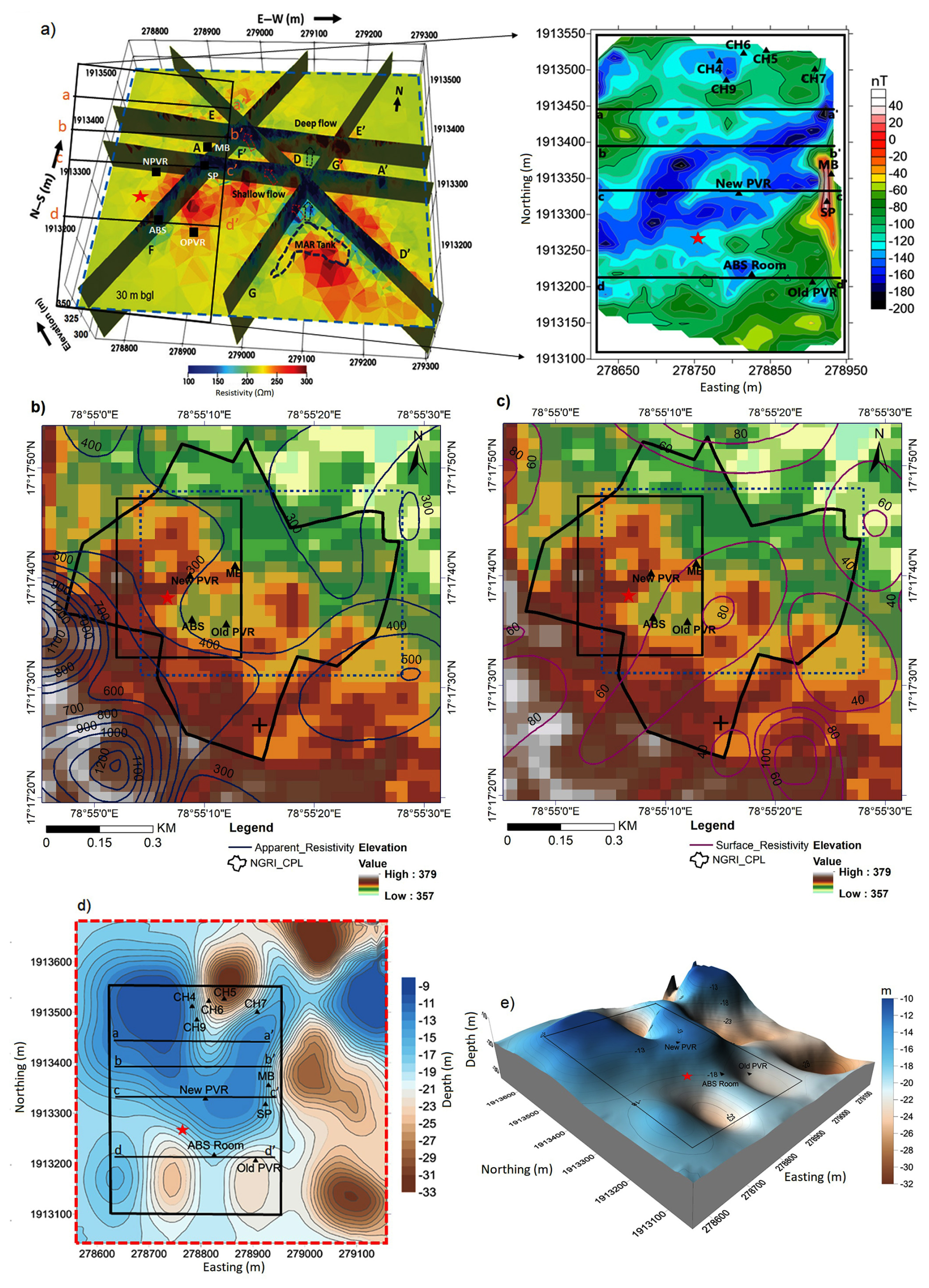
Figure 13 (a) A resistivity model of the 2019 profiles along AA', DD', EE', FF' and GG' and a depth slice at 30 m b.g.l. (after Maurya et al., 2021), (b) apparent resistivity, (c) surface resistivity superimposed over the topography with lightning strike location (+ symbol, intensity of 23 208 A at a distance of 400 m from the MB on 4 May 2022), (d) depth estimation of saprolite interface from ERT data (after Nicolas et al., 2019) and (e) 3D view of saprolite interface. The blue and red dotted rectangles represent the areas corresponding to the resistivity model and the saprolite interface, respectively, while the black rectangle highlights the magnetic anomaly region.

4.4 Correlation with conductivity data/information

The cc' magnetic profile is close to the vertical resistive cross-section along AA' of Maurya et al. (2021), where resistivity increases from surface to depth (Fig. 13a). The old surface and apparent resistivity data of the region are digitised from the Sanker Narayan et al. (1967) and overlaid over the topography (Fig. 13b, c). The apparent resistivity shows lateral varying high resistivity outward and vice versa inside the Choutuppal campus (Fig. 13b). This indicates that conductivity decreases outward, highlighting the presence of conductive soil layers within the campus.

The saprolite depth calculated by inverting magnetic data at different locations is ∼ 15.5 m (new PVR), ∼ 15 m (ABS Room and CH9), ∼ 13 m (MB and SP), ∼ 14 m (old PVR, CH5, CH6, CH7) and ∼ 14.5 m (CH4) (Fig. 11a), whereas depth estimation by the ERT data is ∼ 13.5 m (new PVR), ∼ 18 m (ABS Room), ∼ 15 m (CH9), ∼ 14 m (MB, SP and CH4), ∼ 22 m (old PVR and CH6), ∼ 29 m (CH5) and ∼ 17 m (CH7) respectively (Fig. 13d). The calculated depth from these two different datasets shows a discrepancy of ∼ 2 m, except at the locations of CH5, CH6 and old PVR. The ERT survey estimates the upper fissured layer depth (∼ 9 to 33 m) of the Choutuppal campus and shows the undulated interface creating compartmentalised aquifers (Nicolas et al., 2019).

5 Discussion and conclusion: proposed optimal location for SVR

The high-resolution magnetic data provide a detailed shallow subsurface structure at CPL observatory. The power spectrum result shows two segments at a depth of ∼ 12 and ∼ 1 m corresponding to saprolite and sandy regolith interface. These depths are similar to the previous depth estimated using the drilling data by Dewandel et al. (2006). The inversion results show the depth variation of the saprolite interface ∼ 12 to 16 m (Fig. 11a), which is underestimated when compared to the upper fissured layer depth from the ERT survey (Fig. 13d). The obtained interface shows depression in the central region of the map with crests in the outer region and linear variation in depths (Fig. 11a). The estimated depths at different locations show ∼ 2 m differences from these two datasets except at the location of CH5, CH6 and old PVR. These discrepancies in the depth estimation may be due to measurements of two different independent physical parameters susceptibility and conductivity. The saprolite interface might be delineated better by the ERT data due to presence of significant resistivity contrast between saprolite and granitic bedrock in the region (Robinson et al., 2008; Gourdol et al., 2021). The tilt depth plot of the anomaly data reflects depth variation from ∼ 2 to 45 m (Fig. 10b). The histogram plot confirms the presence of the shallow sources in the depth range of ∼ 2 to 20 m based on the majority of a number of depth solutions (Fig. 10c). These shallow sources are in circular and elongated shapes, which may be residue of igneous intrusion (Gorczyk and Vogt, 2018). At shallow depths, circular bodies with a magnetic contact source might produce symmetric anomalies in the magnetic data (Hinze et al., 2013). In contrast, elongated bodies may produce linear magnetic anomalies that follow the direction of the body as in the present study.

The subsurface susceptibility models along the magnetic profiles aa', bb', cc' and dd' reflect the geometry of the sandy regolith, saprolite layer and basement fissured granite (Fig. 12). The saprolite layer shows undulating variation with considerably thick and thin depths at different locations along the profiles. These variations illustrate that the saprolite layer is thin in the region where the anomaly is low, and it shows the thickness in the region where the anomaly is high. The magnetic anomaly shows a large depression of length ∼ 80 m in the profile cc' where the saprolite layer is absent, and this depression arises due to the sandy layer in the model. The 3D cross-sectional resistivity model infers the presence of high-conductivity anomalies followed by the moderate conducting saprolite layer and the low-conductivity basement rocks (Fig. 13a).

Figure 13b shows that the apparent resistivity increases laterally outward, indicating the presence of highly conductive soil layers within the campus (Sanker Narayan et al., 1967). The apparent and surface resistivity demonstrate the linear relationship with the topography. The comparison between the latest resistivity model (∼ 200 Ωm variation) for 2019 profiles (Fig. 13a) and the old apparent resistivity (∼ 300 Ωm variation) plot in 1964 (Fig. 13b) shows the resistivity change of ∼ 100 Ωm. This discrepancy may be due to the presence of a newly constructed artificial recharge pond, which may decrease the resistivity due to its high-conductivity nature. The thin saprolite layer may be associated with high electrical conductivity, which can result in a low magnetic anomaly, and vice versa. Overall, the resistivity variation increases from surface to greater depth. The resistivity model also shows that the artificial recharge pond has good subsurface connectivity, helping the groundwater recharge towards the north and northwest directions in the campus (Maurya et al., 2021). The water level started to rise in June 2016 and reached very shallow depth in channels during December 2017. It is evident that since the last half of 2016, the recharge has led to saturation, which transformed the hydrogeological regime of the campus. This may also cause a partial change in the rock magnetism due to water saturation (Csontos et al., 2019), resulting in a decrease in the magnetic anomaly (Figs. 4a, 8a). The rainfall of the 2017 monsoon combined with the already prevalent saturated conditions led to the flooding of the magnetometer vault. The location of new PVR has advantages as it is away from the water recharge pond and has a minimal magnetic anomaly but generates an induced current in the rainy seasons due to the presence of the conductive environment around the location. The effect of lightning strikes on the data with increasing distance, intensity and ground conductivity shows that higher-intensity strikes have had an impact on the data and instruments.

Based on the above it is very crucial to determine the location and configuration whereby the installation can avoid the effects of groundwater fluctuations as well as lightning strikes, based on the nature of subsurface rocks, soil conditions and their magnetic variations. The susceptibility model, along with resistivity information, is used to make a selection of a new SVR (78.9185° E, 17.2939° N), indicated by the red star in Figs. 1, 8, 11 and 13. This location has a low magnetic anomaly of $\sim -\mathrm{145}$ nT (Fig. 8a), resistivity ∼ 200 Ωm (Fig. 13a), moderately high ground ∼ 367 m (Fig. 13b) and a depth of the saprolite layer of ∼ 20 m (Fig. 13d). A thicker saprolite layer can enhance the resistive environment and reduce current propagation. The location's sufficient distance (∼ 320 m) from the recharge tank ensures that water infiltration is unlikely to pose a significant issue. It is proposed that the pillar will be constructed within a semi-underground vault, in order to minimise the influence of induced currents during rainy seasons and lightning strikes. Additionally, the volume surrounding the pillar should be filled using a high-resistivity material, such as quartzite, to further minimise the likelihood of induced currents during lightning events or wet conditions.