A user-orientated column modelling framework for efficient analyses of the Martian atmosphere

As spacecraft missions return ever more data from Mars, additional tools will be required to explore and analyse these datasets efficiently. To streamline research into the atmosphere of Mars, a user-orientated modelling capability is developed that enables automatic initialisation and running of a column model.

As a demonstration we utilise the modelling framework to provide additional verification for the University of Helsinki and Finnish Meteorological Institute Mars column model temperature profiles above the height of typical lander meteorological measurements, i.e. above 2 m. We utilise the framework at landing site locations that are well characterised to understand the model's applicability and to identify future opportunities for modifications to the framework. We do this by using the framework to compare the column model to temperature soundings made by the Mars Reconnaissance Orbiter.

We find that the column model, without any modification, is able to reproduce the observed lapse rates and average temperatures closely in most cases except for a 20–60 K increase over the northern hemisphere mid-winter. We can reproduce this discrepancy by incorporating an adiabatic heating term into the column model. Fitting of the modified column model to the observations results in estimated maximum downward vertical wind velocities of ∼ 10 cm s⁻¹ at altitudes of 15–20 km over the winter solstice at the VL-1 and VL-2 sites. The approach developed here may possibly provide a way to independently estimate or observe the vertical motion in the Martian atmosphere. However, even though the magnitude of the vertical wind speed appears reasonable, it is not clear at this point how much the atmospheric heating is due to other mechanisms such as advection.

We have introduced new application software that can quickly find and display the requested data and can be immediately analysed using the included tools. We have demonstrated the potential of this type of software application with a glimpse into the upper atmosphere of Mars.

1 Introduction

Observational data are being returned from Mars in ever increasing quantities by spacecraft. To manipulate these data and compare them with the vast amounts of data generated by computer models, specialised software tools are required. Tools for searching, extracting and visualising the relevant data have been made readily available by the space agencies. Exploration of these large datasets, if stored online, can be time consuming and important data may be missed due to time constraints. Ideally the data need to be stored on a host machine and accessible via a local network with a fast connection or to be stored on the same work station that is being used for analysis. This then requires the integration of tools into a single software package to query the database and analyse the data.

Column models of the Martian atmosphere are a fast and convenient analytical tool for investigating the lower sections of the Martian atmosphere, i.e. below the planetary boundary layer or below 5–10 km altitude. With a suitable radiation scheme they can accurately model the temperature in the lower part of the atmosphere (Savijärvi et al., 2005). A 1-D model can be particularly well suited to investigating the Martian atmosphere at specific locations such as landing sites. This is because the radiative timescale of the atmosphere (1–2 sols) is short, making it relatively insensitive, compared to Earth's atmosphere, to horizontal heat transfer through advection.

At particular times of the year and at certain locations, the atmosphere deviates from radiative equilibrium, e.g. during the northern hemisphere winter, as warm air is generated by adiabatic compression in the descending arm of the meridional circulation (Heavens et al., 2011). This can create a significant temperature inversion up to an altitude of between 10 and 20 km at middle to high latitudes. The magnitude of this temperature inversion may be controlled, to some degree, by radiative forcing from atmospheric dust. When using a column model, care then needs to be taken to make sure any large-scale dynamical processes are not interfering with the interpretation of the results from the model. Alternatively, a term could be included in the model to account for the adiabatic heating.

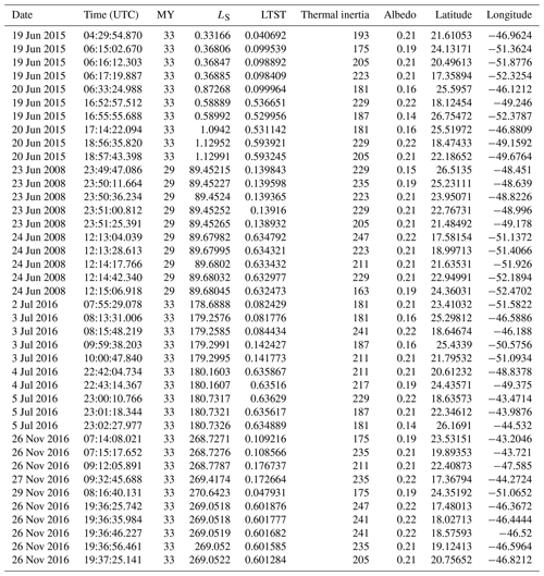
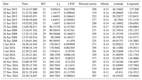
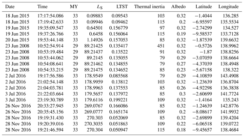
In the next section we describe a column model and satellite soundings in the Martian atmosphere. In Sect. 3 we give a system-level overview of the software application and describe its operation. In addition, we introduce an adiabatic heating adjustment for the model. In Sect. 4 we demonstrate the use of the application and verify the column model. In Sect. 5 we discuss the reasons for differences between the column model results and the soundings. Tables of the times, locations, thermal inertia and albedo for individual vertical profiles can be found in the appendices.

2 Background

The University of Helsinki and the Finnish Meteorological Institute (UH/FMI) have developed a column model that has been extensively used to investigate the planetary boundary layer at Mars including surface–atmosphere interactions (Savijärvi et al., 2004, 2005, 2018; Savijärvi, 1999, 1995; Savijärvi and Kauhanen, 2008; Savijärvi and Määttänen, 2010; Paton et al., 2016). The model includes time-stepping calculations for wind, temperature, specific humidity and ice mixing ratio. It includes long- and short-wave radiation schemes taking into account atmospheric CO₂-H₂O and dust. For turbulence a Monin–Obukhov scheme is used for the lowest layer and a mixing approach aloft. Energy balance at the surface uses a Crank–Nicolson method to calculate the surface temperature. Surface ice and adsorption is also modelled.

The Mars climate sounder (MCS) aboard the Mars Reconnaissance Orbiter has been observing the temperature, humidity and dust content of the Martian atmosphere from 2006 onward. The instrument views Mars through eight thermal infrared channels and one spectral channel with a total of 21 detectors (Joyner and Sayfi, 2012; McCleese et al., 2007). The standard viewing strategy for MCS is to observe along its direction of travel from a polar orbit. Limb and nadir observations are made in succession during each sounding acquisition with the nadir observation providing near-surface information on the atmosphere. The typical vertical resolution provided by the individual sensors is around 5 km. A vertical resolution of about 1 km is available on the Planetary Data System together with appropriate errors. See Kleinböhl et al. (2009) for details on the retrieval process. The polar orbit enables MCS to acquire one morning (∼03:00 LTST, Local True Solar Time) and early afternoon (15:00 LTST) sounding from each latitude and longitude on Mars.

3 Method

3.1 Description and operation of the framework

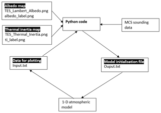
A prototype framework was developed to enhance data exploration operations by the addition of an in-line analytical dimension to the process. The framework works by searching observed data using a filter while at the same time analysing the data by comparison to a column model. Figure 1 shows an overview of the software architecture of the framework developed for this purpose. The data we wished to search and examine were observations of atmospheric temperature made by MCS and our main analytical tool was the UH/FMI column model. A Python wrapper used for implementing user actions via a graphical user interface (GUI) was especially developed for this project. The Python wrapper also includes the code for manipulating the data.

Figure 1 Software, files and data paths used by the application.

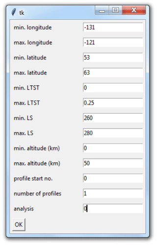
Figure 2 Screen capture of the framework's GUI form that features the input fields used for searching the data. The last input field is for choosing an analysis option. The user enters the minimum and maximum bounds of the search parameters into the input fields. Longitude and latitude are the coordinates of the temperature profile of interest. Local True Solar Time (LTST) is the time of the temperature profile. LS is the areocentric longitude in degrees when the profile. Altitude is the altitude of the lowest point available in the profile, i.e. the lowest point of the profile needs to be in the min. or max. range entered in the altitude fields. The “profile start no.” input field indicates at what point in the search results to begin any output. The “number of profiles” indicates the number of profiles in the search results that should be output. The “analysis” input field options are described in the main text.

The Python code is organised into three components. The first component contains the GUI (Fig. 2) and performs the basic operations activated by the GUI. The second component contains the data processing and analysis tools required for performing the main functions of the application. The third component contains the database tools for fetching and storing the data for easy access by the application. The database framework also allows for easy expansion of the database.

The GUI, as shown in Fig. 2, is constructed as a form with input fields allowing keyboard entry of ranges for searching the MCS data. The input field, at the bottom of the form, is used for selecting the type of analysis that the user wishes to perform on the MCS data. Entering “0” for the analysis performs a search based on the entered parameters and returns the number of profiles available in the Python console. Further details, such as time, locations, lowest temperature etc., are written to a text file. Entering “1” plots the MCS temperature profile together with the atmospheric temperatures from a corresponding model run and is displayed in the Python console. Fitting of the model to the observations by automatic variation in the vertical wind speed can be requested by entering a “2”. Other fitting operations are possible, such as variation in optical depth (tau), surface albedo and thermal inertia, although their utility have not been ascertained at the present time as the MCS temperature profiles do not generally reach close enough to the surface. See Appendix B for more details on the working environment and some examples of output from the framework.

The initialisation file for the column model is assembled by the Python wrapper from a number of sources. The model initialisation file contains the values for the following parameters: areocentric longitude, time of day, surface temperature, surface pressure, latitude, thermal inertia, albedo and optical depth (tau). The Python wrapper places all the model initialisation values in the output file, “Output.txt”.

The sources for the values found in the output file are as follows. The areocentric longitude and time of day is extracted from the MCS profile header. The wrapper obtains the surface temperature and pressure values by the extrapolation of the pressure and temperature values from the lowest point that if finds in the MCS profile. The longitude and latitude of the profile is obtained from the profile header. The profile location is then used for extracting the thermal inertia and albedo data from maps of TES (Thermal Emission Spectrometer) observations. The optical depth (tau) for the initialisation file is currently hard coded into the Python wrapper but can be adjusted manually (see Appendix B for a description of the working environment). Currently the parameter, τ, is adjusted manually based on data from the Mars Climate Database (MCD) web interface, depending on the location and time of year, although this will most likely be automated in the future.

The Python wrapper receives the results from the column model via an input text file that contains the altitude of the model atmospheric grid points and the associated temperatures. There are 28 model grid points and they increase exponentially for efficient computation. The grid points are as follows: 0, 0.3, 1.0, 1.6 … 7000, 10 000, 14 000, 20 000 and 28 000. Extra grid points can be added or adjusted in principle. However, we use this configuration of the model as it has been used in previous work and its operation is well known.

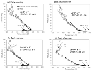
Figure 3 Viking Lander 1 site temperatures observed by the Mars climate sounder together with temperatures from the column model. Five MCS soundings are plotted in each figure. The profile locations range from latitudes between 17 and 27^∘ N and longitudes between 43 and 53^∘ W. The range of solar longitudes and local times are indicated in the legends for each set of profiles. Early morning and afternoon profiles are plotted for the spring equinox and the summer solstice. Plots for subsequent seasons can be found in Fig. 4. Also shown are the VL-1 1.6 m altitude temperature measurements and inferred surface temperature from Paton et al. (2016). Overlaid, as a check, are data from the MCD. See Appendix A for a table listing details of each sounding and input data for the model. Mars year 29 (Earth year 2008) for $L_{\text{S}}=\mathrm{90}{}^{\circ }$ and Mars year 33 (2015–2016) used for all areocentric longitudes.

3.2 Adiabatic heating modification for the column model

Column models do not as such include vertical motion in their calculations. For the present application, a simple but realistic approximation of adiabatic heating (Holton, 2004) due to the systematic downward motion in the meridional Hadley cell was added to the model. Its temperature tendency equation then reads (with horizontal advection omitted)

$$\begin{array}{}\text{(1)}& {\displaystyle \frac{\partial T}{\partial t}}=-w\left({\mathrm{\Gamma }}_{\text{d}}-\mathrm{\Gamma }\right)+Q_{\text{rad}}+Q_{\text{turb}},\end{array}$$

where $\mathrm{\Gamma }=-\text{d}T/\text{d}z$ is the actual temperature lapse rate (by finite difference at each time step and altitude point) and Γ_d is the constant adiabatic lapse rate, which is 5 K km⁻¹ on Mars. The other right-hand side (RHS) terms are due to radiation and turbulence. Vertical velocity w(z) must now be provided as an extra parameter.

The assumed structure used to represent a typical profile of the vertical wind is based on the MCD profiles, e.g. see Fig. 9, with a parabolic function for the upper part and the formula for a circle on the lower section.

$$\begin{array}{}\text{(2)}& w_{\text{top}}=-f_z{\displaystyle \frac{v_z-v_l}{\mathrm{400}}}{\displaystyle \frac{z\left(j\right)-z_l}{\mathrm{1000}}}\left[f_z{\displaystyle \frac{z\left(j\right)-z_l}{\mathrm{1000}}}-\mathrm{40}\right],\end{array}$$

where f_z is a factor that controls the width, i.e. vertical distance between the two arms, of the parabolic function; v_z is the maximum vertical wind speed; v_l is the vertical wind speed at which point the w_low function (see below) begins or is “linked” to w_top; and z_l is the altitude at which w_low begins.

$$\begin{array}{}\text{(3)}& w_{\text{low}}=v_l-v_l{\left[\mathrm{1}-{\displaystyle \frac{z(j{)}^{\mathrm{2}}}{z_l^{\mathrm{2}}}}\right]}^{\mathrm{0.5}}.\end{array}$$

The fit parameter for comparing the modified model to the soundings is calculated as follows:

$$\begin{array}{}\text{(4)}& T_f^{\mathrm{2}}=\sum _{n=\mathrm{1}}^{\mathrm{5}}{\left(T_n-S_n\right)}^{\mathrm{2}},\end{array}$$

where T_n is the temperature from the model, S_n is the temperature from the MCS sounding and n is the index for the altitude of the temperature. The model and observations are compared at the model grid point altitude levels of 7000, 10 000, 14 000, 20 000 and 28 000 m corresponding to index numbers n=1, 2, 3, 4 and 5, respectively. At these altitudes, which correspond to grid points in the model, the observations diverge the greatest from the model over the winter solstice, see Fig. 6d. A hill-climbing algorithm was used to vary the profile coefficients $f_z,v_z,v_l$ and z_l once each sol. This was only used over the winter solstice when the observed temperatures diverged significantly from the model. The column model repeated the temperature calculation for the sol until T_f was below a predefined threshold that was set taking into account accuracy and running time constraints. The threshold temperature was set at 3 K giving a fitting error of around 1–2 K for each point in Fig. 6.

The column model was spun-up over 4 sols to enable the upper atmosphere to reach equilibrium. The sol used for fitting was then the fifth sol.

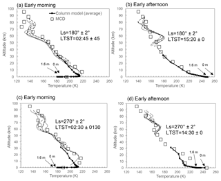
Figure 4 VL-1 site MCS temperature soundings and model temperatures compared. As for Fig. 3 but for the autumn equinox (L_S180^∘) and the winter solstice (L_S270^∘). Five MCS soundings are plotted in each figure. See the caption of Fig. 3 for preceding seasons and details regarding the profile locations and an explanation of the legends. Also shown are the 1.6 m altitude temperature measurements and inferred surface temperature from Paton et al. (2016). Overlaid, as a check, are data from the MCD.

4 Verification of the column model

The column model was first verified, without the adiabatic heating adjustment introduced in Sect. 3.2, by comparing it to temperature profiles made by MCS. The MCS data were searched for temperature profiles around the Viking lander 1 (VL-1) landing site, the Viking lander 2 (VL-2) landing site and Mars Science Laboratory (MSL) landing site using the new tool described in Sect. 3 to compare with and to verify the column model. Temperature profiles were also obtained independently, i.e. manually, from the MCD web interface (Lewis et al., 1999) as an additional check. The parameters used to search the MCS data were longitude, latitude, solar longitude and local time. A range of ±5^∘ around each site's longitude and latitude coordinates was required to obtain a sufficient number of profiles. For areocentric longitude the range was searched between L_S ±10^∘ and Local True Solar Time (LTST) 0 to 0.25 for morning soundings and 0.25 to 1.0 for afternoon soundings. The values for optical depth (tau) were estimated from MCD, thereby taking into account seasonal and areal distributions in dust. Values for tau of 0.4 were estimated for VL-1, VL-2 and MSL except during the northern winter solstice when a value of 1.0 was used for VL-1 and MSL.

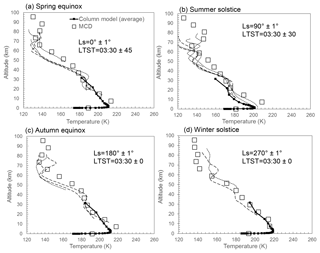
Figure 5 MSL site night-time atmospheric temperatures observed by the Mars climate sounder together with temperatures from the column model. Overlaid, as a check, are data from the MCD. As for Figs. 3–4 but for the MSL site (4.6^∘ S, 137.4^∘ E). Mars year 29 (Earth year 2008) for $L_{\text{S}}=\mathrm{90}{}^{\circ }$ and Mars year 33 (2015–2016) used for all areocentric longitudes.

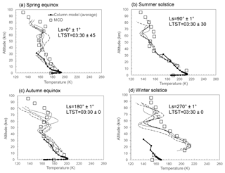
Figure 6 VL-2 site night-time atmospheric temperatures observed by the Mars climate sounder together with temperatures from the column model. Five MCS soundings are plotted in each figure. Overlaid, as a check, are data from the MCD. As or Figs. 3–4 but for the VL-2 site (48.0^∘ N, 134.3^∘ E). Mars year 29 (Earth year 2008) for $L_{\text{S}}=\mathrm{90}{}^{\circ }$ and Mars year 33 (2015–2016) used for all areocentric longitudes.

Figures 3–6 show the temperatures retrieved from the MCS data together with the results from the column model runs, which were initialised with information specific for each case. Overlaying the figures are climate model temperatures from the MCD. Many of the MCS soundings do not reach the surface as the lower segments of the profile are rejected due to the various selection criteria used to judge a successful retrieval (Kleinböhl et al., 2009). Tables listing times, locations, thermal inertia and albedo for each sounding used can be found in Appendix A.

The MCS temperature soundings in Figs. 3–6 are somewhat similar to each other despite being retrieved over a large region, with diverse surface properties, surrounding each landing site. The similarity in temperature profiles above about 10 km is consistent with global circulation model (GCM) results and observations that suggest the temperature in this region of the atmosphere is largely controlled by the large-scale circulation of the climate. Below 10 km, in situ wind measurements (Paton et al., 2018) also indicate good agreement with GCM results in terms of wind direction, perhaps reflecting the influence of the large-scale circulation. However, wind speed is less consistent with GCM results, perhaps reflecting some local influences from variations in topography or surface thermal properties at these altitudes.

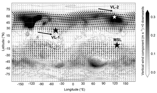
Figure 7 MCD vertical velocity w and horizontal winds at an altitude of 20 km at an areocentric longitude of $L_{\text{S}}=\mathrm{270}{}^{\circ }$. The convention used here is opposite to the one we used in Sect. 3.1. Note, to make visualisation of the downwelling regions clearer only the positive downwelling velocity is shown. Any negative velocities are white. The long arrows next to the VL-1 and VL-2 sites represent the direction of the winds immediately to the west of those sites.

Due to the lack of full coverage down to the surface from MCS, it is difficult to compare individual plots to each other. It is apparent though that column model, soundings and MCD are in broad agreement with the observations. Both the soundings and the MCD tend to be slightly warmer than the column model in the lowest 10 km. At $L_{\text{S}}=\mathrm{270}{}^{\circ }$ the MCD is significantly warmer than the column model.

While the column model satisfactorily reproduces the majority of the temperature profiles observed by MCS, large differences are clearly apparent at the VL-1 and VL-2 sites around the winter solstice in Figs. 4c and 6d, respectively. The maximum temperature difference is 20 K at an altitude of 15 km at the VL-1 site. Even larger temperature differences occur over the VL-2 site reaching a maximum of 60 K at an altitude of 20 km. However, the column model matches the MCS observations satisfactorily over the entire Martian year at the MSL site, however.

There is some disagreement between the surface temperature from the column model and the near-surface Viking lander measurements with the MCD. The surface temperature of the MCD appears to be 10–20 K warmer than the column model and the near-surface measurements in nearly all cases. The only close agreements occur at the VL-2 sites over the spring equinox and summer solstice.

The disagreement with the MCD may not be surprising. GCMs cannot reproduce strong night-time temperature inversions (Lewis et al., 1999) and so may produce warmer temperatures during the night. This seems to bear out when comparing the night-time temperatures at the VL-1 and VL-2 sites over the spring equinox and summer solstice. At the VL-2 site the lander measurements closely match the MCD temperatures. The MCD also agrees with the column model, which also suggests a weaker night-time temperature inversion than at the VL-1 site. Also there may be some unaccounted surface heterogeneity that cannot be resolved by the large grid size of a GCM, i.e. about 200 km for the Laboratoire de Météorologie Dynamique (LMD) model used for generating MCD data. In general, climate and mesoscale models have errors of −10 to 10 K from lander measurements (Spiga and Forget, 2009; Rafkin et al., 2001; Tyler et al., 2002; Toigo and Richardson, 2002).

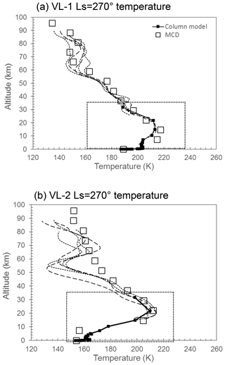
Figure 8 Fit of the column model to the soundings at $L_{\text{S}}=\mathrm{270}{}^{\circ }$ using the adjustment for adiabatic heating found in Sect. 3. For the boxes in each figure please refer to Fig. 9.

Figure 9 Comparison of the derived vertical wind speed (positive downward) from the model against the average zonal and sol-averaged vertical wind speeds from the MCD for the VL-1 and VL-2 sites at L_S 270^∘.

5 Atmospheric circulation probed with the column model

In the previous section we found good agreement between the model and the temperature soundings at the spring equinox, summer solstice and autumn equinox. The observed temperature at the winter solstice was found to be significantly warmer than the column model by up to 20 and 60 K at the VL-1 and VL-2 sites, respectively. Warming of the atmosphere by this amount has been reproduced in climate models suggesting large departures from radiative equilibrium. The warming is thought to be the heating from adiabatic compression of the atmosphere from the systematic downward motion of the air due to the seasonal meridional circulation (Heavens et al., 2011).

Figure 7 shows the location of the landing sites for VL-1, VL-2 and MSL in relation to the downwelling regions and the horizontal winds at 20 km height, which meander around Mars as planetary waves (Read and Lewis, 2004). The downwelling branch in the northern hemisphere varies in intensity longitudinally. This is due to longitudinal variations in topography and surface thermal properties. For example variations in topography tends to modify the flow concentrating it into currents, i.e. western boundary currents that flow down the flanks of Tharsis and Syrtis.

To reproduce the atmospheric heating at the latitudes of the VL-1 and VL-2 sites we can add an adiabatic heating term as described in Sect. 3 to the column model. As can be seen in Fig. 8a and b there is a significant improvement in the agreement between the model and the soundings when adding an adiabatic heating term. The fitting parameter together with the parameters for the shape of the vertical wind profile can be found in Sect. 3. By fitting the model temperature profile to the soundings, then, in principle, the vertical wind speed at each site can be estimated. However, the atmospheric temperature over each site will also be heated or cooled by horizontal advected air masses due to the strong westerlies at the VL-1 and VL-2 latitudes.

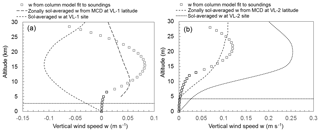
Figure 9a and b compares the resulting vertical wind profile from fitting the column model with MCD data. As indicated in Sect. 3.2 the vertical wind profile in the model is kept constant throughout the entire sol and varied after each sol to obtain a fit of the model to the sounding. This is because we are interested in influences from large-scale processes, such as horizontal advection, on the local environment. There is some diurnal variation in the vertical wind profile; going by its periodicity, we assume it to be caused by more local influences on the atmosphere.

Included on each plot is a zonally sol-averaged profile created from MCD data. These profiles were calculated as follows. For each degree of longitude the average vertical wind profile over 1 sol ($L_{\text{S}}=\mathrm{270}{}^{\circ }$) was calculated. The resulting set of profiles were then averaged to create the zonally sol-averaged profile. In addition, local (i.e. at each landing site) sol-averaged profiles are plotted. This is the vertical wind profile at the longitude and latitude of the landing site averaged over 1 sol at the winter solstice.

For the VL-1 site the maximum speed determined from the model, as shown in Fig. 9a, is 0.08 m s⁻¹ and occurs at an altitude of 16 km above the surface. The maximum vertical wind speed for the sol-averaged profile from the MCD at the VL-1 site is −0.11 m s⁻¹ and occurs at an altitude of 10 km above the surface. The directions of the vertical wind speeds do not compare well. This may not be surprising as strong westerlies at that latitude will horizontally advect heat away or into the region above VL-1, resulting in an atmospheric temperature profile that is not directly related to the local diabatic and adiabatic processes.

Figure 7 shows an intense region of downwelling air centred around a longitude of −120^∘ E from where the adiabatically generated heat could perhaps be transported to the VL-1 site by horizontal advection (Showman et al., 2013). The time taken for an air parcel travelling at 40 m s⁻¹ to cover 5400 km distance to the VL-1 site would take about 0.9 sols. This is comparable to the radiative lifetime of the Martian atmosphere of 1–2 sols.

The zonally sol-averaged temperature, that represents the region to the west of the VL-1 site, is plotted in Fig. 9a. This shows an improved agreement with the model-derived vertical wind speed. Here the maximum vertical wind velocity is 0.05 m s⁻¹ and occurs at an altitude of 10 km. However, this altitude is lower than the model-derived profile, which may be because the warm horizontally advected air is raised to a higher altitude by rising air currents as it approaches the VL-1 site.

For the VL-2 site the maximum speed determined from the model, as shown in Fig. 9b, is 0.12 m s⁻¹ and occurs at an altitude of 20 km above the surface. The maximum vertical wind speed for the sol-averaged profile from the MCD at the VL-2 site is 0.25 m s⁻¹ and occurs at an altitude of 15 km above the surface. The values for the vertical wind speeds do not compare well although the altitude and direction are in close agreement. Again horizontal advection is probable playing an important role is this region. However, VL-2 appears to be at an latitude where the vertical wind speed and direction are more consistent, presumably being less influenced by the topography that helps focus the jet streams at the latitude of VL-1 (Joshi et al., 1995). Averaging the vertical wind speed then produces quite a good agreement with the model-derived vertical wind speed.

6 Concluding remarks

We have described and demonstrated a software application that provides database query and data analysis tools for streamlining investigations of the Martian atmosphere. The main components of the software application include a column model, MCS sounding observations and a software wrapper. The software wrapper uses the Pandas data framework to allow the soundings, stored on a host machine, to be quickly accessed. Searching uses a filter with parameters set using a GUI. The column model is a 1-D model that has been extensively used to model the planetary boundary layer.

The column model was initialised with data from the soundings observations. The optical depth, tau, of the atmosphere at the time of the soundings was obtained from the MCD. Soundings were selected around the VL-1, VL-2 and MSL landing sites as these are well characterised regions of Mars.

We found that the column model usually reproduced the lapse rate and average temperature observed in vertical profiles derived from the Mars climate sounder observations. The column model was also found, in the majority of cases, to compare favourably with the Mars Climate Database. Soundings extracted by our software, spanning an area of 5–10^∘ latitude and longitude and over a range in areocentric longitude of 1–2^∘, were similar with little difference (< 5 K) in temperature between each other in temperature).

We found significant differences between the column model, which essentially represents an atmosphere in radiative equilibrium above the planetary boundary layer, and the soundings at the VL-1 and VL-2 sites but not at the MSL site during the winter solstice. We suspect heating of the atmosphere by the meridional Hadley cell circulation downwelling over the middle and high latitudes in winter was likely responsible for this mismatch.

A hill-climbing algorithm was used to vary the parameters of an adiabatic heating term added to the column model to fit it to the soundings. We found that the required maximum vertical velocity over the VL-1 site reached a maximum of 8 cm s⁻¹ at an altitude of 15 km at $L_{\text{S}}=\mathrm{270}{}^{\circ }$. At the VL-2 site, the respective maximum vertical velocity was 12 cm s⁻¹ at an altitude of 20 km. The model-derived vertical velocity profile corresponded significantly better with the zonal average of w(z) obtained from the GCM-based MCD than with w(z) obtained over the landing sites. The fitting approach developed here then provides a way to independently estimate or observe the vertical motion in the Martian atmosphere.

Future modifications to the framework will likely be the inclusion of a generalised hill-climbing algorithm. This could enable the variation of multiple parameters in the model. This would then enable us to fit temperatures from individual layers in the model to the soundings. Alternatively it could allow the variation of multiple properties, such as opacity, wind speed, etc., to find a fit between the model and the soundings.

Appendix A: MCS sounding information

Table A1 MCS sounding details, thermal inertia and albedo for the VL-1 site.

Table A2 MCS sounding details, thermal inertia and albedo for the VL-2 site.

Table A3 MCS sounding details, thermal inertia and albedo for the Curiosity site.

Appendix B: Description and examples of the working environment

The operation of the framework currently uses Anaconda, a platform that assists with package management, which includes a free and open-source version of Python. The framework runs under Windows in the cross-platform integration development environment of Spyder. Typically the framework is operated with two panels in Spyder with a code editor running in one panel and the Python console, for entering commands and displaying the output, in another.

Running the code first loads the MCS data into a Pandas pickle file. The MCS data that are stored locally, i.e. in the same folder as the Python code, are collected together and stored as a pickle file in binary format resulting in approximately 12 kB of memory per MCS profile. We found that a few gigabytes (∼ 3) of memory was required to explore the set of MCS data used in this work. The data we used covered several sols around each equinox and solstice in 1 year, which works out to around 20 sols worth of MCS data in total. The data and the framework can coexist on a standard laptop or desktop with room to spare for the addition of more data. The pickle file can be easily accessed from the Python console if the user wishes, for example, to check data for other profiles, e.g. dust, or other details of the MCS data not accessible from the GUI.

If a pickle file exists, i.e. from a previous run of the Python code, then this is used rather than creating a new pickle file as that takes some time. If necessary, i.e. more data are added, a new pickle file can be created by first deleting the old pickle file and then running the Python code, which will then recognise if the pickle file is missing and create a new one.

Once the pickle file has been assembled, the GUI is generated and displayed in the foreground. Entering a “0” into the GUI's analysis input field (see Fig. 3) performs a search of the MCS data based on the entries in the rest of the input fields. The number of profiles found using the GUI search is displayed in the Python console.

Figure B1 shows the column model with no adiabatic term (vertical wind velocity is set to zero) plotted together with a profile after a “1” has been entered into the analysis input field. Displayed next to the plots are some useful details such as the time and location of the profile. Figure B1 is a screen capture from the Python console and is what the user would see.

Figure B2 illustrates how a fitting operation would be conducted. Firstly the top image, included as a reference, shows a plot of the MCS profile and model run without the adiabatic heating term (velocity set to zero). The figure is a result of using the search parameters as indicated in the GUI in Fig. 3 and entering “1” into the analysis input field. The bottom image in Fig. B2 is a plot of the MCS profile and the column model with the adiabatic term fitted to the profile. This is a result from entering a “2” into the analysis input field. The target temperature values for the fitting algorithm can either be defined automatically, using values from the observed temperatures, or defined manually in the Python code using values from a MCD profile.

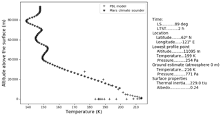
Figure B1 A visual comparison of a MCS temperature profile and a model run without the adiabatic term. This is a result of entering “1” into the analysis input field in the GUI shown in Fig. 3.

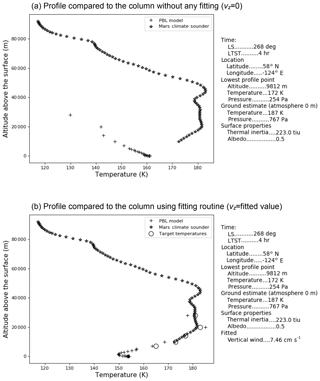
Figure B2 Fitting of the model to the MCS temperature profile using target temperatures. Panel (a) shows the results of a column model, without the adiabatic heating term, initialised based on MCS data for the particular profile shown. Panel (b) shows the results after the fitting algorithm is run. The open circles are the target temperatures for the fitting algorithm. The figure is a result of entering a “2” into the analysis field of the GUI shown in Fig. 3. Vertical wind and v_z are the maximum vertical wind speed from Eqs. (2) and (3) in Sect. 3.2.