the Creative Commons Attribution 4.0 License.
the Creative Commons Attribution 4.0 License.
 | 05 Aug 2022
Measurements of natural airflow within a Stevenson screen and its influence on air temperature and humidity records
Climate science depends upon accurate measurements of air temperature and humidity, the majority of which are still derived from sensors exposed within passively ventilated louvred Stevenson-type thermometer screens. It is well-documented that, under certain circumstances, air temperatures measured within such screens can differ significantly from “true” air temperatures measured by other methods, such as aspirated sensors. Passively ventilated screens depend upon wind motion to provide ventilation within the screen and thus airflow over the sensors contained therein. Consequently, instances of anomalous temperatures occur most often during light winds when airflow through the screen is weakest, particularly when in combination with strong or low-angle incident solar radiation. Adequate ventilation is essential for reliable and consistent measurements of both air temperature and humidity, yet very few systematic comparisons to quantify relationships between external wind speed and airflow within a thermometer screen have been made. This paper addresses that gap by summarizing the results of a 3-month field experiment in which airflow within a UK-standard Stevenson screen was measured using a sensitive sonic anemometer and comparisons made with simultaneous wind speed and direction records from the same site. The mean in-screen ventilation rate was found to be 0.2 m s−1 (median 0.18 m s−1), well below the 1 m s−1 minimum assumed in meteorological and design standard references, and only about 7 % of the scalar mean wind speed at 10 m. The implications of low in-screen ventilation on the uncertainty of air temperature and humidity measurements from Stevenson-type thermometer screens are discussed, particularly those due to the differing response times of dry- and wet-bulb temperature sensors and ambiguity in the value of the psychrometric coefficient.
- Article
(7969 KB) - Full-text XML
- BibTeX
- EndNote


Accurate measurements of air temperature and humidity require the sensors to be protected from direct or reflected solar and terrestrial radiation and precipitation. The most common exposure for such instruments remains that within a passively ventilated thermometer screen or radiation shelter, of which there are many different varieties and patterns in use worldwide: many can be broadly classed as Stevenson-type thermometer screens, otherwise known as Cotton Region Shelters in the US (Burt, 2012). These typically comprise a double-louvred enclosure, traditionally of wood painted gloss white, but increasingly consisting of UV-resistant glossy white plastic, with a double roof and base. The drawback of this type of thermometer screen (one shared by the smaller multi-plate radiation shields typically used in automatic weather stations) is that the double-louvred construction, whilst effective at reducing radiation exchange with its surroundings, also acts as a very significant barrier to natural ventilation through the body of the screen. Such reduction in airflow may result in significant and persistent departures in air temperature and humidity from “true” conditions, including excess warming of the screen interior and increases in sensor response time and extended screen lag times, especially when conditions are also changing rapidly. In addition, variations in the psychrometric coefficient at low airflow increase uncertainty in the determination of humidity parameters. Two or more of these factors often occur simultaneously and may persist for considerable periods of time, both in daylight (strong sunshine, light winds) or at night (when wind speeds tend to be lower). Implications and consequences, with examples, are subsequently considered in more detail.
It is therefore surprising that few measurements of ventilation speed have been attempted within Stevenson screens; this is perhaps because instruments combining unidirectional sensitivity to very low air flow speeds (<0.1 m s−1) are a relatively recent innovation. Limited investigations in Poland by Swioklo (1954) suggested that wind speeds inside screens amounted to about 10 % of external wind speeds, while Folland (1977) suggested 15 % of 10 m wind speeds, based upon 19 data points. A similar investigation by Bultot and Dupriez (1971) at Uccle in Belgium showed that in a large screen a ventilation rate of 1 m s−1 was reached only very exceptionally and that more often it was between 0.2 and 0.6 m s−1. More recently, Lin et al. (2001) conducted laboratory and field trials to assess the airflow efficiency of various types of thermometer screen, including Cotton Region Shelter models as well as multi-plate radiation shields. Dobre et al. (2018) attempted to model internal ventilation rates within a Stevenson screen, and suggested that airflow <0.35 m s−1 was most typical. In contrast, ISO 17714 (International Organization for Standardization, 2007) simply assumes a ventilation rate of 1 m s−1 within modern Stevenson-type screens.
This field experiment did not attempt a detailed investigation into the variation of airflow within the screen. This could probably be assessed using an array of small, high-resolution airflow sensors within the screen to obtain point measurements with which to build a high-resolution computational fluid dynamics (CFD) model; although to minimize external influences, the experiment would be best undertaken within a wind tunnel. A very large number of different measurements would be required, varying both the direction and the speed of the airflow over the screen. Some work regarding a CFD approach to model within-screen airflow has been attempted (Dobre et al., 2018).
A field experiment was chosen instead of laboratory wind tunnel tests at the outset because the objective of the research was to quantify actual ventilation rates within a typical modern thermometer screen over a representative period under normal outdoor exposure conditions. Assessing airflow around and within a screen mounted within wind tunnel would certainly permit greater control of ambient airflow, but this would be at the risk of imperfectly representing the range of conditions within an outdoor environment, including solar radiation and precipitation.
2.1 Screen airflow measurements
A sensitive Gill WindSonic anemometer was installed within a standard plastic and aluminium MetSpec Stevenson screen within the meteorological enclosure of the University of Reading Atmospheric Observatory (51.441∘ N, 0.938∘ W, 66 m a.s.l.), which is itself located in an open position in a parkland campus. The screen was free of nearby external obstructions on all sides (Fig. 1). Within the screen, the WindSonic unit was mounted with its measurement aperture horizontal, oriented accurately towards true north, and placed close to the centre of the screen interior at about 1.25 m a.g.l. (above ground level) in a position representative of the typical location of temperature and humidity sensors within such a screen in the United Kingdom (Fig. 2). The instrument was secured in place within the screen by a laboratory retort stand, itself fixed in place by cable ties to prevent any movement of the sensor during the experiment. The screen was otherwise empty to avoid any obstructions to airflow within the screen from other equipment and fittings and was kept padlocked to prevent the screen door being opened during the experimental period. Data were logged by a Campbell Scientific CR1000 logger housed externally to the screen; the sensor was sampled at 1 Hz and logged at 1 min, 5 min, and hourly intervals. Logged samples included average, minimum and maximum speeds, and vector mean directions. For most of the analysis, hourly means were found to be sufficient, although 1 and 5 min records were available and were examined where additional granularity was beneficial.

Figure 1The Reading University Atmospheric Observatory enclosure. The screen nearest to the camera housed the Gill WindSonic anemometer used in this experiment, and its screen door (shown with padlock) opens to true north. This photograph was taken on 27 May 2020. Owing to the coronavirus emergency legislation, the university campus had been closed for 2 months at this time and normal grass cutting and maintenance work had been suspended. Photograph © Stephen Burt.
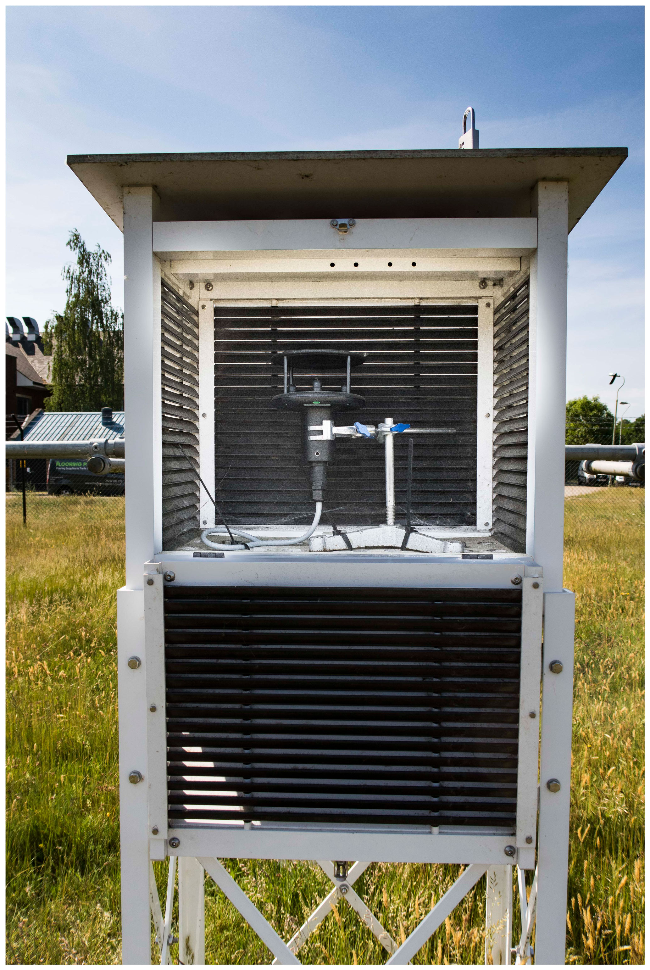
Figure 2The Gill WindSonic anemometer located within the Stevenson screen shown in Fig. 1. The inside dimensions of the screen were 50 cm width × 25 cm depth × 43 cm height. This photograph was taken on 27 May 2020. Photograph © Stephen Burt.
2.2 Calibration and uncertainty
The WindSonic unit was less than 6 months old at the outset of the measurement programme. The manufacturer's calibration uncertainty is within ± 2 % at 12 m s−1, with a resolution of 0.01 m s−1; the manufacturer's documentation attests that “the unit is designed not to require re-calibration within its lifetime”. A still-air test as set out by the manufacturer was carried out before and after the experiment to verify that no zero offset applied to the output, and both tests were negative. Following the in-screen experiment, the unit was exposed for 6 months at 3 m a.g.l. alongside another Vector Instruments A100L cup anemometer of known manufacturer calibration. Above 1 m s−1 wind speed and over a wide range of speeds, both instruments agreed within 2 % as expected. However, discontinuities resulting from the starting and stopping speed of the cup anemometer at about 0.4–0.5 m s−1 rendered a similar comparison at speeds below 1 m s−1 impractical, as a result of which there remains some uncertainty as to whether the manufacturer's ± 2 % specification is valid at the lower speed ranges found to be typical of in-screen ventilation rates. The possible impact of this uncertainty upon derived conclusions is considered in more detail in Sect. 3, but even the assumption of a much greater uncertainty (+20 %) on logged values at low speeds does not significantly affect the general conclusions of the work.
The anemometer was installed on 13 February 2020, and data were logged continuously until the unit was removed on 27 May 2020, except for 3 d record that was lost for 11–14 April. The latter was a result of the closure of the university campus due to coronavirus emergency measures. Unfortunately, data from the logger could not be retrieved before being overwritten. Access to the observatory and logger was next possible on 7 May, when all data since 14 April were successfully downloaded. In all, records from 145 433 min (2423 h, 101 d) were available for this analysis.
2.3 External wind speed and direction measurements
Routine measurements of wind speed at 2 and 10 m a.g.l., together with the wind direction at 10 m, are also made within the observatory enclosure using Vector Instruments cup anemometers calibrated in accordance with manufacturer recommendations with an expected uncertainty of ± 0.1 m s−1. These are sampled and logged every second using a Campbell Scientific CR9000X logger (along with numerous other sensors and research instruments within the meteorological enclosure). Hourly means (resolution 0.1 m s−1) were used in this analysis, with shorter time periods available for examination as required.
2.4 Rationale for the choice of differing instruments
The classical approach to an experiment of this type would suggest identical instruments be chosen for both interior and exterior measurements in order to compare like with like. However, for this experiment the Gill WindSonic sensor was consciously chosen for in-screen airflow measurements because previous pilot tests had demonstrated its ability to provide reliable measurements of wind speed at very low ventilation rates, typically well below the expected starting or stopping speeds of conventional cup anemometers. For external measurements, records from existing conventional cup anemometers at standard heights (2 and 10 m a.g.l.) were preferred precisely because of the widespread availability of similar records within meteorological data series, thus enabling the results from this experiment to be widely and directly applicable to conventional wind records made elsewhere using similar instrumentation. The external anemometers were also available and well-maintained.
The principal timescale used in this analysis is that of hourly averages; 1 min and 5 min analyses showed greater scatter, as expected, but were otherwise almost identical in pattern to hourly evaluations. During the experimental period, the distribution of wind direction was bimodal, the frequency of winds from between south-west and west approximately equalling that from winds between north-east and east (see also Sect. 3.2). Hourly mean speeds at 10 m ranged from zero to 9.6 m s−1; the maximum 3 s wind gust at 10 m was 21 m s−1, on 15 February. Aside from the abnormally high frequency of north-easterly winds during the second half of the period, wind conditions were climatologically representative of this mid-latitude inland site – the mean wind speed at 10 m during the experimental period was 2.8 m s−1, a little greater than the average for February to May (2.4 m s−1 over the preceding 5-year period) but similar to observed mean annual wind speeds.
3.1 Ventilation speeds within the screen
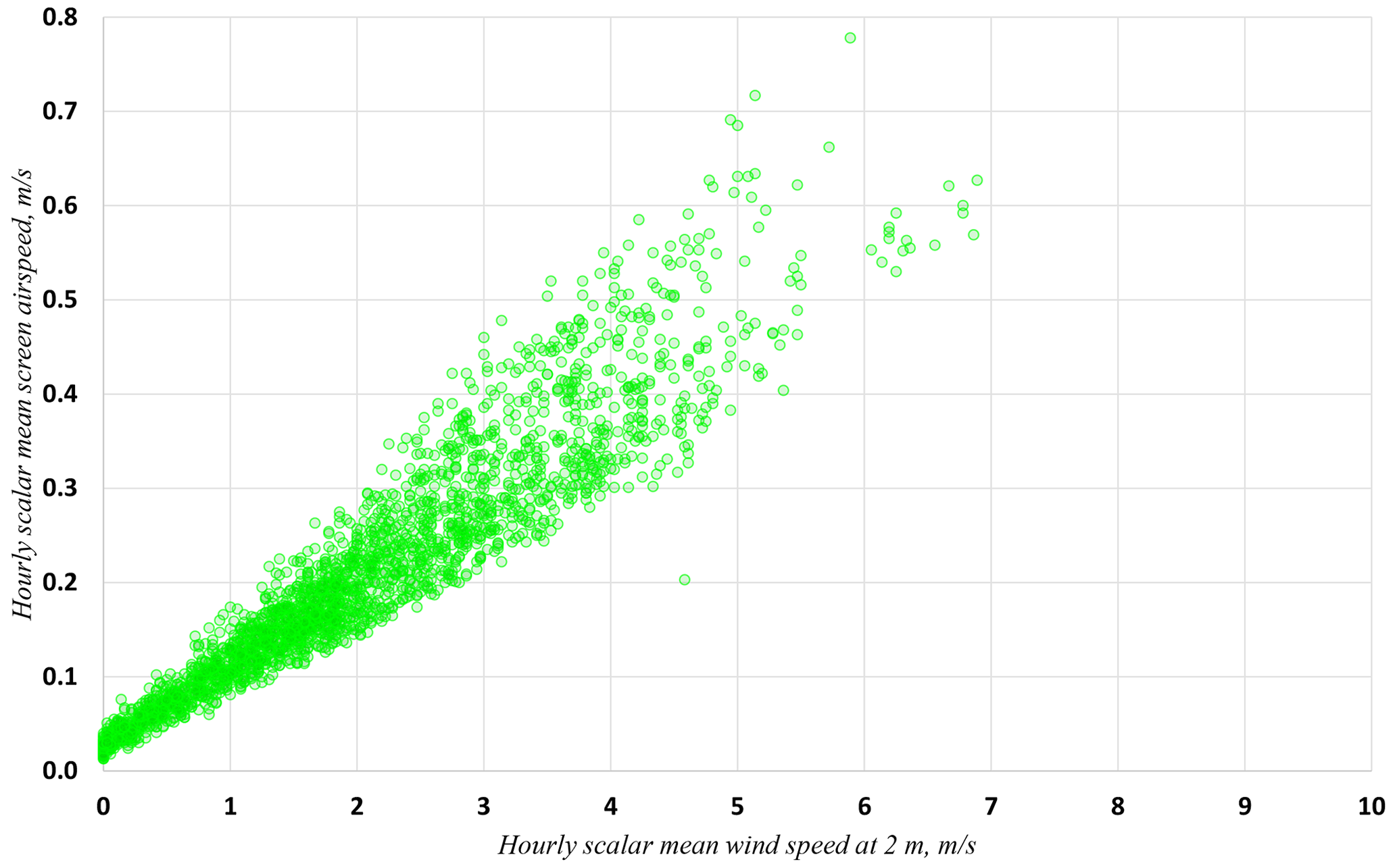
For the analysis period (13 February to 27 May 2020, excluding 11–14 April), the entire dataset consisting of 2423 h means of wind direction and speed at 2 and 10 m was used to compare external wind speed and direction with those measured using the sonic anemometer within the screen. Figure 3 shows hourly means of the in-screen ventilation speed Uscreen plotted against the simultaneous external hourly scalar mean wind speed at 10 m (U10). A very similar pattern was apparent for winds at 2 m (U2, Fig. 4), the scale differing only in reflecting the reduction in wind speed at this height. Two subsets of the data were examined in detail, as explained below.
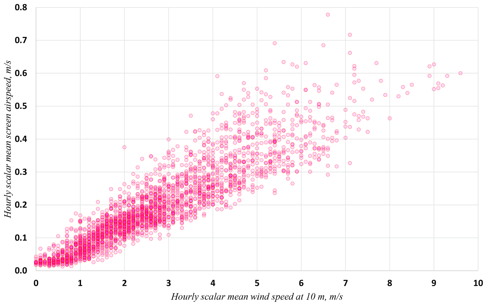
Figure 3Hourly scalar mean wind speeds within the screen (Uscreen) plotted against the external 10 m scalar mean wind speed U10 for the period 13 February to 27 May 2020. Units m s−1.
3.1.1 External wind speeds above about 1 m s−1
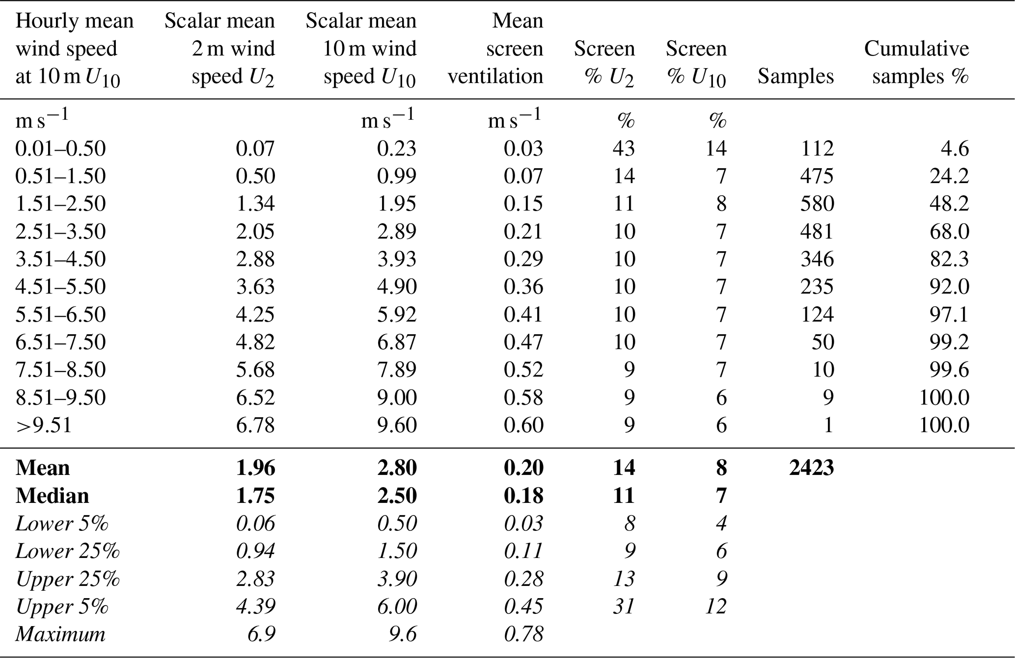
At exterior wind speeds above 1 m s−1, referencing either U2 or U10 as appropriate, screen ventilation Uscreen was close to a linear function of U10 (Fig. 3) and U2 (Fig. 4). To a near approximation when considering hourly means, Uscreen averaged just 7 % of U10 (Fig. 5) and 10 % of U2 (Fig. 6) in this subset, with the ratio decreasing slightly with increasing wind speed at both levels (Table 1). Thus, to a reasonable approximation for external wind speeds ≥ 1 m s−1, values of Uscreen for external wind measurements made at 2 m a.g.l. are given in Eq. (1), and a similar process is used for measurements at 10 m in Eq. (2):
where a total of 50 % of observations are within U2⋅ 0.10 ± 0.01, and 90 % of observations are between U2⋅0.08 and
where a total of 50 % observations are within U10⋅0.07 ± 0.01, and 90 % of observations are between U10⋅0.05 and
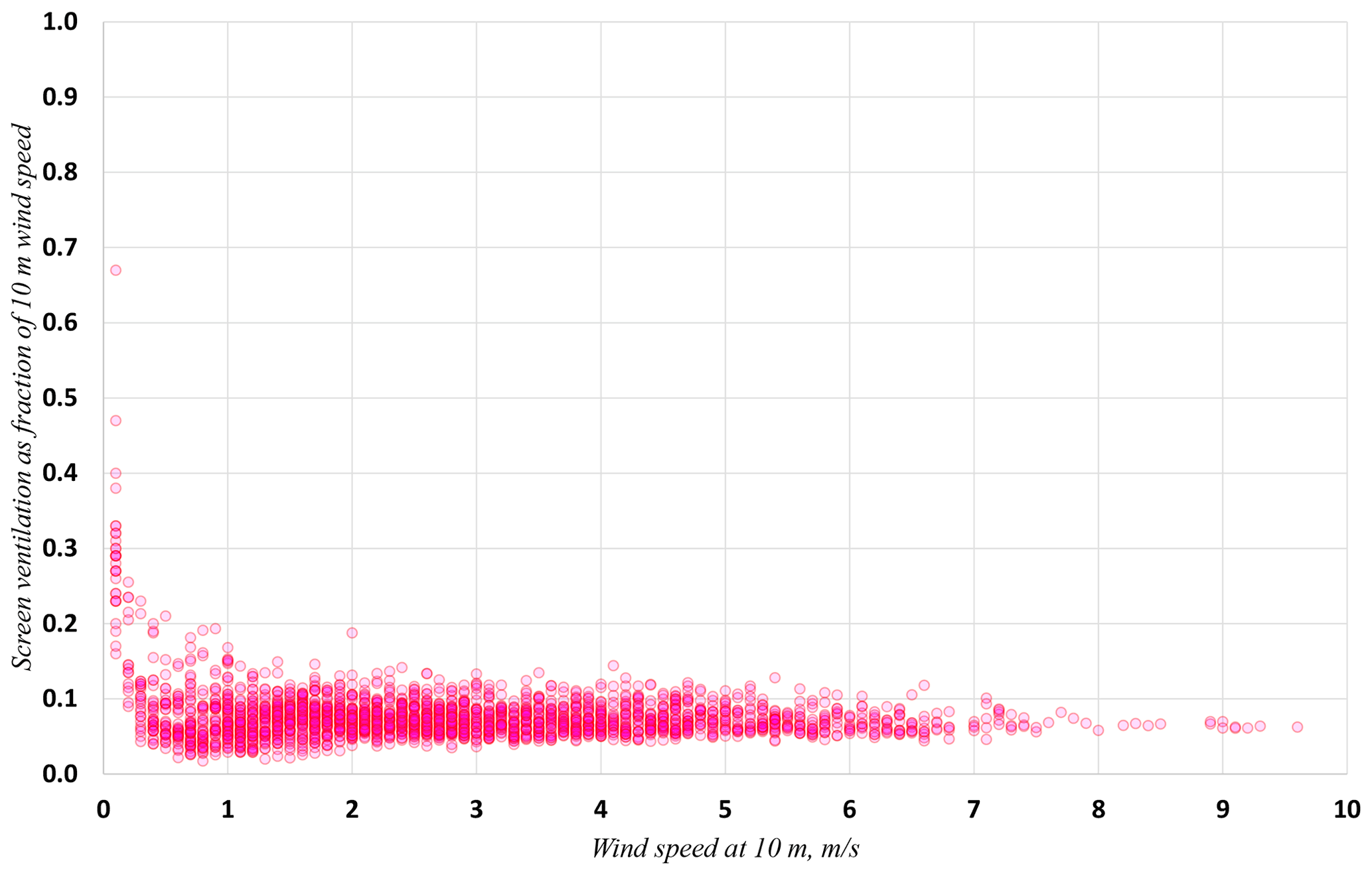
Figure 5Scatterplot of Uscreen as a fraction of U10 based on hourly scalar means. Above about 1 m s 7 % of U10.

Figure 6The same as Fig. 5 but for U2. A few values of Uscreen >U2 are omitted for clarity; see Sect. 3.1.2 for details. Above about 1 m s % of U10.
Table 1Hourly scalar mean wind speeds at 2 m and within the Stevenson screen for 1 m s−1 bins of 10 m hourly scalar mean wind speeds during the analysis period, 13 February to 27 May 2020, at the University of Reading site. Screen airflow (as % external wind speed at 2 and 10 m) excludes occasions when external wind speeds were logged as zero to avoid divide-by-zero errors. Note that the summary values include all data points; see Sect. 3.1.1 and 3.1.2 for differentiated <1 and ≥ 1 m s−1 subsets with reasoning. Means and median values are shown in bold, and other measures of statistical distribution of the entire dataset are shown in italics.
3.1.2 Light winds (external wind speeds below 1 m s−1)
In light winds, Uscreen occasionally exceeded U2 (20 h in all, around 1 % of analysis period; to avoid undue compression of the y axis these points have been omitted from Fig. 6). However, this unlikely outcome is simply explained: the sonic anemometer used for this experiment is capable of resolving wind speeds as low as 0.01 m s−1, whereas the cup anemometers used for the exterior wind records have a stopping speed of 0.4–0.5 m s−1. At low exterior wind speeds, the interior to exterior ratio therefore becomes artificially high; in reality, the ratio of Uscreen to U2 and U10 for wind speeds <1 m s−1 is probably little different to that for winds ≥ 1 m s−1.
However, the conclusions set out in the paper are insensitive to even fairly large uncertainties in the sensor's low-speed calibration, for even if the WindSonic unit's calibration at 0.2 m s−1 was in error by +20 % or 10 times the manufacturer's specification, this would result in only a minor change in the ratio of interior to exterior wind speed (from 10 % to 12 % for U2, and similarly from 7 % to 9 % for U10). While it is possible that more uncertainty attaches to the lowest speeds, this is largely irrelevant to the outcome because the typical 0.4–0.5 m s−1 stopping speed of the external U2 and U10 Vector Instruments anemometers meant that reliable comparison ratios could not be accurately obtained below these levels.
3.2 Wind direction
Although the direction of airflow within the screen is of lesser importance than its speed, comparisons were made between external hourly vector mean wind directions at 10 m and those measured within the screen by the sensitive sonic anemometer. Close correspondence with exterior wind direction was not expected, but results revealed that airflow within the screen was more complex than anticipated.
3.2.1 Wind directions at 10 m
During the experimental period, the distribution of surface winds was almost bimodal, with winds from between south-west and west and those from between north-east and east occurring with approximately equal frequency. Winds from a westerly quarter dominated the first half of the experimental period, and those from north or east dominated the second half. The wind rose in Fig. 7a shows the frequency, by 10∘ sectors and within six wind speed bins, of hourly vector mean wind directions at 10 m above ground during the experimental period; calms (here taken as hourly scalar mean wind speeds at 10 m below 0.25 m s−1) amounted to 2.3 %. The outer scale ring represents 10 % of all observations.
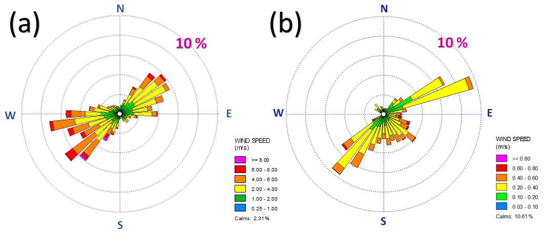
Figure 7Hourly vector mean wind direction frequencies, in wind rose format, during the experimental period: (a) at 10 m and (b) within the Stevenson screen. The outer scale ring represents 10 % frequency for both plots, but the scales and class boundaries necessarily differ. Mean wind speed was 2.8 m s−1 at 10 m and 0.20 m s−1 within the screen.
3.2.2 In-screen airflow directions
Figure 7b shows the distribution of hourly vector mean wind directions within the screen over the same period, and in the same format, as the external wind directions in Fig. 7a. To enable comparison, the scale in Fig. 7b has been expanded such that each speed division is of the equivalent exterior speed. Using this classification, “calm” (<0.025 m s−1) represents 10.6 % of all events (using the same maximum threshold as exterior wind directions, i.e. 0.25 m s−1, the figure would be 68.3 %). The outer scale ring again represents 10 % of all 2423 h records.
4.1 Wind speed
It was surprising to discover that airflow within the screen is very much less than has been conventionally assumed. ISO 17714 (International Organization for Standardization, 2007), for example, assumes a ventilation rate of 1 m s−1 within modern passively ventilated Stevenson-type screens, whereas the results presented here demonstrate that the mean ventilation within the screen during the experimental period was only 0.2 m s−1 at this fairly typical well-exposed mid-latitude inland site. In-screen airflow reached 1 m s−1 only when the external 10 m wind speed was close to 10 m s−1. Further, using 1 min mean data, an average of 1 m s−1 or more was attained for just 17 min (0.01 %) during the 101 d experimental period. Figure 8 shows the distribution of the 2423 h means of Uscreen. Perhaps surprisingly, only 110 min averaged 0.00 m s−1 airspeed within the screen, less than 0.1 % of the dataset, while the lowest hourly mean was just above 0.01 m s−1.
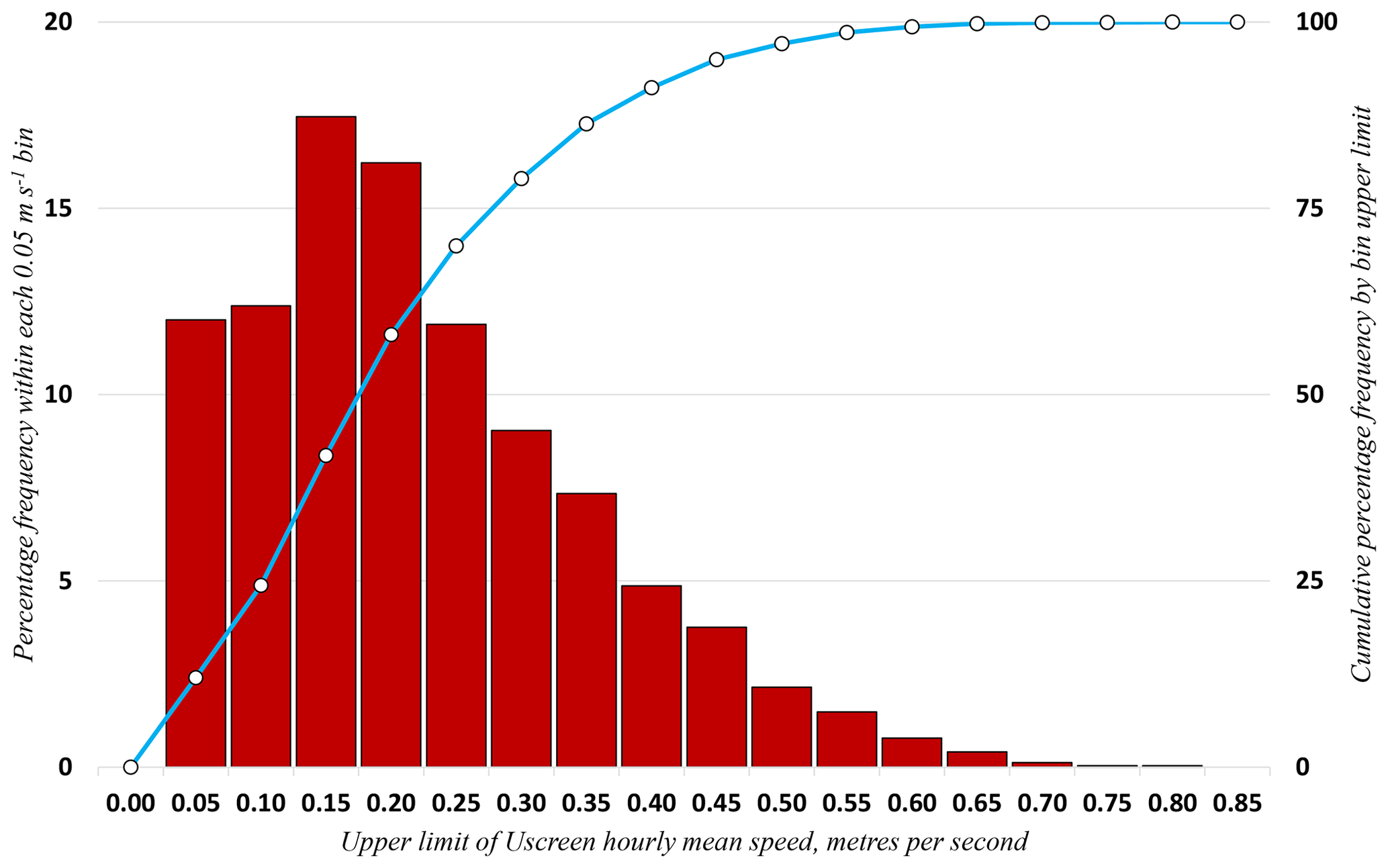
Figure 8Percentage frequency distribution of hourly mean screen ventilation Uscreen within 0.05 m s−1 bins. The red columns show per-bin frequency (left vertical axis), and the blue line and markers show the cumulative percentage frequency below upper bin limit (right vertical axis). There is a total of 2423 observations, with an hourly mean speed of 0.20 m s−1, a median of 0.18 m s−1, a minimum of 0.01 m s−1, and a maximum of 0.78 m s−1.
Whilst it would be unrealistic to assume that the relationships found in this experiment apply rigidly to all Stevenson-type thermometer screens in any climate, it is clear that an automatic assumption of 1 m s−1 internal airflow in such screens is difficult to justify, except perhaps at especially exposed sites where 10 m wind speeds frequently exceed 10 m s−1. The low mean airflow rates shown by this experiment have considerable implications for air temperature and humidity measurements, and these are discussed subsequently.
4.2 Wind direction
There is a striking difference between “external” and “internal” wind roses (Fig. 7a, b respectively). There is a suggestion here of preferential flow orientations within the screen structure itself, but a more detailed investigation would require additional sensors within the screen to provide a three-dimensional capability. Such an experiment would certainly benefit from a more controlled environment, such as a wind tunnel. However, this experiment found no evidence that the pillars of the screen structure provided any greater obstruction to wind flow from those directions (north-east, south-east, etc.) than winds orthogonal to one of the screen faces. Despite the low mean speeds, the airflow within the screen appeared to be highly turbulent in nature.
4.3 Implications resulting from low screen ventilation
The results presented have important, albeit unavoidable, implications for all measurements of air temperature and humidity taken within Stevenson-type thermometer screens where external wind speeds are typically less than 10 m s−1. There are four main effects, and it is helpful to think of these as falling into two main categories, with combinations more likely than not. The first category is where effects are primarily due to low wind speeds per se, including excess warming of the screen structure and lengthening of the screen lag time. The second relates to increasing response times of sensors within the screen and changes in the psychrometric coefficient due to decreasing airflow, both being of course themselves a consequence of low external wind speeds. Each is considered briefly in turn.
4.3.1 Excess warming of the screen interior
It is well known that certain combinations of light winds with strong solar radiation, or low-level direct sunshine on the screen exterior, can result in excess warming of the screen exterior, which by radiative exchange warms the screen interior. This tendency has been known for well over a century (Gaster, 1882; Aitken, 1884) and has been reported in numerous screen comparison trials since (see, for example, Sparks, 1972; Andersson and Mattison, 1991; Clark et al., 2014, and references therein; and Harrison and Burt, 2021). Such previous and ongoing work indicates that the magnitude of the warming is not infrequently 0.5 K and occasionally amounts to 2–3 K. The primary cause of the positive departure from “true” air temperatures is the reduced effectiveness as a result of low wind speeds of turbulent advective cooling of a screen structure heated by solar radiation. Limited in-screen airflow, itself obviously another consequence of low external wind speeds, then results in further reductions in turbulent advective heat transport within the body of the screen, as a result of which screen temperatures rise above true air temperature. Such warming persists for as long as the causative conditions (incident solar radiation and/or light winds) remain in place.
4.3.2 Lengthening of the screen lag time
Any artificial structure housing thermometers itself has a response time. The importance of ventilation rate around and within thermometer screens was examined by Harrison (2010, 2011), who found that low levels of natural ventilation led to long (5–20 min) lags in temperatures measured within a Stevenson screen. These effects were found to be both more common and more pronounced at night, when wind speeds are usually lower than during daytime, and have a proportionally greater effect on minimum rather than maximum temperatures (Harrison and Burt, 2020).
4.3.3 Increased response times of sensors within the screen
Burt and de Podesta (2020) examined the response times of a selection of typical meteorological platinum resistance thermometers (PRTs), and found their 63 % response time τ63 (s) depended primarily on sensor diameter d (mm) and ventilation speed v (m s−1). τ63 could be approximately expressed as Eq. (3) (Eq. 11 in Burt and de Podesta, 2020):
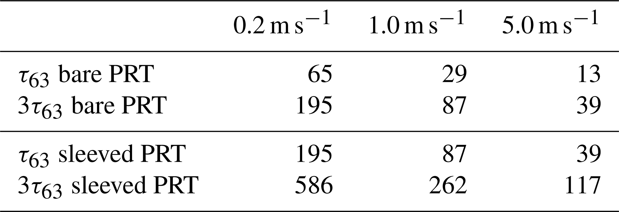
Assuming this relationship, the first row of Table 2 presents calculated τ63 response times for a nominal “bare” PRT of 3 mm diameter at various ventilation speeds, namely 0.2 m s−1 (representing the average in-screen airflow found during this experiment), 1.0 m s−1 (in-screen airflow assumed by ISO 17714, but found to occur during just 0.01 % of the entire experimental period), and 5.0 m s−1 (the airflow typical of an aspirated sensor). A bare PRT is one without sleeving around the outer steel sheath and is typical of those used in meteorological screens as a dry-bulb thermometer (Tdry) to measure “air temperature”. The second row of Table 2 is 3τ63, the time required for that sensor to show 95 % of a step change in temperature (Brock and Richardson, 2001). A 3 mm diameter PRT in a thermometer screen ventilated at 0.2 m s−1, the average level found in this experiment, will take about 195 s to respond to 95 % of a change in temperature, 5 times as long as the 39 s for an identical sensor exposed in an aspirated screen subject to 5 m s−1 airflow. The guideline in the World Meteorological Organization CIMO guide (WMO, 2018) is that a 95 % response should happen within 60 s. Without wholly unrealistic assumptions of external wind speed, some alternative method of increasing airflow across the PRT within the screen, or decreasing the diameter to the PRT to 1.5 mm or less, it would appear unlikely that this WMO guideline response time could ever be attained within a typical Stevenson screen (except in strong winds).
Table 2Comparison of calculated response times (s) for a nominal “bare” PRT of 3 mm diameter in varying airflow, and for the same sensor sleeved in a (dry) wick – here representing two identical sensors where the response time differences are due solely to the presence of the wick around the sensor. Based upon experimental work and empirical relationships described in Burt and de Podesta (2020).
4.3.4 The specific case of the wet-bulb PRT response time
A wet-bulb thermometer (Twet) is frequently used as part of a psychrometer to derive various humidity parameters, including dew point, and in operation typically comprises a PRT sleeved in a cotton wick, with the latter being kept wet by capillary action from an adjacent reservoir of distilled water (see, for example, Meteorological Office, 1981b; or Harrison, 2014). However, the cotton wick also acts to insulate and dampen the response of the PRT to changes in temperature: informal experiments suggest that the response time of a dry “sleeved” PRT at 1.0 m s−1 airflow increases by about a factor of 3 at room temperature (experimental results ranging from 2.5 to 3.7; see also Table V in Meteorological Office, 1981b). It is non-trivial to design an effective response time experiment with a wetted wick because the resulting temperature response is complicated by evaporation, latent heat, the different specific heat capacities of water and sensor materials, and conduction through the wick. Rows 3 and 4 in Table 2 show the indicative impact upon response times of an identical sensor sleeved within a cotton wick of the type commonly used for wet-bulbs. Following the same logic as above, it can be seen that within a screen ventilated at 0.2 m s−1, a typical wet-bulb response time to 95 % of a change lies little short of 10 min. Even a continuously aspirated wet-bulb – if such a device could be developed to be both practically and operationally feasible – would take almost 2 min to attain 95 % response for a 3 mm sensor, although an aspirated wet-bulb PRT 1.5 mm in diameter or less could theoretically do so in about 64 s. An Assmann psychrometer (see, for example, Foken, 2022) includes both aspirated dry- and wet-bulb thermometers, but for several reasons (particularly the difficulty in arranging for a constant and reliable supply of water to the wet-bulb wick in all conditions, and in maintaining a clean wet-bulb surface) it is unsuited to continuous automatic operation.
The very different response times of bare and sleeved PRTs illustrate a further issue pertaining to wet-bulb temperatures (and humidity parameters derived therefrom) following rapid changes in air temperatures. Figure 9 illustrates a hypothetical case setting out the cooling curve of two 3 mm PRTs, one a bare dry-bulb (solid line) and one “dry but sleeved” PRT (dashed line), in response to an instantaneous reduction in dry-bulb temperature from 20 to 15 ∘C, assuming 0.2 m s−1 airflow. This is a deliberately simplified scenario ignoring latent heat effects; the intention here is to demonstrate the impacts of differing response times rather than to suggest a realistic model of a physical wet-bulb sensor. The τ63 response times of the two sensors are 65 and 195 s, as given in Table 2, the sleeved sensor being much slower than the unsleeved sensor owing to the insulating properties of the sleeve material. Let us further assume that the relative humidity (% RH) at t=0 is 85 % (for which the wet-bulb temperature at t=0 would be 18.5 ∘C), that the ambient % RH remains constant at 85 throughout the change in temperature, and that the response time of the second PRT matches that of an actual wet-bulb. Then it can be seen from Fig. 9 that the slower cooling of the sleeved PRT results in a sudden but spurious increase in % RH (dotted line, right-hand vertical axis); from about t=40 s for over 200 s the calculated % RH exceeds 100 (in which circumstance, by convention, the result is capped at 100 %). The true % RH does not return to the nominal unchanged 85 until after about t=1000 s (about 17 min) following the nominal drop in temperature. The dew point (dashed grey line in Fig. 9) actually increases until t≈30 s, and shortly afterwards follows the dry-bulb curve during the period of nominal % RH = 100.
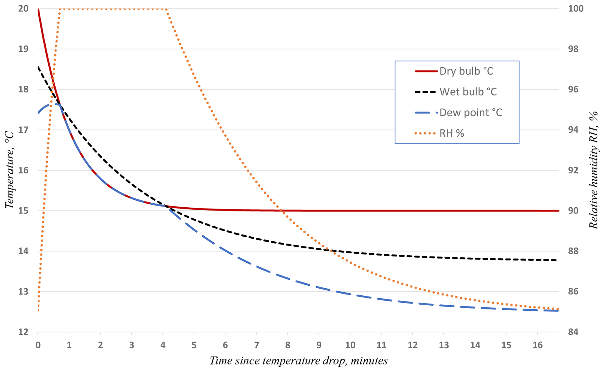
Figure 9Time series (min) of dry-bulb, nominal wet-bulb, and calculated dew point temperatures (∘C, left axis) and relative humidity (% RH, right axis) following an instantaneous fall in temperature of 5 K from 20 ∘C, assuming sensor response times per Table 2.
Events such as those outlined above do occur occasionally in the real world, but their transitory nature implies that manual observations of instances of “wet-bulb thermometer higher than dry-bulb” would be infrequent, even at sites where hourly observations were made. Given such circumstances, it would not be surprising if the observer simply ascribed an anomalous “high” wet-bulb reading to instrumental error, for minor differences – say within 0.2 K, particularly at high % RH – could be expected to lie within instrumental calibration tolerance. The most likely outcome would be that a wet-bulb reading no higher than the dry-bulb would be entered. If the wet-bulb reading was entered as higher than the dry-bulb reading, it is likely that a similar correction would ensue in subsequent dataset quality control processes. However, such events can be expected to be more obvious where higher temporal resolution is available from automatic weather station datasets, and provided instrumental calibrations are accurately known, they should not necessarily be assumed to be incorrect but may simply reflect differing sensor response times.
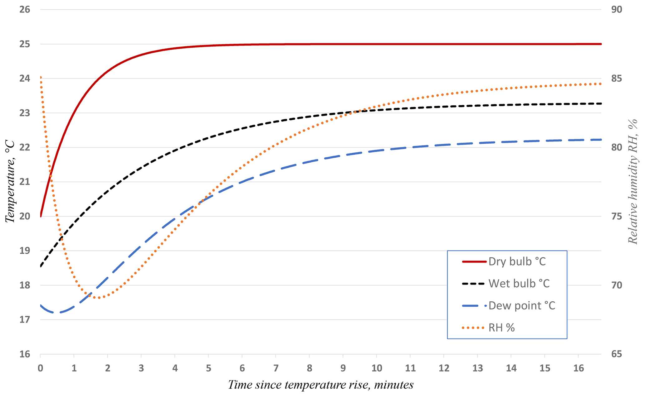
The example of a nominal instantaneous increase in air temperatures, less common in meteorological situations, of similar magnitude is illustrated in Fig. 10. Here the calculated % RH falls rapidly to below 70 around t=100 s and does not recover to the nominal 85 until about t=780 s (13 min).
The known sources of error when measuring humidity using dry- and wet-bulb psychrometers provide the opportunity at this point to refer to the advantages of electronic relative humidity sensors – which include faster response times (except at high % RH), reduced maintenance requirements, a lack of dependency upon a water supply, reliable operation below 0 ∘C, and simplified logger algorithms. For more details the reader is referred to, for example, Burt (2012) and Harrison (2014).
4.3.5 Implications for sensor averaging time
The WMO CIMO guide (WMO, 2018, Annex 1A) recommends a 60 s averaging time for both temperature and humidity sensors. Whilst this is a reasonable statement of requirement, from the above discussion it can be seen that 95 % response times (3τ63) of even the fastest commercially available Pt100 sensors can be expected to be substantially in excess of this when exposed within passively ventilated Stevenson screens and longer still when configured as a wet-bulb (i.e. sleeved with a cotton wick). Table 3 illustrates the resulting errors in 1 min means from 1 to 10 min following the previous example in Fig. 9 of an instantaneous 5 K fall in temperature (and constant 85 % RH) at t=0 s, assuming response times that are given in Table 2. It should be noted that the response times set out in Table 2 are representative of the fastest commercial Pt100 sensors available in 2020 (Burt and de Podesta, 2020) and that the response times of typical Pt100 sensors are almost certainly slower still.
Table 3Tabulated 60 s running mean values for each minute (the average of the preceding 6×10 s sampled values) following an instantaneous reduction in dry-bulb temperature from 20 to 15 ∘C at t=0 and a nominal wet-bulb temperature, assuming response times as for the dry- and wet-bulb thermometers in Table 2. All values are given to one decimal place. Note that the nominal wet-bulb temperature is above the dry-bulb temperature until after t=4 min.
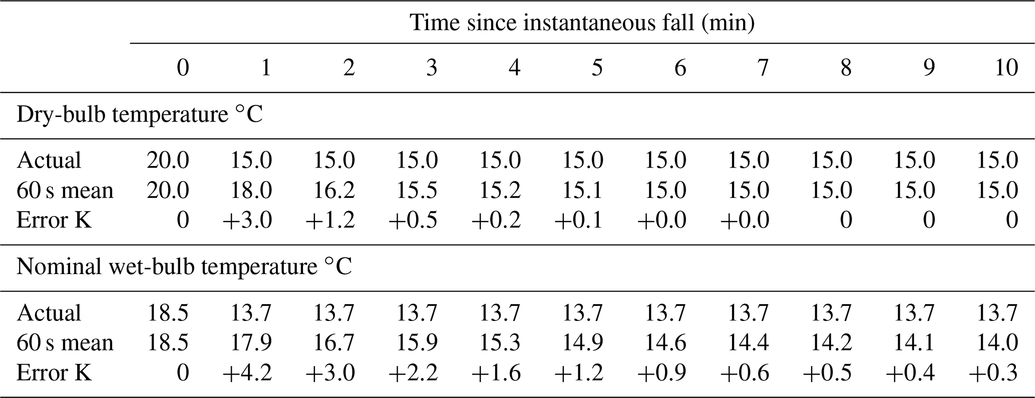
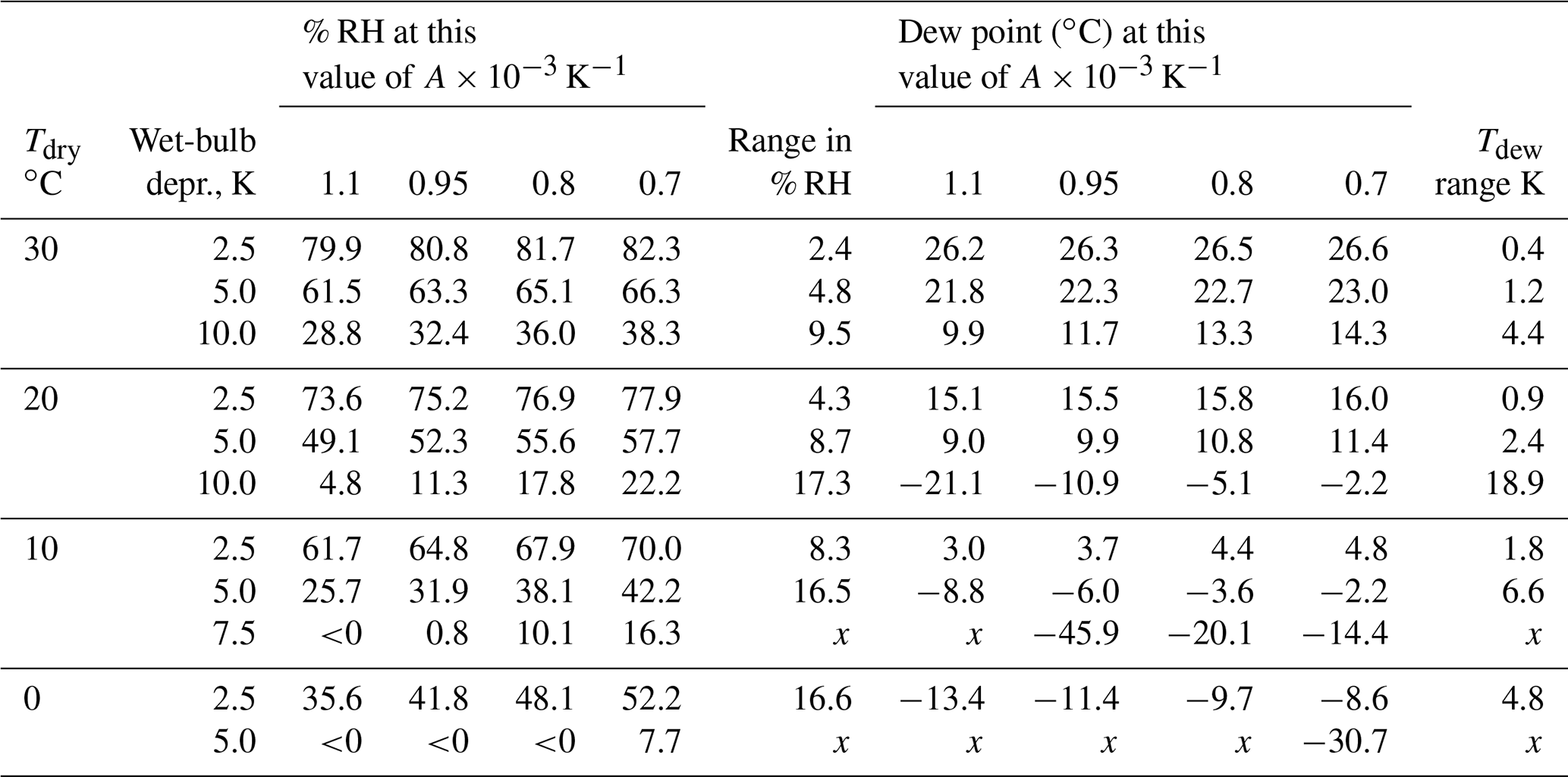
Table 4Values of % RH and dew point (∘C), and the range in values, calculated for various values of the psychrometric coefficient A ( K−1), for a selection of values of dry-bulb temperature (Tdry, ∘C) and wet-bulb depression (K). Parameter combinations producing % RH below zero, for which the dew point is undefined (x), are indicated as <0.
4.3.6 Variations of psychrometric coefficient at low airflow
The efficiency of the wet-bulb and the assumptions used in the psychrometric equation to derive atmospheric humidity parameters from the readings of a dry- and wet-bulb psychrometer vary significantly with ventilation speed. A value of % RH can be determined by first calculating the vapour pressure e (in hPa) from Eq. (4):
and then calculating % RH from Eq. (5):
where A is the psychrometer coefficient ( K−1), p is the atmospheric pressure (in hPa/1000), and es(T) is the saturation vapour pressure of water at temperature T ∘C, Tdry ∘C or Twet ∘C, as context applies.
Harrison and Wood (2012) showed that the value of the psychrometric coefficient A increases steeply from K−1 in airflow ≥ 1 m s−1 to between 0.8 and 1.2–1.3 K−1 below 0.5 m s−1. The key point here is that screen ventilation has been shown to almost always be below 0.5 m s−1 (>99 % below 0.5 m s−1, Table 1), and thus A lies in a region where variation with ventilation speed is considerable. This is shown graphically in Fig. 11, which has been adapted from Fig. 6.18 of Harrison (2014) by adding a shaded box showing the 5 % and 95 % percentiles of the screen ventilation results described here.
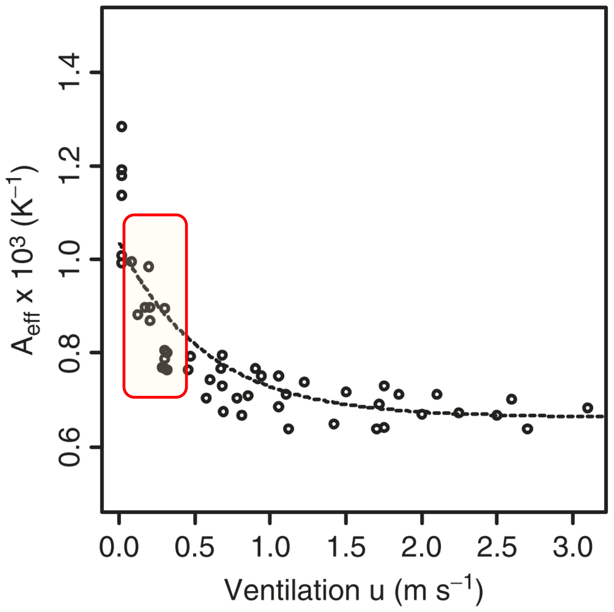
Figure 11Dependence of the psychrometer coefficient A on ventilation speed. Figure is adapted from Fig. 6.18 of Harrison (2014). The shaded box overlay shows the 5 % and 95 % percentile limits of screen airflow observed during this experiment.
To illustrate the possible range of uncertainty, Table 4 sets out calculations of % RH and dew point for several combinations of dry-bulb temperatures and wet-bulb depressions, with A varying between 0.7 and K−1, corresponding approximately to the 5 %–95 % range of observed in-screen airflow velocities. The calculation method for relative humidity and dew point from dry- and wet-bulb temperatures follows that set out in Harrison (2014). The values set out in the table are as follows:
-
A=1.1 ( K−1), assuming a ventilation speed close to zero;
-
A=0.95, the observed 0.2 m s−1 mean value of in-screen airflow found in this experiment;
-
A=0.8, airflow at about 0.5 m s−1, such as might be expected in a Stevenson screen of the type tested with U10≥ 7–8 m s−1 approximately, from Table 1;
-
A=0.7, airflow at ≥ 1 m s−1, such as could be expected from an aspirated dry- and wet-bulb psychrometer, such as an Assmann psychrometer, and the in-screen ventilation level assumed in ISO 17714.
It should be kept in mind that increased airflow across the sensors would also result in significant improvements in response time. Even at moderate values of air temperature and wet-bulb depression, and necessarily assuming zero rate of change of either temperature, differences between the assumption of ≥ 1.0 m s−1 airflow ( K−1, ISO 17714 assumption, or aspirated sensors) and 0.2 m s−1 ( K−1, mean in-screen airflow found in this experiment) are at least as great as those resulting from 0.1 K calibration uncertainty in either temperature. For example, at Tdry 10 ∘C and Twet 7.5 ∘C, the range in % RH applicable to 0.2 m s−1 or 1.0 m s−1 ventilation is from 64.8 % to 70.0 % and dew point from 3.7 to 4.8 ∘C; a ± 0.1 K change in dry-bulb temperature would vary % RH by only ± 2 %–3 % and dew point by ± 0.3 K at such temperatures. The range of variation increases sharply with lower airflow, lower temperatures, and greater wet-bulb depressions, such that the combination of Tdry 10 ∘C and Twet 2.5 ∘C generates an unrealistic % RH below zero and undefined dew point with K−1 (for a near-zero airflow), in contrast to K−1 (for a 1 m s−1 airflow), which produces a more realistic % RH = 16 and dew point −14.4 ∘C.
Climate science depends upon accurate measurements of air temperature and humidity, and ventilation speeds within Stevenson-type thermometer screens have important implications for the accuracy and reliability of such measurements. In-screen airflow significantly impacts the response times of sensors within the screen and affects how representative conditions within the screen are of external air temperature and humidity – especially in conditions of strong solar radiation and/or light winds. This experiment has shown that current assumptions of ventilation speeds within Stevenson screens are too optimistic; the ISO 17714 assumption of 1 m s−1 airflow (International Organization for Standardization, 2007) was attained for only 0.01 % of the 3-month experimental period. Of course, the results set out here refer only to a single pattern of screen sited inland within a relatively sheltered temperate-latitude wind climate for a period of little more than 3 months. However, the consistency of the results in a representative wind climate and under typical enclosure and exposure conditions suggests wider applicability. That is not to suggest that every measurement of temperature or humidity made within Stevenson screens should be disregarded or retrospectively corrected, even if that were feasible. Instead, based upon sound physical and metrological principles, we should define what is meant by true air temperature (and humidity) and then accelerate the development, piloting and deployment of standardized alternative methods and practices to measure these elements with reduced uncertainty. In doing so, we should of course also take care to provide periods of overlap with existing methods to minimize future data homogeneity issues, particularly for long-period sites. The Stevenson screen will likely be with us for some time to come.
The complete experimental results are available on Figshare, https://doi.org/10.6084/m9.figshare.19889515.v1 (Burt, 2022) as a single Excel file containing two worksheets, the first sheet describes the file format, and the second sheet contains the entire hourly dataset.
The author has declared that there are no competing interests.
Publisher's note: Copernicus Publications remains neutral with regard to jurisdictional claims in published maps and institutional affiliations.
Thanks go to my University of Reading colleague Giles Harrison for helpful support and suggestions prior to and during the experiment and to Ian Read from the Technical Services team for assistance with experimental arrangements and setup. I am also very grateful for the helpful and constructive comments from the referees that improved this paper.
This paper was edited by Andrew Wickert and reviewed by Mike Molyneux, S. Bell, and one anonymous referee.
Aitken, J.: Thermometer Screens, P. Roy. Soc. Edinb., 12, 661–696, 1884.
Andersson, T. and Mattison, I.: A field test of thermometer screens, SMHI Report No. RMK 62, Norrkoping, Sweden, https://www.smhi.se/polopoly_fs/1.148394!/RMK_62.pdf (last access: 24 July 2022), 1991.
Brock, F. V. and Richardson, S. J.: Meteorological Measurement Systems, chapt. 6, Oxford University Press Oxford, 290 pp., https://doi.org/10.1093/oso/9780195134513.001.0001, 2001.
Bultot, F. and Dupriez, G. L.: Comparaison d'instruments de mesure de l'humidité de l'air sous abri (Comparison of humidity measuring instruments in(side) a shelter), Arch. Meterol. Geophys. Bioklimatol. Wien, 19B, 53–67, 1971.
Burt, S.: The Weather Observer's Handbook, chap. 5, Cambridge University Press, New York, 444 pp., https://doi.org/10.1017/CBO9781139152167, 2012.
Burt, S. and M. de Podesta: Response times of meteorological air temperature sensors, Q. J. Roy. Meteorol. Soc., 146, 2789–2800, https://doi.org/10.1002/qj.3817, 2020.
Burt, S.: Data files from measurements of natural airflow within a Stevenson screen, submitted to Geoscientific Instrumentation (EGU), Excel format, figshare [data set], https://doi.org/10.6084/m9.figshare.19889515.v1, 2022.
Clark, M. R., Lee, D. S., and Legg, T. P.: A comparison of screen temperature as measured by two Met Office observing systems, Int. J. Climatol., 34, 2269–2277, https://doi.org/10.1002/joc.3836, 2014.
Dobre, M., Sestan, D., and Merlone, A.: Air temperature measurement uncertainty associated to a mounting configuration temperature sensor-radiation shield, in: WMO TECO conference, Amsterdam, October 2018, https://www.wmocimo.net/wp-content/uploads/ (last access: 24 July 2022), 2018.
Foken, T. (Ed.) Springer Handbook of Atmospheric Measurements, chap. 8, Springer International Publishing, 1748 pp., https://doi.org/10.1007/978-3-030-52171-4, 2022.
Folland, C. K.: The psychrometer coefficient of the wet-bulb thermometer used in the Meteorological Office large thermometer screen, Bracknell, Meteorological Office, Scientific Paper No. 38, https://digital.nmla.metoffice.gov.uk (last access: 24 July 2022), 1977.
Gaster, F.: Report on experiments made at Strathfield Turgiss in 1869 with stands or screens of various patterns, devised and employed for the exposing of thermometers, in order to determine the temperature of the air, Meteorological Office Quarterly Weather Report, Addendum for 1879 (dated May 1880, published 1882), National Meteorological Library, Exeter, UK, 1882.
Harrison, R. G.: Natural ventilation effects on temperatures within Stevenson screens, Q. J. Roy. Meteor. Soc., 136, 253–259, https://doi.org/10.1002/qj.537, 2010.
Harrison, R. G.: Lag-time effects on a naturally ventilated large thermometer screen, Q. J. Roy. Meteor. Soc., 137, 402–408, https://doi.org/10.1002/qj.745, 2011.
Harrison, R. G.: Meteorological measurements and instrumentation, chapt. 6, in: Advancing weather and climate science, Wiley, https://doi.org/10.1002/9781118745793, 2014.
Harrison, R. G. and Burt, S.: Shall I compare thee to a summer's day? Art thou more temperate? …Sometimes too hot the eye of heaven shines …, Weather, 75, 172–174, https://doi.org/10.1002/wea.3662, 2020.
Harrison, R. G. and Burt, S. D.: Air temperature uncertainties from naturally ventilated thermometer screen measurements, Environ. Res. Lett., 3, 061005, https://doi.org/10.1088/2515-7620/ac0d0b, 2021.
Harrison, R. G. and Wood, C. R.: Ventilation effects on humidity measurements in thermometer screens, Q. J. Roy. Meteor. Soc., 138, 1114–1120, https://doi.org/10.1002/qj.985, 2012.
International Organization for Standardization (ISO): ISO 17714 Meteorology – Air temperature measurements – Test methods for comparing the performance of thermometer shields/screens and defining important characteristics, Geneva, https://www.iso.org/standard/31498.html (last access: 24 July 2022), 2007.
Lin, X., Hubbard, K. G., and Meyer, G. E.: Airflow characteristics of commonly used temperature radiation shields, J. Atmos. Ocean. Tech., 18, 329–339, 2001.
Meteorological Office: Handbook of Meteorological Instruments: Volume 2, Measurement of temperature, Second edn., London: Her Majesty's Stationery Office, ISBN 0114003246, 1981a.
Meteorological Office: Handbook of Meteorological Instruments: Volume 3, Measurement of humidity, Second edn., London: Her Majesty's Stationery Office, ISBN 0114003254, 1981b.
Sparks, W. R.: The effect of thermometer screen design on the observed temperature, World Meteorological Organization, Geneva, Publication No. 315, https://library.wmo.int/doc_num.php?explnum_id=8131 (last access: 24 July 2022), 1972.
Swioklo, Z.: The relationship of the windspeed inside a meteorological screen to the speed given by a windvane at the standard height, Warsaw, B. Serv. Hydr. Met., 3, 291–296, 1954 (in Polish; English translation in National Meteorological Library, Exeter, UK).
WMO (World Meteorological Organization): WMO No. 8 – Guide to Meteorological Instruments and Methods of Observation (CIMO guide), 2018 edn., – Volume I: Measurement of Meteorological Variables, ISBN 978-92-63-10008-5, 2018.