the Creative Commons Attribution 4.0 License.
the Creative Commons Attribution 4.0 License.
 | 13 Jun 2024
Accuracy of the scalar magnetometer aboard ESA's JUICE mission
Christoph Amtmann
Andreas Pollinger
Michaela Ellmeier
Michele Dougherty
Patrick Brown
Roland Lammegger
Alexander Betzler
Martín Agú
Christian Hagen
Irmgard Jernej
Josef Wilfinger
Richard Baughen
Alex Strickland
Werner Magnes
This paper discusses the accuracy of the scalar Coupled Dark State Magnetometer on board the Jupiter Icy Moons Explorer (JUICE) mission of the European Space Agency (ESA). The scalar magnetometer, referred to as MAGSCA, is part of the J-MAG instrument.
MAGSCA is an optical omnidirectional scalar magnetometer based on coherent population trapping, a quantum interference effect, within the hyperfine manifold of the 87Rb D1 line. The measurement principle is only based on natural constants; therefore, it is in principle drift-free, and no calibration is required. However, the technical realisation can influence the measurement accuracy. The most dominating effects are heading characteristics, which are deviations of the magnetic field strength measurements from the ambient magnetic field strength. These deviations are a function of the angle between the sensor axis and the magnetic field vector and are an intrinsic physical property of the measurement principle of the magnetometer.
The verification of the accuracy of the instrument is required to ensure its compliance with the performance requirement of 0.2 nT (1σ) with a data rate of 1 Hz. The verification is carried out with four dedicated sensor orientations in a Merritt coil system, which is located in the geomagnetic Conrad Observatory (COBS). The coil system is used to compensate the Earth's magnetic field and to apply appropriate test fields to the sensor.
This paper presents a novel method to separate the heading characteristics of the instrument from residual (offset) fields within the coil system by fitting a mathematical model to the measured data and by the successful verification of the MAGSCA performance requirement.
- Article
(5411 KB) - Full-text XML
- BibTeX
- EndNote


The Jupiter Icy Moons Explorer (JUICE) mission of the European Space Agency (ESA) aims to explore the Jovian system and its icy Galilean moons, Ganymede, Callisto, and Europa, in terms of their potentially habitable environments (Grasset et al., 2013; Hussmann et al., 2014). The JUICE satellite was launched on 14 April 2023 and is expected to arrive at the Jupiter system in July 2031.
The on-board magnetometer J-MAG consists of three sensors: one built at Imperial College London; one built at the Technische Universität Braunschweig, Germany; and one built at the Austrian Academy of Sciences in partnership with Graz University of Technology, Austria (Hussmann et al., 2014). The Imperial and Braunschweig instruments are “fluxgate” sensors, which measure the direction and strength of magnetic fields. Fluxgate sensors are used very successfully for space applications (Auster, 2008; Acuña, 2002; Balogh, 2010). However, fluxgate sensors require regular in-flight calibration due to thermally induced offset drifts and long-term instabilities, which can also be modelled and either compensated or calibrated for (Merayo et al., 2000; Ripka, 2003). The magnetic environment around Ganymede is so dynamic (through e.g. induction (Kivelson et al., 2002), reconnection (Jia et al., 2010), and field line resonances (Volwerk et al., 2013)) that traditional calibration techniques for fluxgates – such as rolling the spacecraft at Ganymede – will not work. Therefore, a new calibration method was needed using the field strengths, accurately measured by the scalar sensor MAGSCA. The scalar magnetometer acts as the reference magnetometer, since its measurement principle is intrinsically drift-free and no calibration is required.
All sensors are mounted on the magnetometer boom, which has a length of 10.6 m, in deployed configuration with MAGSCA at the tip (Arce and Rodriguez, 2019).
J-MAG plays a key role in the exploration of Ganymede's subsurface oceans and its active magnetic dynamo. The expected magnetic field strengths in the orbit around Ganymede are in the range from 300 to 1500 nT. Thus, the accuracy and precision of the magnetic field strength measurement are of high importance. For the JUICE mission, the required accuracy for MAGSCA was defined as 0.2 nT (1σ). Such a MAGSCA accuracy will permit calibration of the magnetic field vector data from the fluxgates to an accuracy sufficient to resolve the higher-order moments of Ganymede’s dynamo field and the 10.5 h, 171.7 h, and 27 d induction signals from Ganymede's ocean (Hussmann et al., 2014).
1.1 Coupled Dark State Magnetometer
The Coupled Dark State Magnetometer is an all-optical scalar magnetometer based on the quantum mechanical interference effect of coherent population trapping (CPT) (Arimondo, 1996; Vanier et al., 1998) in the atomic vapour of the rubidium isotope 87. The instrument has been developed since 2008 (Lammegger, 2008) in a cooperation of the Institute of Experimental Physics of Graz University of Technology and the Space Research Institute of the Austrian Academy of Sciences.
The working principle is based on the accurate measurement of the so-called Zeeman shifts (Wynands and Nagel, 1999). The Zeeman effect describes the shift of atomic energy states by an ambient magnetic field.
Figure 1 depicts CPT resonances, within the hyperfine structure of the 87Rb D1 line (Steck, 2003), which are utilised by the instrument. The coloured arrows represent atomic excitations, induced by light fields, emitted by the instrument's laser diode. Two coherent excitations starting from two ground states to a common upper state, forming a Λ-system, are required to establish a CPT resonance.
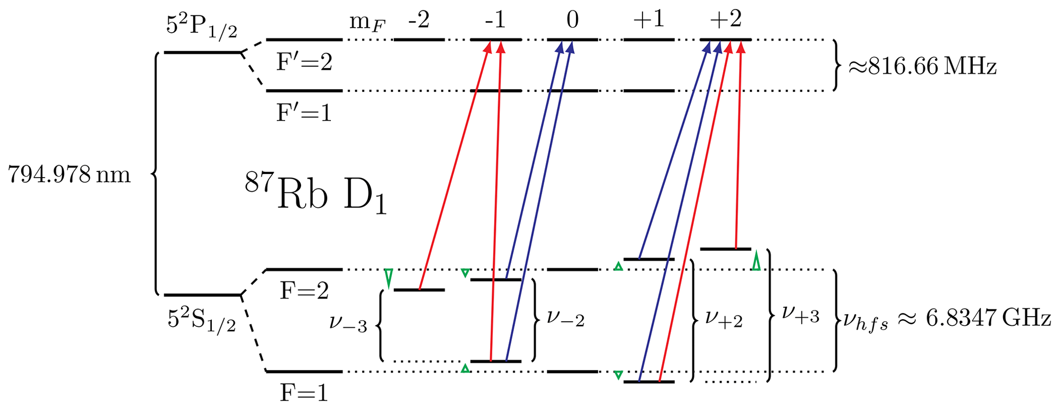
Figure 1Hyperfine structure of the 87Rb D1 line. The ambient magnetic field strength shifts the atomic energy states according to their mF quantum number (Steck, 2003). Two coherent excitations starting from two ground states to a common upper state, forming a Λ-system, are required to establish a CPT resonance. MAGSCA measures the Zeeman shifts of the ground states (F=1 and F=2) by establishing the red and blue Λ-systems. Thus, the Zeeman shifts are only depicted for the ground states and are indicated by the green triangles.
The bias current of the instrument's laser diode is modulated to create a multi-frequency modulated laser light field (Bjorklund et al., 1983; Amtmann et al., 2023) which is used to couple several CPT resonances within the rubidium vapour. This coupling enables a differential measurement principle to increase the instrument's accuracy. The detection frequency, which is used for measuring the Zeeman shift, is derived from the excitation of the clock transition within the 87Rb D1 line (Pollinger et al., 2018). This results in a low error of the detection frequency, translating to a magnetic field strength error of <0.001 nT.
The strengths of the individual atomic excitations depend on the angle between the magnetic field vector and the laser propagation direction (Vanier and Audoin, 1989), the so-called sensor angle β. As a consequence, two different sets of CPT resonances have to be used to cover the entire angular range and to enable the instrument's omnidirectionality (Pollinger et al., 2012). The blue Λ-systems (Fig. 1) are superposed to form the n2-coupled CPT resonance to measure the magnetic field strength at the sensor angular ranges of 0 to 60°, 120 to 240°, and 270 to 360°. For the complementary angular ranges (60 to 120° and 240 to 270°), the red Λ-systems are superposed to form the n3-coupled CPT resonance. For the instrument operation, the default angles for switching between the two sets are multiples of 60°.
The magnetic field strength B is derived from the difference in the resonance frequencies of a set of coupled CPT resonances, (red set in Fig. 1) or (blue set in Fig. 1), by applying the Breit–Rabi formula (Steck, 2003). The magnetic field strengths shift the difference frequency Δν2 by approx. 14 Hz nT−1 and Δν3 by approx. 21 Hz nT−1 (Pollinger et al., 2018). Due to this differential measurement, all coefficients corresponding to the even powers (B2, B4, B6, …) vanish in a Taylor series expansion of the Breit–Rabi formula. Thus, the most contributing series coefficient – besides the linear one – now corresponds to the cubic term B3. For MAGSCA the numerical value is Hz nT−3 for the blue set (Fig. 1) and Hz nT−3 for the red set (Fig. 1). This means for B=2000 nT the difference frequency deviates from the linear characteristic by −1.770 µHz (blue set) and −2.301 µHz (red set). Both are well below the frequency resolution (1 mHz) of the instrument. The consequence is a highly linear relationship between the magnetic field strength B and the frequencies Δν2 and Δν3 for the magnetic field strength range of the JUICE mission.
Not only the magnetic field, but also other effects, e.g. light shifts (Levi et al., 2000), can alter the atomic energy states. Under certain conditions, these are indistinguishable from Zeeman shifts (Amtmann, 2022). These effects are considered by the so-called heading characteristics, which are sensor-angle-dependent absolute errors and define the accuracy of the instrument. Figure 2 depicts an example of heading characteristics for the n2- and n3-coupled CPT resonances.
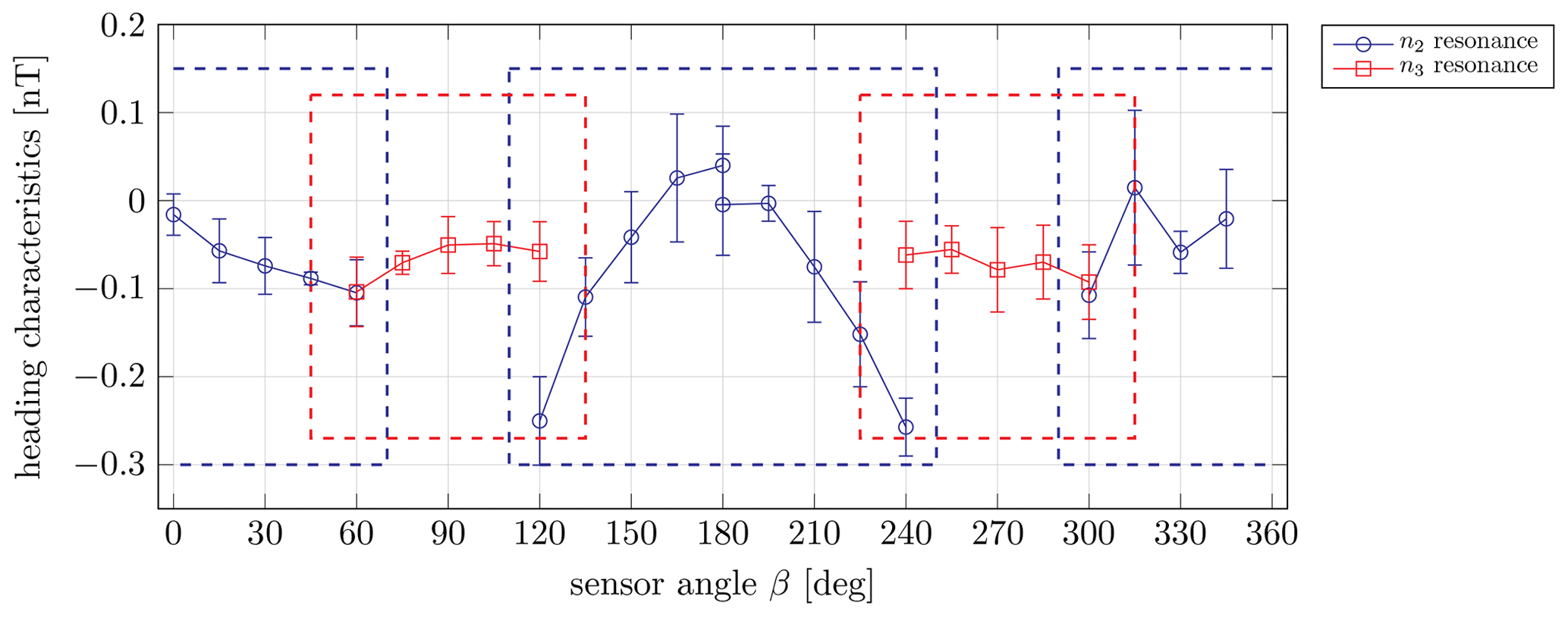
Figure 2Exemplary heading characteristics for the n2- and n3-coupled CPT resonances, which are sensor-angle-dependent absolute errors as a function of the sensor angle β. The angle β is the angle between the optical axis of the sensor unit and the magnetic field vector. MAGSCA can measure the magnetic field strength in the entire 360° angular range by switching between both resonances. For the angular ranges, where both coloured boxes overlap, an operation with both resonances is possible. The measurement setup is MAGSCA stand-alone (Sect. 2), with a laser bias current of 2.14 mA and a vapour cell temperature of 25 °C. Each depicted data point is the mean value of four separate measurements of the heading characteristics at four different sensor orientations, and the error bars are the corresponding standard deviations (see Sect. 4).
In 2018, the Coupled Dark State Magnetometer was launched into space for the first time on board the China Seismo-Electromagnetic Satellite (CSES) (Pollinger et al., 2018, 2020). The accuracy of this magnetometer was experimentally investigated in a Helmholtz coil system (operated at a constant applied magnetic field with a control loop based on a caesium magnetometer) at the Fragment Mountain Weak Magnetic Laboratory of the National Institute of Metrology in China (Pollinger et al., 2018). The peak–peak heading characteristics of approximately −2 to 1 nT were found. Post-processing was applied to the measured data to correct for the heading characteristics during the mission (Pollinger et al., 2020). For ground testing, the instrument can be operated at the sampling rate of 30 Hz, while the sampling rate is reduced to 1 Hz in orbit. The measured noise floor is lower than 50 pTrms Hz (Pollinger et al., 2018).
Figure 3 shows the MAGSCA flight model for the JUICE mission. The instrument's main components are the electronics box, the optical fibres, and the sensor unit. The laser unit, within the electronics box, is connected by an optical fibre to the sensor unit. The sensor unit houses a glass cell, containing the rubidium vapour. Here, the laser light probes the interaction of the magnetic field with the rubidium atoms. A second optical fibre guides the laser light back to the photo diode, mounted within the electronics box. A field-programmable gate array (FPGA) is responsible for signal generation and signal analysis (Pollinger et al., 2010).
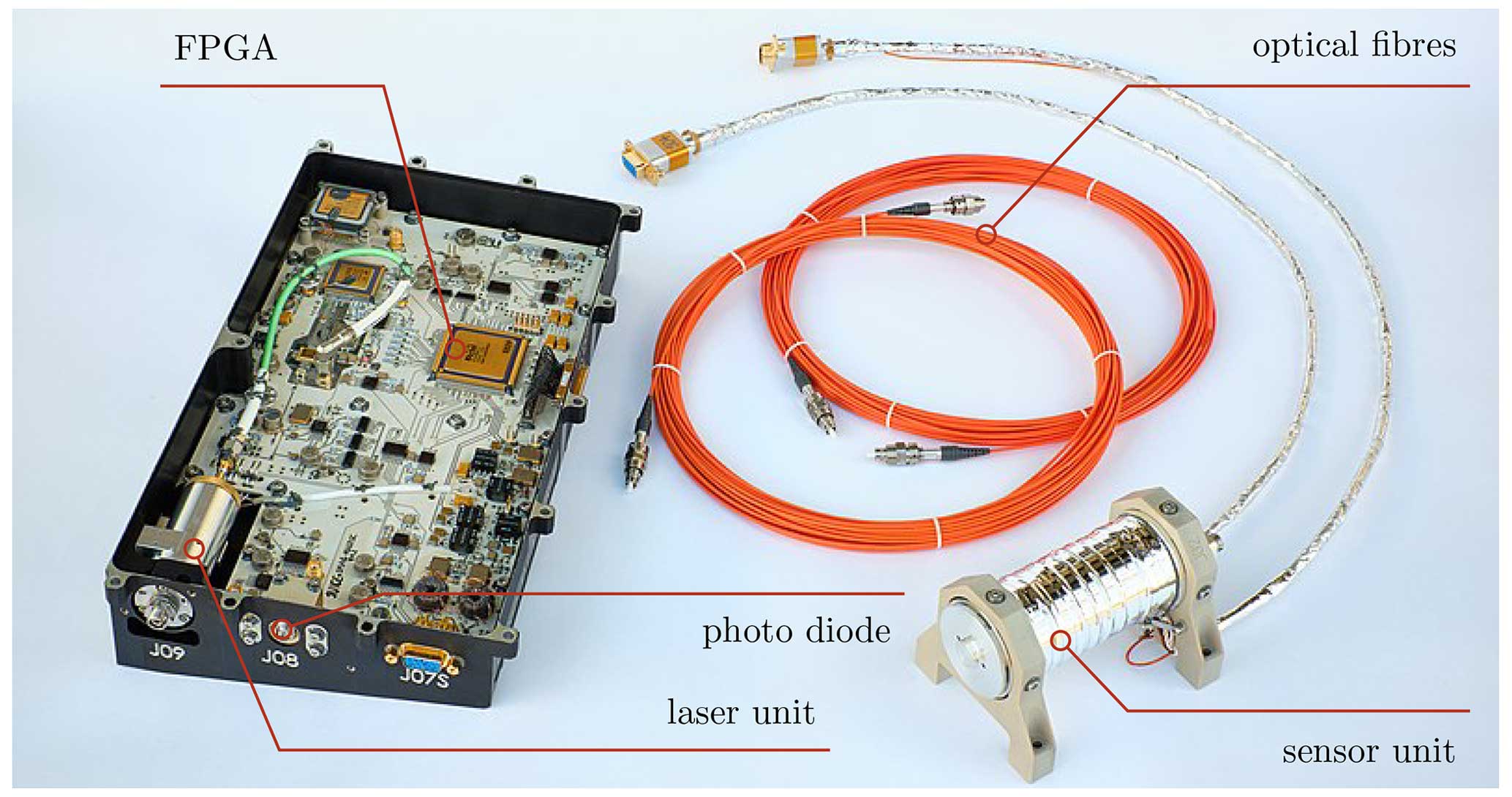
Figure 3The flight model for MAGSCA. The main components are labelled. © MAGSCA Team, Andreas Pollinger/https://w.wiki/3CHQ (last access: 12 June 2024)/CC BY 4.0.
For the JUICE mission, a new sensor unit which features a dual laser beam pass of the vapour cell was developed. A schematic drawing of the sensor unit is found in Ellmeier et al. (2023). The sensor unit itself does not contain magnetic materials. It mainly consists of aluminium, fibreglass-loaded PEEK, titanium, and glass. Each sensor component was carefully selected for its non-magnetic properties and was magnetically screened prior to assembly with the help of a three-axis high-resolution and low-noise fluxgate magnetometer (noise level < 10 pT Hz at 1 Hz, an engineering model of the DFG magnetometer of the NASA Magnetospheric Multiscale space science mission; Russell et al., 2014), including perming tests, in order to avoid any possible magnetisation of the unit. Compared to the previous sensor unit developed for the CSES mission, the new sensor unit increases the accuracy of the instrument by a reduction in the heading characteristics (Ellmeier et al., 2023; Ellmeier, 2019; Amtmann, 2022).
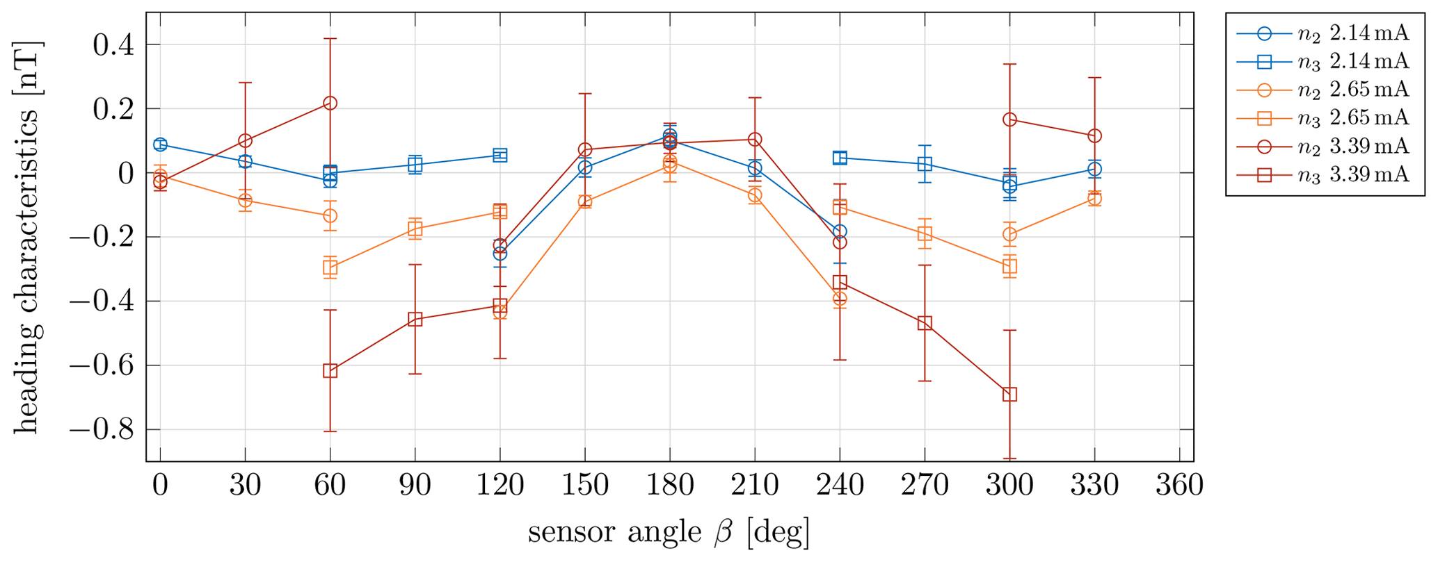
Figure 4Impact of various laser bias currents on the heading characteristics. The magnitude and the angular behaviour are changed. Measurements are taken with the MAGSCA stand-alone setup (see Sect. 2) at a vapour temperature of 25 °C. Each data point is the mean value of four separate measurements at four different sensor orientations, and the error bars are the corresponding standard deviations (see Sect. 4). The presented data have larger error bars at the laser bias current of 3.39 mA, which is mainly driven by the notable deviation of the residual field at the sensor position of 0° (Table 6).
All MAGSCA measurements presented within this work were recorded with a sampling rate of 128 Hz. Each data point of a heading characteristic is the mean value of the magnetic field strength recorded for 45 s at a constant sensor angle β and a constant magnetic field strength.
Section 4 discusses the measurement configuration for the heading characteristics of Figs. 2, 4, and 7. Each plotted data point is the mean value of four separate measurements of the heading characteristics at four different sensor orientations, with the same operational parameters. The error bars are the corresponding standard deviations.
1.2 Accuracy and precision
The accuracy and the precision of the magnetic field strength measurements are important for any kind of reference magnetometer. The accuracy of the instrument corresponds to the absolute error,
which is the deviation of the mean measured magnetic field strength B(β), averaged over a certain measurement time, from the true magnetic field strength B0 at the constant angle β. The precision P(β) is the noise of the magnetic field strength measurement at the constant angle β.
Due to the instrument's heading characteristics, the absolute error is a function of the sensor angle β. The precision depends on the slope of the amplitude of the selected coupled CPT resonance; thus, it can be dependent on the sensor angle β and the selected operational parameters like laser bias current and vapour temperature. The typical MAGSCA noise is between 15 and 25 pT Hz at 1 Hz.
The exemplary heading characteristics (Fig. 2) show that the deviations of the measurements depend on the selected coupled CPT resonance (n2 or n3). Additionally, the sensor angular behaviour of the heading characteristic and the magnitude of the heading characteristic are dependent on the operational parameters of MAGSCA. Parameters like laser bias current (and therewith linked modulation index and laser light intensity; Amtmann et al., 2023) and the rubidium vapour temperature influence the heading characteristics (Amtmann, 2022). The impact of different laser bias currents is shown in Fig. 4. For a proper correction of the magnetic field strength measurement, the heading characteristics have to be known for each set of operational parameters.
During the long time in space, the instrument's optical components (especially the optical fibres; Jernej et al., 2021) will experience radiation-induced attenuation. Based on radiation analysis and testing, in the worst case, the transmitted optical power at the end of the mission lifetime will be reduced to about one-quarter of the initially transmitted optical power. To counteract this, the instrument will be operated at higher laser bias currents and at higher vapour temperatures. Thus, the performance of the instrument has to be understood for these operational parameters.
During the main Ganymede science phase, JUICE will orbit the Jovian moon along two circular orbits with altitudes of 500 and 200 km. The measurements along several orbits will be taken for the in-flight calibration of the fluxgate sensors, which is based on MAGSCA data. During such a calibration sequence, it can be considered that MAGSCA measures the field strengths with an almost uniformly distributed sensor angle.
The accuracy of MAGSCA is determined by the heading characteristics which had to be characterised on ground. To quantify and compare different heading characteristics (measured at different operational parameters), the sensor angular-averaged accuracy and angular-averaged precision are introduced. They can be interpreted as averaging along an in-flight calibration sequence which includes measurements at all sensor angles.
The angular-averaged accuracy is defined as
It describes the deviation of the angular-averaged magnetic field strength measurement from the true magnetic field strength B0. The angular average of the magnetic field strength measurement is
determined for n measurements of B at n different, equally spaced sensor angles. Each Bi(β) is the mean of the magnetic field strength measurement of a 45 s time series at a constant sensor angle. The angular-averaged precision is calculated by computing the standard deviation for n values of Bi(β).
The heading characteristics have intrinsic angular behaviours, as shown in Fig. 2. Their magnetic field strength measurements, performed at evenly distributed sensor angles, do not reflect a normal distribution. Therefore, and do not represent the underlying statistical nature. However, they can be used as indicators for comparison between individual heading characteristics, measured with different operational parameters, and they can be considered to represent the achievable accuracy of the J-MAG instrument during the Ganymede phase of the mission.
To assess the measured heading characteristics with respect to the required accuracy for MAGSCA (σreq=0.2 nT), an accuracy rating is introduced in Table 1. The rating considers the angular-averaged accuracy and the angular-averaged precision , as well as the sum of the two parameters . This rating is used to determine the level of data post-processing for the investigated operational parameters. For the rating of A, the angular-averaged accuracy and the angular-averaged precision , as well as their sum , have to be within the required σreq range. The sum ensures that more than 68 % of the measured values are within the ±σreq interval (if a normal distribution of the heading characteristic values is assumed). For the rating of B, the angular-averaged accuracy and the angular-averaged precision are smaller than σreq, while their sum exceeds the limit. For the rating of C, the angular-averaged accuracy is below the σreq threshold, while and are larger than σreq. For the rating of D, all three are larger than the required range.
Table 1Requirements for the classification rating of the accuracy and precision of MAGSCA. The rating indicates the necessary level of post-processing for the MAGSCA data. The rating considers the angular-averaged accuracy and the angular-averaged precision , as well as the sum of the two parameters .
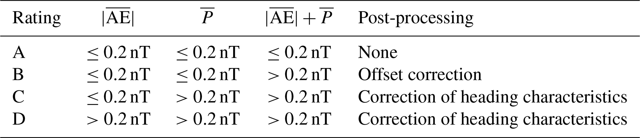
The four ratings define the required post-processing of the measured data. For a set of operational parameters with rating A, no data correction is necessary. All requirements are below the 0.2 nT threshold. Rating B requires an -based offset correction of the data in order to bring the measurements within the σreq range. As soon as the angular-averaged precision is larger than σreq, the heading characteristics have to be considered. For the ratings C and D, the complete data set has to be corrected by a function derived from the measured heading characteristics.
The verification tests aim to determine the accuracy of MAGSCA for several sets of operation parameters in the relevant magnetic field strength range (300 to 1500 nT) of the JUICE mission. The performance of each set of operational parameters has been evaluated concerning their required post-processing (see Table 1). The best-suited set of operational parameters will be defined as the default configuration for MAGSCA on JUICE.
The verification of the accuracy and precision of MAGSCA was performed at the geomagnetic Conrad Observatory (COBS) of GeoSphere Austria in Lower Austria. This geomagnetic observatory is part of the INTERMAGNET network (https://intermagnet.org/, last access: 15 March 2024) closely associated with the International Association of Geomagnetism and Aeronomy (IAGA). It features a magnetically clean and disturbance-free measurement environment (Leonhardt et al., 2020). For the verification tests, a Merritt coil system (Ferronato BM4-3000-3-A) was utilised, characterising the accuracy of the MAGSCA sensor unit over the entire sensor angular range and in the magnetic field strength range (300 to 1500 nT) required for the JUICE mission.
The coil system is located in the facilities tunnel system which has a constant ambient temperature of about 6°C year-round. This minimises thermal fluctuation experienced by the coils, which in turn reduces variations in the generated magnetic field.
Figure 5 shows a picture of the double Merritt coil system, located at the magnetically clean environment of the COBS tunnels. It consists of two independent coil systems. The first one is used to compensate the Earth's magnetic field (compensation coils). The Earth’s magnetic field at COBS is about 21 000 nT in the horizontal plane, and the vertical component is about 44 000 nT. The second system applies the magnetic field vector Bapp, which is required for testing MAGSCA. The applied field Bapp can be rotated electronically by software-controlled current sources for measuring the heading characteristics as a function of the sensor angle β.
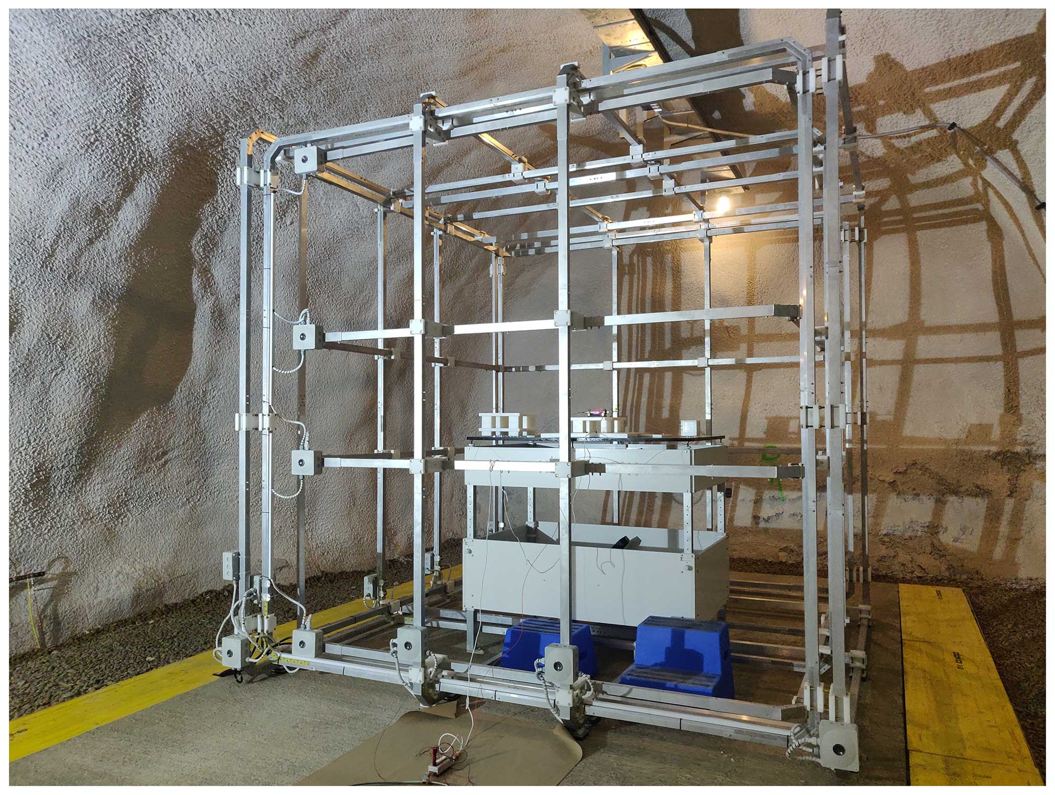
Figure 5Picture of the Merritt coil system within the tunnel of the Conrad Observatory. The side length of the cubic coil system is about 3 m. Each axis has two coil pairs with equal dimensions. This increases the homogeneity of the magnetic field and simplifies the handling of test setups.
The entire compensation system includes the fluxgate-based variometer of the observatory (located in a distance of about 300 m to the coil system), a set of current amplifiers, and the compensation coils. The system is not able to compensate the Earth's magnetic field exactly to zero. A small and slightly inhomogeneous residual magnetic field Bres remains. The inhomogeneity is caused by a small and practically unavoidable deformation of the Merritt coils. Table 2 lists the inhomogeneities of the compensated magnetic field along the three coil axes. The individual field components of the residual field are in the order of several nT; this is known from measurements with a fluxgate sensor.
Table 2Inhomogeneities of the magnetic field produced by the compensation coils (Merritt) along the three coil axes. The data were measured with a fluxgate sensor (engineering model for the DFG magnetometer of the Magnetospheric Multiscale mission (Russell et al., 2014)) by placing it in a −5, 0 and +5 cm grid along all three coil axes.
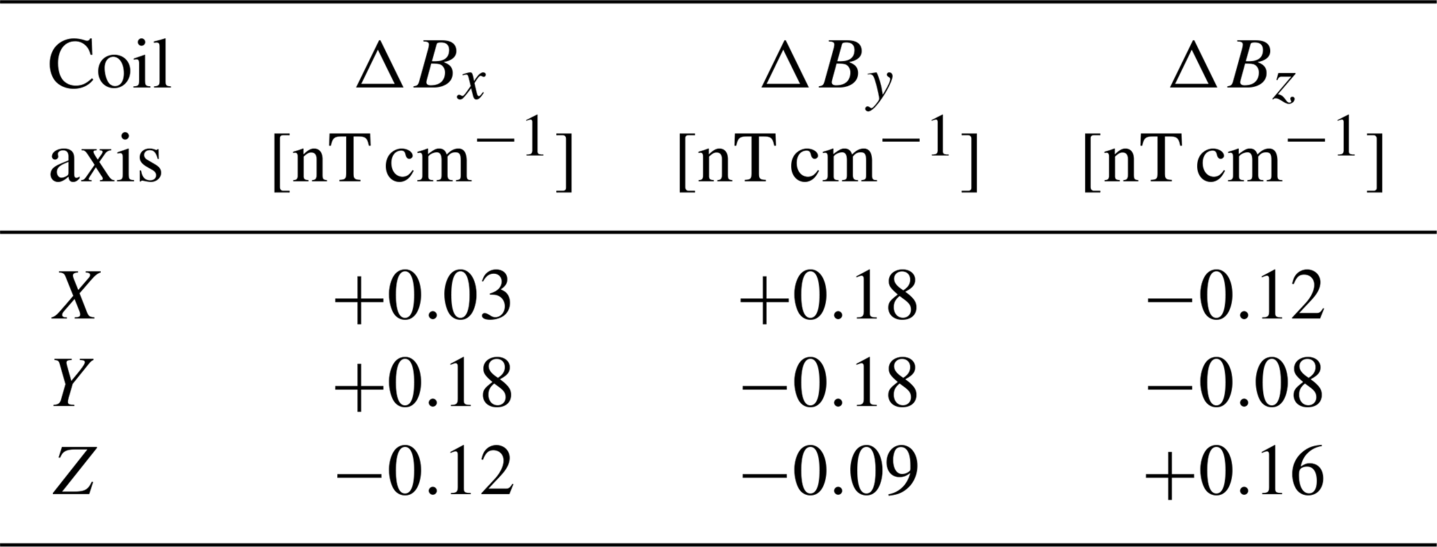
The maximum sensitive volume of the MAGSCA sensor unit is defined by the size of the cylindrical vapour cell, which has a diameter and length of 2.54 cm. Thus, the inhomogeneities in the order of 0.2 nT cm−1 have a significant influence on the magnetic field strength measurements. The magnetic field strength is averaged along the laser light path within the cell, effectively reducing the sensitive volume within the sensor unit. The two operational parameters, laser bias current (which defines the laser light intensity) and vapour temperature, impact the absorption of the laser light along the pass and, with this, the weighting function of the averaging. Therefore, the exact influence of the inhomogeneity on the magnetic field measurement is hard to assess. The inhomogeneities also require a precise placement of the sensor unit, within the centre of the coil system, to achieve reproducible measurements.
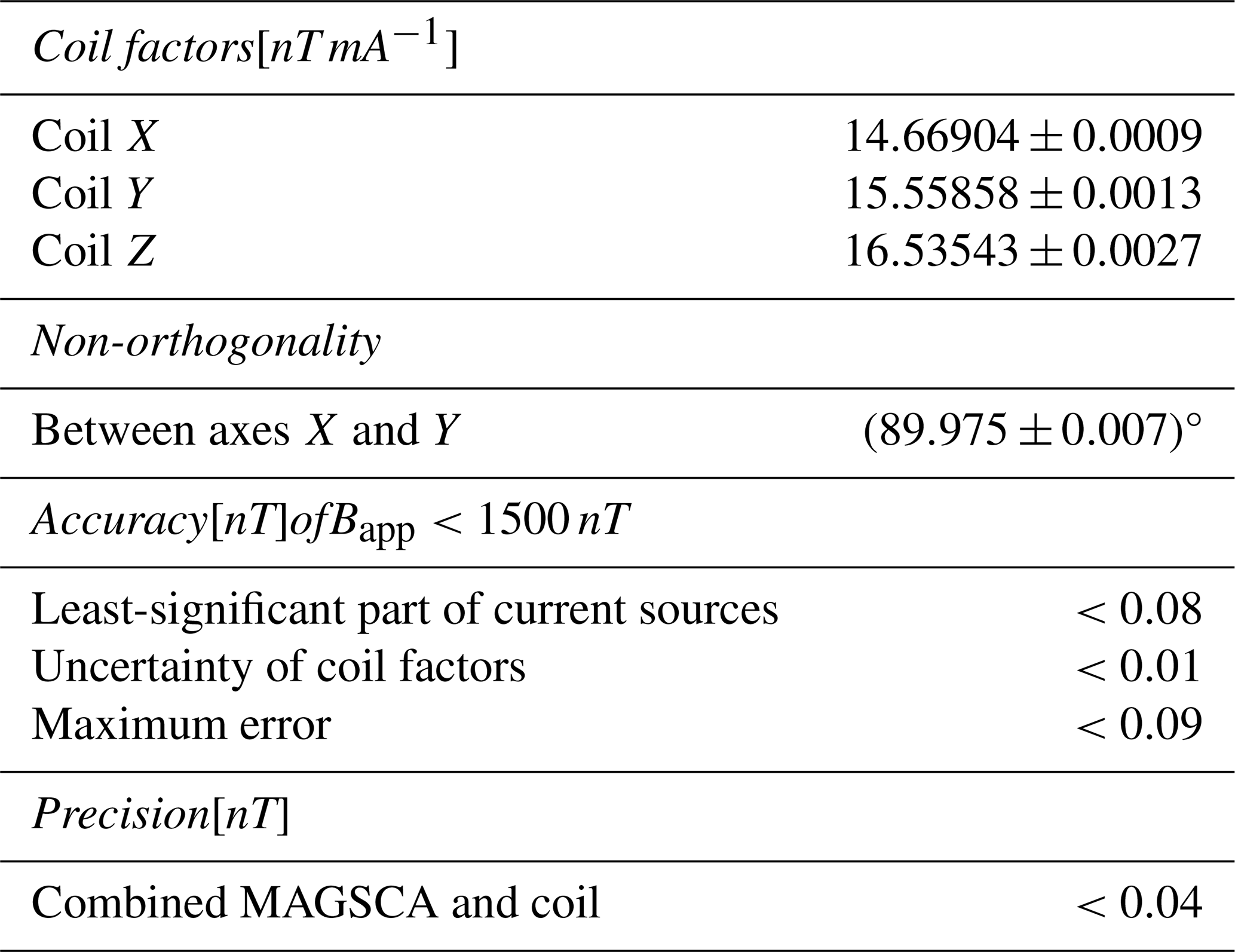
Table 3 lists the specifications of the Merritt coil system. The coil factors have been calibrated with an Overhauser magnetometer at large fields (>20 000 nT). The Overhauser magnetometer used (GSM-90 from GEM Systems) has an accuracy of 0.1 nT. For low applied field strengths (<1500 nT), the uncertainties of the coil factors result in an accuracy of the applied field below 0.01 nT. The current sources of the coil are BE2811 devices from iTest. The least-significant part of the current sources translates to a maximum error of 0.08 nT. Combined with the uncertainties of the coil factors for <1500 nT, the maximum error of the accuracy of the applied magnetic fields is <0.09 nT. The accuracy verification was carried out in the X–Y plane of the Merritt coil system (Fig. 5) to ensure the rotation and alignment of the sensor. Therefore, no additional test fields were applied in the Z direction. The non-orthogonality between the X and Y axes was experimentally determined to be (89.975±0.007)°.
Table 3Specifications of the double Merritt coil system at the Conrad Observatory.
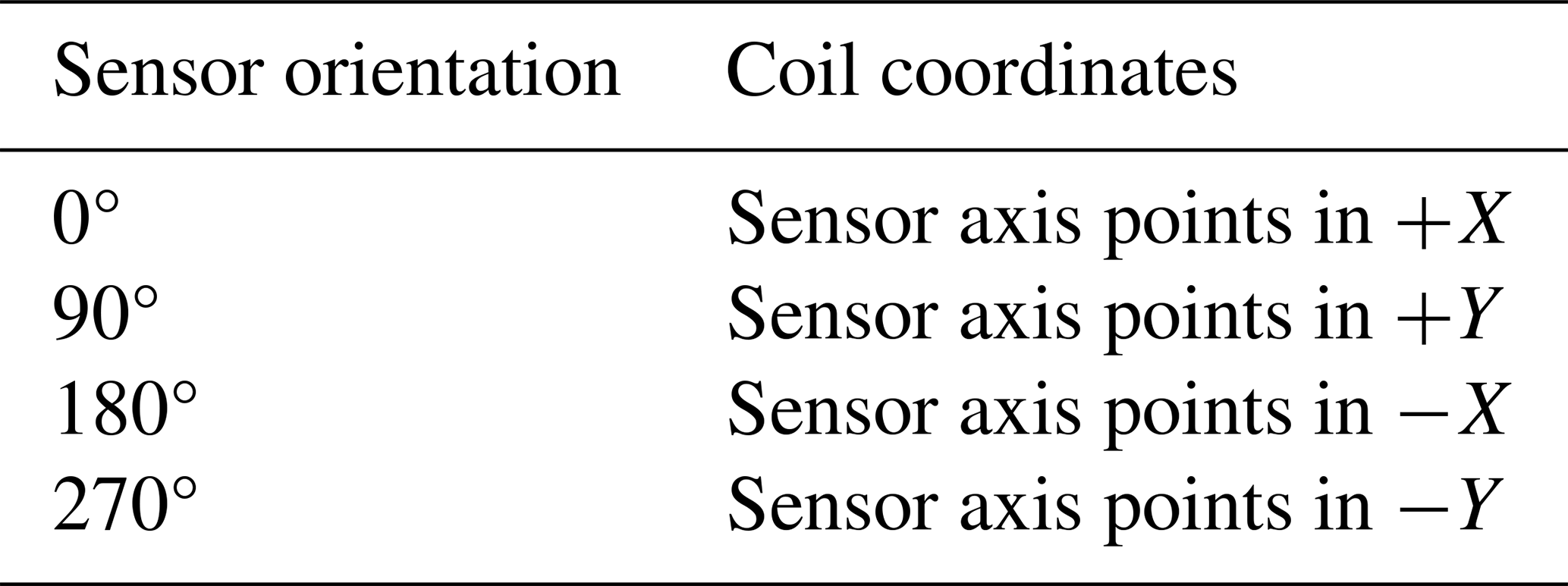
The heading characteristics were determined by a test routine consisting of four different sensor orientations. The four sensor orientations are required to separate the heading characteristics from the residual field Bres, as explained in Sect. 3. A sensor orientation is defined by the pointing direction of the sensor axis in relation to the coordinates of the coils. The sensor axis points along the sensor unit's cylinder axis away from the fibre connectors. In Fig. 6, the sensor axis is orientated in the −Y direction. Table 4 lists the definitions of all four sensor orientations. For the accuracy evaluation, measurements in all four sensor orientations were recorded right after each other to minimise drifts of the magnetic field within the coil system.
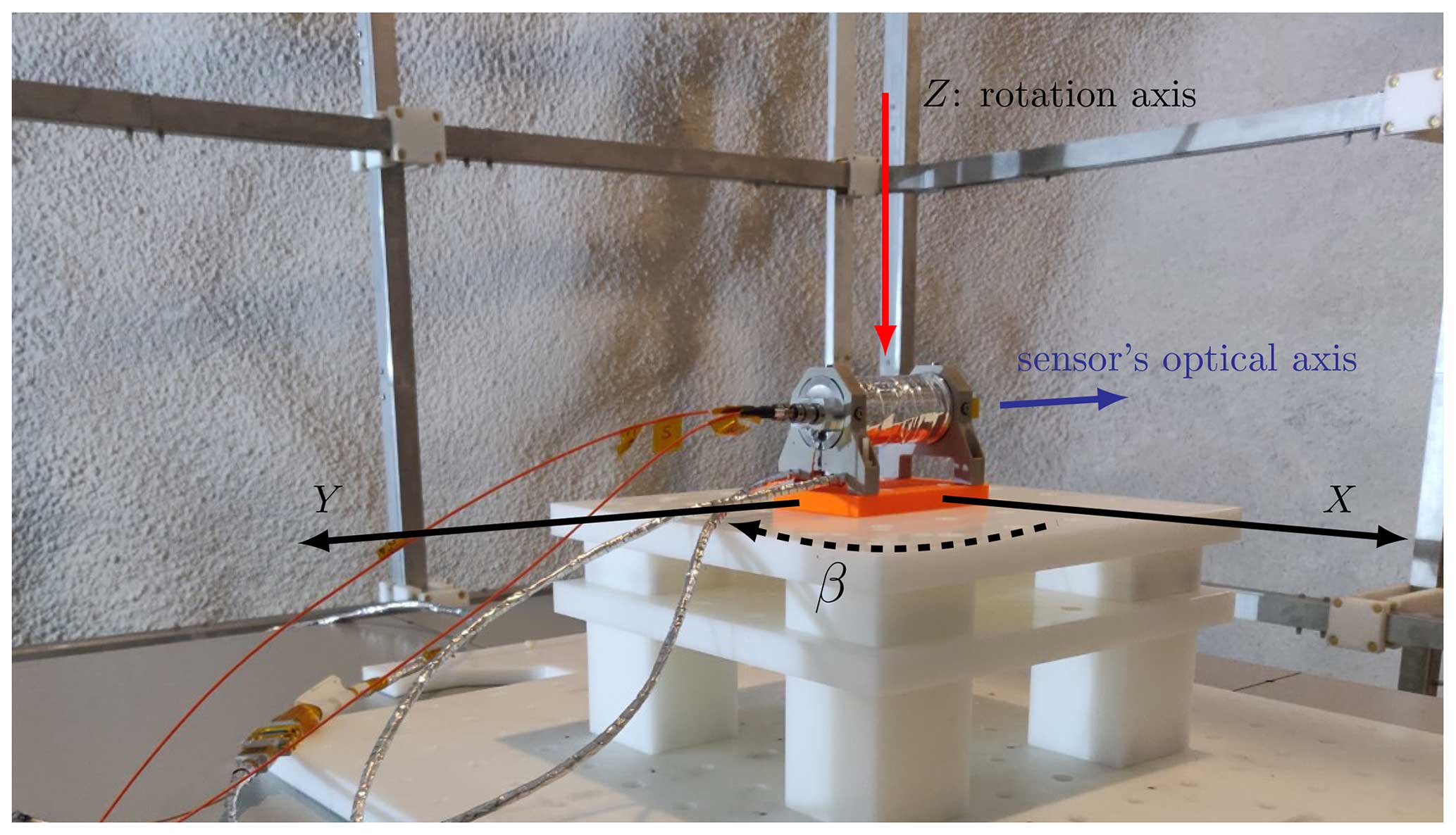
Figure 6The MAGSCA sensor is placed within the Merritt coil system. The coil axes are marked. The red axis is the rotation axis of the applied magnetic field vector and the rotation axis for the four different sensor orientations used within the coil system. In the configuration shown, the sensor's optical axis points along the axis direction of the −Y coil (blue arrow).
Table 4The definitions of the four sensor orientations within the Merritt coil system.
To evaluate the stability of the combined configuration of MAGSCA and the coil system, a magnetic field of 300 nT was applied in the X axis and was recorded for 10 h by MAGSCA (operational parameters: vapour temperature 25 °C and laser bias current 2.14 mA). The standard deviation of the time series was below 0.04 nT. The recording for each heading characteristic took between 15 and 25 min per sensor orientation; thus, the drift of the magnetic field strength can be neglected during one recording. Therefore, the noise and consequently the precision during the measurement of one heading characteristic is below 0.04 nT.
For each sensor orientation, the vapour cell and thus the illuminated volume covers a slightly different volume within the coil system. Therefore, a slightly different residual magnetic field strength is measured for each sensor orientation. This is caused by the field inhomogeneity in the order of 0.2 nT cm−1 (Table 2).
In the case where the rotation of the vapour cell is mechanically perfect and the cell always covers the same volume within the coil system, the magnetic field inhomogeneity of the residual field can be estimated: the sensitive volume (illuminated volume) within the vapour cell is about 2.5 cm along the sensor axis and about 2.0 cm perpendicular to the sensor axis. For a sufficiently large applied magnetic field, only the inhomogeneity in the applied magnetic field direction influences the measurement. For the sensor orientations 0 and 180°, the inhomogeneity is 0.08 nT in the axial +X direction and 0.36 nT in the perpendicular +Y direction. For the sensor orientations 90 and 270°, the inhomogeneity is −0.46 nT in the axial +Y direction and 0.36 nT in the +X direction. These values can be used as an estimate of the impact of the different sensor orientations on the magnetic field measurement.
Within the sensor housing, the vapour cell is offset from the rotation axis (Fig. 6) by about 0.5 cm along the sensor axis. Thus, the influence of the different sensor orientations is increased. For the sensor orientations 0 and 180°, the impact of the inhomogeneity is 0.10 nT in the axial +X direction and 0.36 nT in the perpendicular +Y direction. For the sensor orientations 90 and 270°, the impact of the inhomogeneity is −0.55 nT in the axial +Y direction and 0.36 nT in the perpendicular +X direction.
The MAGSCA flight model for the JUICE mission was tested with two different setups with the Merritt coil system: the MAGSCA stand-alone setup and the J-MAG-integrated setup.
In the MAGSCA stand-alone setup, MAGSCA is controlled by the MAGSCA-specific test hardware and software. This enables a fully automated execution of test sequences, which is supported by the Merritt coil system’s remote-control capabilities, since MAGSCA and the coil system can be simultaneously controlled by a custom-made software. With this combined setup, fast and automated measurements of heading characteristics are possible. This setup was used for measurements at laser bias currents of 2.14, 2.65, and 3.39 mA; sensor temperatures of 25, 35, and 45 °C; and at an applied magnetic field strength of 300 nT. For the MAGSCA stand-alone setup, the heading characteristics were sampled with the equidistant sensor angle steps of 15°.
For the J-MAG-integrated setup, the MAGSCA front-end electronics are installed within the J-MAG electronics box. The data communication is no longer handled with the MAGSCA-specific test setup. In this configuration, the magnetic field vector rotation requires a manual interaction with the interface software of the Merritt coil system, which increases the testing time per heading characterisation. However, this is the flight configuration on board the JUICE spacecraft. The J-MAG-integrated setup was used for measurements at a laser bias current of 2.14 mA and a sensor temperature of 25 °C at applied magnetic field strengths of 300, 900, and 1500 nT. For the J-MAG-integrated setup an adapter plate was used to correct the vapour cell offset of 0.5 cm within the sensor unit along the optical path. The heading characteristics for this setup were sampled with the equidistant sensor angle steps of 30°.
The MAGSCA front-end electronics and the J-MAG electronics box were placed at a distance of more than 7 m from the Merritt coil system to prevent interference with the MAGSCA sensor unit located in the centre of the Merritt coil system.
For all measurements, the modulation frequency of the control loop for the microwave reference stabilisation was set to 919 Hz, and the modulation frequency of the control loop for the magnetic field strength measurement was set to 337 Hz.
The data processing approach aims to separate the heading characteristics from the effective magnetic field by fitting a mathematical model to the measured data (Amtmann, 2022). Simultaneously, it allows determining the potential remanent magnetisation of the sensor unit. From the heading characteristics, the angular-averaged accuracy and angular-averaged precision can be calculated to evaluate the performance of MAGSCA.
The approach follows these steps:
-
modelling of the effective magnetic field;
-
creation of a fit function and the reduction of fit parameters;
-
measurements at four different sensor orientations and fitting of data;
-
evaluation of remanent magnetisation of the sensor unit;
-
calculation of angular-averaged accuracy and angular-averaged precision.
3.1 Model of effective magnetic field
The instrument measures the sum of its heading characteristics Bhead and the effective magnetic field strength:
The effective magnetic field Beff is determined by the sum of the applied field Bapp and the residual field Bres:
Thus, the heading characteristics are calculated by
For calculating the heading characteristics, the applied and the residual field have to be known.
For the accuracy verification, the applied magnetic field is rotated around the Z axis by the Merritt coil system (Fig. 6). This rotational behaviour (rotating vector) can be expressed by
The parameters aX and aY are the maxima of the applied field strengths in the X and Y directions, which are characterised by their respective coil factors, and β represents the field direction in the X–Y plane. The angle β corresponds to the sensor angle introduced in Sect. 1.1. bX and bY describe the influences of the non-orthogonality between the X and Y axes of the coil system on the applied field Bapp. The parameter bY describes the impact in the X direction of a magnetic field applied with the Y-axis coil, and bX is the impact in the Y direction of a magnetic field applied with the X-axis coil. The non-orthogonality of the coil's Z axis is not considered, since no field was applied along this axis.
By adding the residual field to the applied field, the effective field becomes
The scalar magnetometer measures the magnetic field strength; therefore, the absolute amplitude is of interest. The squared norm is
3.2 Fit function and reduction of fit parameters
Measurements with a fluxgate (engineering model of the DFG magnetometer developed for the Magnetospheric Multiscale mission; Russell et al., 2014) showed that the individual field components of the residual field are of the order of several nT. However, their exact values are not known; thus, the effective magnetic field cannot simply be removed from the measured magnetic field strength Bmeas (see Sect. 2). The effective field can be determined by fitting the measured magnetic field strength Bmeas with Eq. (9). This equation is simplified by using 2cos βsin β=sin (2β) and .
With the coefficients
the fit function becomes
Equation (15) shows that the fit coefficients ki are linearly independent due to their trigonometric functions of β. From the ki coefficients, the unknowns of Eqs. (10)–(14) have to be determined. To allow this and to avoid overfitting of the model, the number of unknown parameters impacting fcoil(β,k) is reduced by the following assumptions.
The residual field component Bz appears only independently in k1. For the fit routine, this factor will be interpreted as a variable offset and will be treated accordingly: some offset of the heading characteristics is “put” into Bz by the fit routine. This must be avoided for the correct evaluation of the angular-averaged accuracy . To prevent this, the parameter Bz is removed. This is a valid approximation because Bz is small compared to and will not change k1 significantly.
For example, an applied magnetic field of and a residual field of result in the magnitude of 300.002 nT for orthogonal coils . For an applied field in the X–Y direction, a small residual field in Z has nearly no impact on the magnetic field strength measured by the scalar magnetometer.
The fit parameters bX and bY are determined by the non-orthogonality between the X and Y coils; therefore, they are regarded as the same (). For applied magnetic fields <2000 nT the approximation can be made. The accuracies of the coil are high (see Table 3); thus, a=afix is set to the fixed value for the applied magnetic field strength.
To summarise, the reduced coefficients become
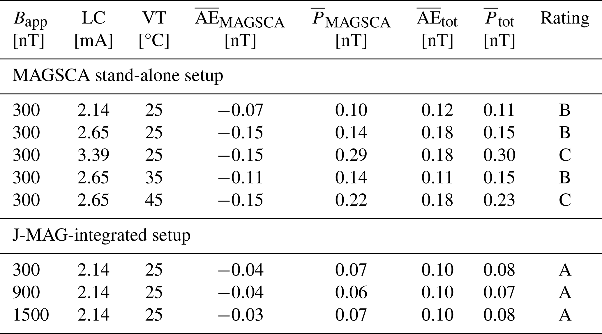
Table 5Angular-averaged accuracy and angular-averaged precision of MAGSCA on board JUICE. The total angular-averaged accuracy and the total angular-averaged precision consider the accuracy and precision of the Merritt coil system used for applying the reference magnetic field. The operational parameters are the laser bias current (LC) and the vapour temperature (VT) at the applied magnetic field strength Bapp. and are rated according to the classification introduced in Table 1.
3.3 Measurement at four different sensor orientations and fitting of data
A robust separation of Beff (coil-driven) and Bhead (MAGSCA-driven) is of interest. This is achieved by a successive 90° rotation of the sensor unit within the coil system with recordings of Bmeas where the applied magnetic field is rotated around Z for each sensor orientation. The 90° rotation is achieved with the help of four alignment pins assembled to the sensor base plate, forming a 5 cm-by-5 cm square. These alignment pins fit tightly into four holes of the measurement table whose position is fixed within the coil system. For changing the sensor orientation, the sensor with the pins attached is lifted out of the alignment holes, rotated by 90°, and re-inserted into the same four holes. With the fit accuracy of the alignment pins within the holes, an angular positioning error of less than 0.5° is achieved. This is small enough in order not to contribute to any significant errors in the fitting. The coil's effective field Beff does not change while the heading characteristic Bhead is phase-shifted by 90° relative to Beff for each sensor orientation. These individual phase shifts for β are added to the fit functions. The sensor orientations used for this approach are listed in Table 4.
As discussed in Sect. 2, each sensor orientation has a slightly different residual field. This has to be taken into account during fitting. Four sets of residual field fit parameters (, with ) are applied to the fit function fcoil of Eq. (15).
For a given set of operational parameters, all heading characteristics (measured at the four sensor orientations) are fitted with the parameter b, while each sensor orientation has its own fit parameters for their respective residual field (, ).
3.4 Evaluation of remanent magnetisation of the sensor unit
The fit gives four residual fields. If the differences between these fields are larger than the expected inhomogeneity, a remanent magnetisation of the sensor unit is probable. In this case, the fit interprets the magnetisation as a residual magnetic field within the coil system, and the variations in the fitted residual field become larger than the inhomogeneities within the coil system.
A sensor unit with a remanent magnetisation can only be reasonably fitted with a single residual field for all four sensor orientations to extract the heading characteristics.
3.5 Calculation of accuracy and precision
From the measured data for both coupled CPT resonances and the fit results, the angular-averaged accuracy
is calculated. The angular-averaged precision is the corresponding standard deviation.
The total angular-averaged accuracy and total angular-averaged precision not only depend on MAGSCA but also on the accuracy and precision of the reference magnetic field strength Beff produced by the Merritt coil system (Table 3). The total angular-averaged accuracy, including the accuracy of the Merritt coil system , is
The total precision, including the precision of the Merritt coil system , is
In the course of the evaluation of the accuracy and precision of MAGSCA, several sets of operational parameters were investigated. One set of operational parameters consists of a laser bias current and a sensor temperature, measured at different applied magnetic field strengths. For each set of operational parameters and for each sensor orientation, the applied magnetic field was rotated and recorded.
The operational parameters and the fit results for calculating the effective field Beff are listed for the MAGSCA stand-alone setup in Table 6 and for the J-MAG-integrated setup in Table 7.
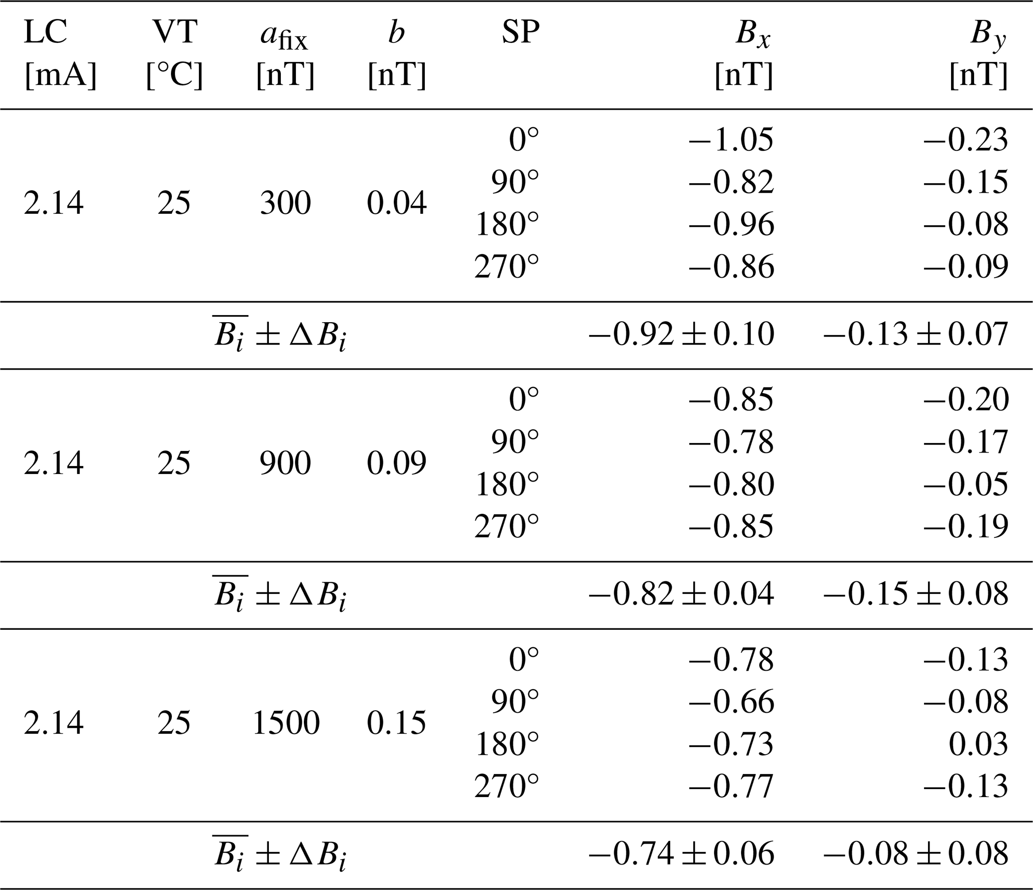
Table 6Fit parameter for the calculation of Beff for the MAGSCA stand-alone setup within the Merritt coil system. The fit results were used to determine the heading characteristics at various laser bias currents (LCs) and vapour temperatures (VTs). afix is the applied magnetic field strength, and b is the impact of the non-orthogonality. The residual fields are listed as Bx and By for each sensor orientation (SO). The mean values and their standard deviations ΔBi were calculated for each component of the residual magnetic fields. Due to errors in the data recording, the sensor orientation of 90° at 35 °C vapour temperature and the sensor orientation of 180° at 45 °C vapour temperature had to be removed from the data evaluation.
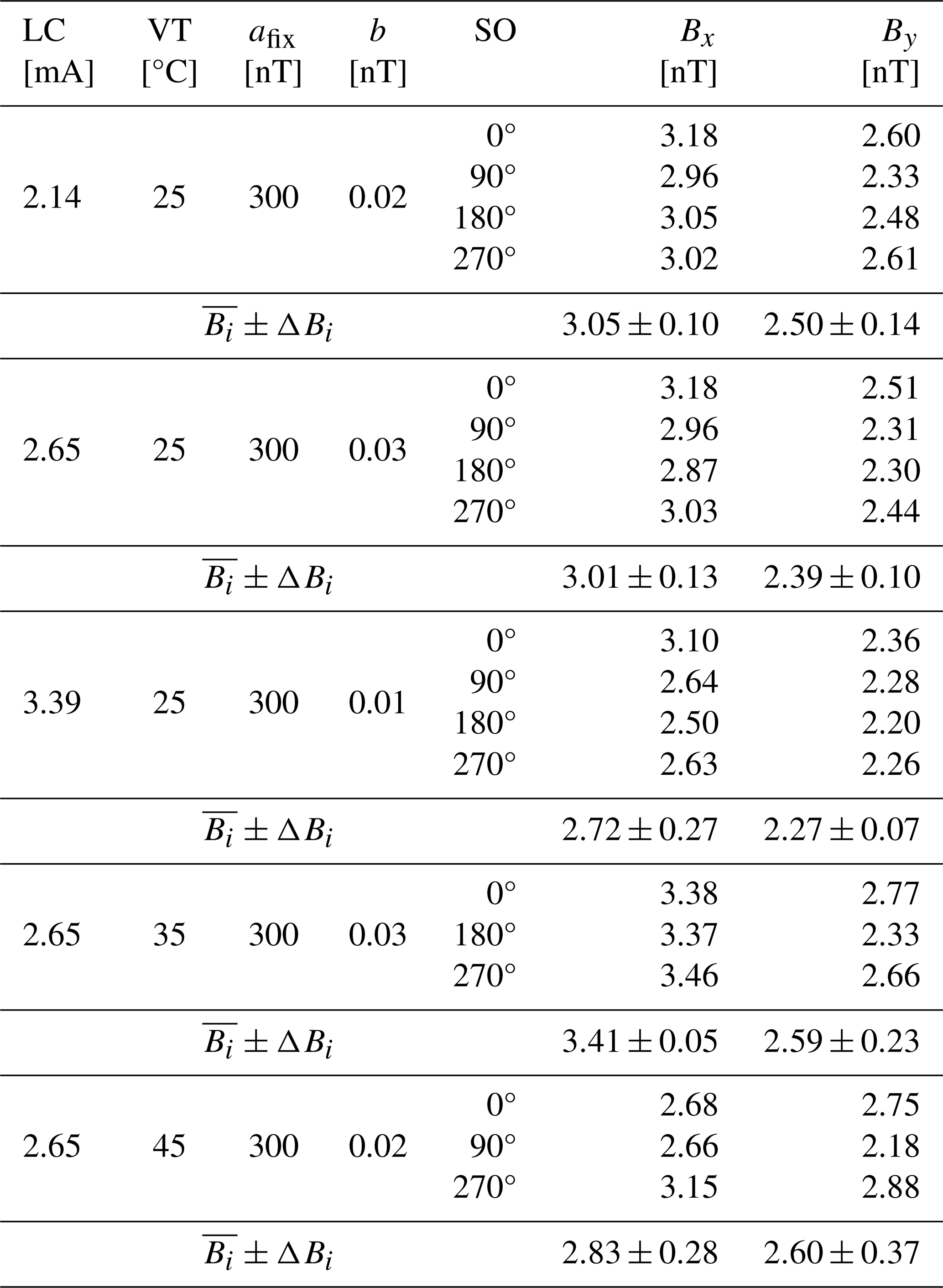
Table 7Fit parameter for the calculation of Beff for the J-MAG-integrated setup within the Merritt coil system. The fit results were used to determine the heading characteristics at various laser bias currents (LCs) and vapour temperatures (VTs). afix is the applied magnetic field strength, and b is the impact of the non-orthogonality. The residual fields are listed as Bx and By for each sensor orientation (SO). The mean values and their standard deviations ΔBi were calculated for each component of the residual magnetic fields. The variations in the residual fields are smaller compared to the MAGSCA stand-alone setup due to the compensation of the vapour cell offset by the adapter plate.
For the measurements at the sensor temperatures of 35 and 45 °C (Table 6), only three sensor orientations are listed. During the data recording of the missing sensor orientations, an error occurred; thus, the measurements had to be removed. This increases the uncertainty of the fitted residual fields and consequently of the calculated heading characteristics.
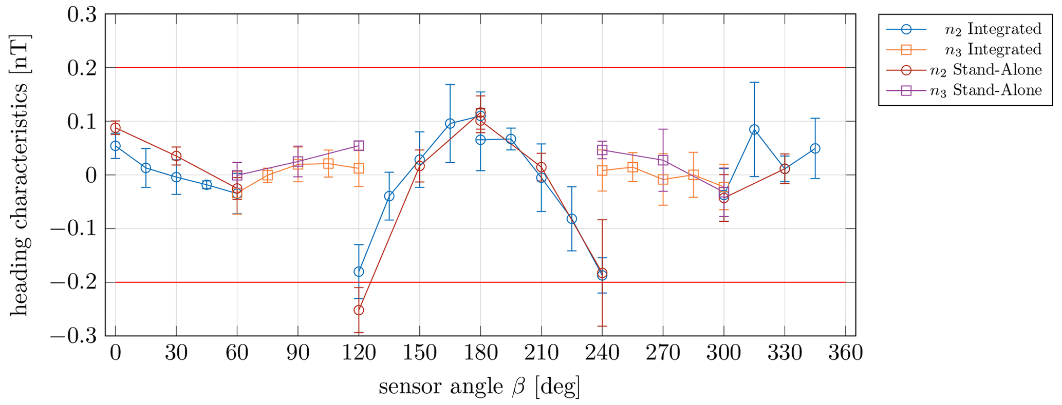
Figure 7Heading characteristics Bhead of the n2- and n3-coupled CPT resonances measured with the MAGSCA stand-alone setup and the J-MAG-integrated setup. Operational parameters: the bias current 2.14 mA, and the sensor cell temperature is 25 °C at Bapp=300 nT. Each data point is the mean value of four separate measurements at four different sensor orientations, and the error bars are the corresponding standard deviations. The fit parameters for calculating the effective field Beff can be found in Tables 6 and 7. The accuracy requirement 0.2 nT (1σ) of the JUICE mission is added as red horizontal lines.
A remanent magnetisation of the sensor unit does not depend on the selected set of operational parameters; thus, only fit results for all four sensor orientations are considered for the evaluation of a potential sensor magnetisation. At the laser bias current of 2.14 mA (Tables 6 and 7), the standard deviations ΔBi of both components of the residual fields are in the order of 0.10 nT. These variations are similar to or smaller than the expected impact of the inhomogeneities on the magnetic field strength measurement (Sect. 2). Thus, it can be concluded that the MAGSCA sensor unit does not have a residual magnetisation larger than 0.10 nT. Additionally, the adapter plate, used for the spatial correction of the vapour cell offset, reduces the variations in the residual fields in the J-MAG-integrated setup.
From the afix and b parameters of Tables 6 and 7 the mean non-orthogonality angle was calculated as (89.995±0.002)°. A small deviation was found compared to the measured non-orthogonality angle of (89.975±0.007)°. This can be explained by the uncertainty of the fitting approach used and/or by a possible change in the deformation of the Merritt coil system between the time of the experimental determination of the non-orthogonality and the time of the verification of MAGSCA.
The results of Tables 6 and 7 were used to subtract the applied magnetic field from the measured data to extract the heading characteristics. In order to have a clear visualisation of each set of operational parameters, combined heading characteristics were determined. Therefore, the mean value of the four heading characteristics and their standard deviation were calculated for each sensor angle. Thus, the presented Figs. 2, 4, and 7 show the combined heading characteristics for the respective sets of operational parameters. The standard deviation is used for the error bars.
The variations in the residual fields at the high laser bias current of 3.39 mA seen in Table 6 is mainly driven by the notable deviation of the residual field at the sensor orientation of 0°. This also explains the larger error bars of the combined heading characteristics in Fig. 4 for the laser bias current of 3.39 mA.
The combined heading characteristics were used to calculate the angular-averaged accuracy and the angular-averaged precision . The accuracy and precision of the Merritt coil system (Table 3) was considered by Eqs. (22) and (23) to determine the total angular-averaged accuracy and total angular-averaged precision. All results are found in Table 5 and are rated according to the classification of Table 1.
Figure 7 depicts the heading characteristics for the laser bias current of 2.14 mA, the sensor temperature of 25 °C, and the applied magnetic field strength of 300 nT. The figure shows that the stand-alone setup and the J-MAG-integrated setup result in heading characteristics with the same angular behaviour. This set of operational parameters satisfies the performance requirements and is rated with A for the J-MAG-integrated setup (Table 1). It is the most suitable set of investigated operational parameters for MAGSCA. No correction of the data is required to comply with the required performance for the JUICE missions. Table 5 shows that the stand-alone and integrated setups result in comparable angular-averaged accuracies and angular-averaged precisions. Thus, the performance of the stand-alone setup can be expected in flight for the other sets of operational parameters.
The applied magnetic field strength in the tested magnetic field range (300–1500 nT) does not impact the accuracy and precision of MAGSCA.
A higher laser bias current has a negative effect on the accuracy and precision which can be explained by larger light shift effects due to the higher light intensity within the vapour cell (Amtmann, 2022). The ratings for the measurements at the sensor temperatures 35 and 45 °C are impacted by the lack of a fourth sensor orientation; however, it is concluded that a higher vapour temperature results in a lower rating.
The angular-averaged accuracy of Table 5 is lower than the applied magnetic field strength. It is assumed that the imbalance of the individual components of the laser light spectrum (created by the modulation of the laser bias current), together with their frequency detuning to their respective atomic transitions, cause light shifts in the atomic levels involved in the formation of the CPT resonances. Under certain conditions, these light shifts are indistinguishable from Zeeman shifts (atomic-level shifts created by the ambient magnetic field) which cause the heading characteristics and the overall offset of the magnetic field strength measurement (Amtmann, 2022).
The accuracy of MAGSCA below the ambient magnetic field strength of 300 nT will be discussed in a separate publication.
This paper reports the pre-flight verification of the accuracy and precision of the magnetic field strength measurement of the scalar magnetometer (MAGSCA) on board ESA's Jupiter Icy Moons Explorer (JUICE) mission. The performance was evaluated with a double Merritt coil system at the Conrad Observatory in Lower Austria.
The deficiencies of the applied test field and MAGSCA's heading characteristics were separated by measurements with four dedicated sensor orientations and by fitting a mathematical model to the measured data. The heading characteristics describe variations in the magnetic field strength measurement from a reference magnetic field strength as a function of the angle between the sensor axis and the applied magnetic field vector. It was found that the accuracy and precision of MAGSCA are determined by the heading characteristics, which in turn depend on the selected set of operational parameters.
It was shown that the operation of the magnetometer at a laser bias current of 2.14 mA and a sensor temperature of 25 °C does not require data correction to be compliant with the accuracy requirement of 0.2 nT (1σ) for the JUICE mission. Therefore, these operational parameters were defined as the default configuration of MAGSCA.
Especially in the Jupiter environment, the instrument's optical components will experience radiation-induced attenuation. To counteract this, the instrument will have to be operated at higher laser bias currents and at higher sensor temperatures. Thus, the performance of the instrument has to be understood for these operational parameters.
For the investigated operational parameters, the applied magnetic field strength does not have an impact on the accuracy and precision of MAGSCA in the tested range from 300 to 1500 nT. Additionally, no measurable residual magnetisation of the sensor unit was found. A comparison of the stand-alone setup and the integrated setup shows that the same result as measured with the stand-alone setup can be expected for MAGSCA during the JUICE mission.
In a future publication, we will discuss the impact of radiation-induced attenuation within the optical path on the performance of the scalar magnetometer on JUICE and the in-flight tracking of this attenuation.
The data and the fitting software that support the findings of this study are available from the corresponding authors upon reasonable request.
CA prepared the article with contributions from PB, WM, MD, EE, and RL. The experiments were designed by CA, AB, RL, WM, AP, and JW and were carried out by CA, AB, RB, and AS. The MAGSCA flight hardware was build by AP, CH, MA, CA, AB, RL, and IJ.
The contact author has declared that none of the authors has any competing interests.
Publisher's note: Copernicus Publications remains neutral with regard to jurisdictional claims made in the text, published maps, institutional affiliations, or any other geographical representation in this paper. While Copernicus Publications makes every effort to include appropriate place names, the final responsibility lies with the authors.
The authors would like to thank Roman Leonhardt and his team for providing and maintaining the infrastructure at the Conrad Observatory, which was a crucial element for the required measurement campaigns.
The authors are grateful for financial support from the Austrian Space Applications Programme (grant nos. 840122 and 873688) of the Austrian Research Promotion Agency and the PRODEX Programme of the European Space Agency (grant no. 4000114669). The investigation of the heading characteristics and the linked understanding of the handling of the double Merritt coil systems play an important role in the investigation of a novel vector magnetometer concept. This novel approach is based on the Coupled Dark State Magnetometer and is currently in development, which is funded by the 1000 Ideas Programme of the Austrian Science Fund (FWF) with grant ref. TAI 823. For open-access purposes, the authors have applied a CC BY public copyright licence to any author-accepted manuscript version arising from this submission. This work was supported by the TU Graz Open-Access Publishing Fund.
This paper was edited by Lev Eppelbaum and reviewed by two anonymous referees.
Acuña, M. H.: Space-based magnetometers, Rev. Sci. Instrum., 73, 3717–3736, https://doi.org/10.1063/1.1510570, 2002. a
Amtmann, C.: Heading Characteristics of the Coupled Dark State Magnetometer and their Sources, PhD thesis, Graz University of Technology, Graz, https://repository.tugraz.at/publications/marc21/ngqwx-t5e38/preview/80471.pdf (last access: 12 June 2024), 2022. a, b, c, d, e, f
Amtmann, C., Lammegger, R., Betzler, A., Agú, M., Ellmeier, M., Hagen, C., Jernej, I., Magnes, W., Pollinger, A., and Ernst, W. E.: Experimental and theoretical investigations on the modulation capabilities of a sample of vertical cavity surface emitting laser diodes for atomic vapour applications, Appl. Phys. B, 129, 31, https://doi.org/10.1007/s00340-023-07971-7, 2023. a, b
Arce, A. and Rodriguez, D.: Juice Magnetometer Boom Subsystem, in: Proc. 18th European Space Mechanisms and Tribology Symposium 2019, 18–20 September 2019, Munich, Germany, https://esmats.eu/esmatspapers/pastpapers/pdfs/2019/arce.pdf (last access: 12 June 2024), 2019. a
Arimondo, E.: V Coherent Population Trapping in Laser Spectroscopy, Prog. Optics, 35, 257–354, https://doi.org/10.1016/S0079-6638(08)70531-6, 1996. a
Auster, H.-U.: How to measure earth’s magnetic field, Phys. Today, 61, 76–77, https://doi.org/10.1063/1.2883919, 2008. a
Balogh, A.: Planetary Magnetic Field Measurements: Missions and Instrumentation, Space Sci. Rev., 152, 23–97, https://doi.org/10.1007/s11214-010-9643-1, 2010. a
Bjorklund, G. C., Levenson, M. D., Lenth, W., and Ortiz, C.: Frequency modulation (FM) spectroscopy, Appl. Phys. B, 32, 145–152, https://doi.org/10.1007/BF00688820, 1983. a
Ellmeier, M.: Evaluation of the Optical Path and the Performance of the Coupled Dark State Magnetometer, PhD thesis, Graz University of Technology, Graz, Austria, https://diglib.tugraz.at/evaluation-of-the-optical-path-and-the-performance-of-the (last access: 12 June 2024), 2019. a
Ellmeier, M., Amtmann, C., Pollinger, A., Magnes, W., Hagen, C., Betzler, A., Jernej, I., Agú, M., Windholz, L., and Lammegger, R.: Frequency shift compensation for single and dual laser beam pass sensors of a coherent population trapping resonance based coupled dark state magnetometer, Measurement: Sensors, 25, 100606, https://doi.org/10.1016/j.measen.2022.100606, 2023. a, b
Grasset, O., Dougherty, M. K., Coustenis, A., Bunce, E. J., Erd, C., Titov, D., Blanc, M., Coates, A., Drossart, P., Fletcher, L. N., Hussmann, H., Jaumann, R., Krupp, N., Lebreton, J. P., Prieto-Ballesteros, O., Tortora, P., Tosi, F., and Van Hoolst, T.: JUpiter ICy moons Explorer (JUICE): An ESA mission to orbit Ganymede and to characterise the Jupiter system, Planet. Space Sci., 78, 1–21, https://doi.org/10.1016/j.pss.2012.12.002, 2013. a
Hussmann, H., Palumbo, P., Jaumann, R., Dougherty, M., Langevin, Y., Piccioni, G., Barabash, S., Wurz, P., van den Brandt, P., Gurvits, L., Bruzzone, L., Plaut, J., Wahlund, J., Cecconi, B., Hartogh, P., Gladstone, R., Iess, L., Stevenson, D., Kaspi, Y., Grasset, O., and Fletcher, L.: JUICE JUpiter ICy moons Explorer: Exploring the emergence of habitable worlds around gas giants, vol. ESA/SRE, Definition Study Report, ESA, https://sci.esa.int/s/wRdzyl8 (last access: 12 June 2024), 2014. a, b, c
Jernej, I., Faust, M., Lammegger, R., McKenzie, I. A., Kuhnhenn, J., Knothe, C., O'Riorden, S., Barbero, J., Brown, P., Lelievre, V., Agú, M., Alessi, A., Amtmann, C., Betzler, A., Dougherty, M., Ellmeier, M., Hagen, C., Hauser, A., Hartig, M., Lamott, A., Leichtfried, M., Magnes, W., Mahapatra, A., Mariojouls, S., Monteiro, D., Pollinger, A., Salomon, A., Weinand, U., and Wolf, R.: Design and test of the optical fiber assemblies for the scalar magnetic field sensor aboard the JUICE mission, in: Proc. SPIE 11852, International Conference on Space Optics – ICSO 2020, 1185264, https://doi.org/10.1117/12.2600052, 2021. a
Jia, X., Walker, R. J., Kivelson, M. G., Khurana, K. K., and Linker, J. A.: Dynamics of Ganymede's magnetopause: Intermittent reconnection under steady external conditions, J. Geophys. Res.-Space, 115, A12202, https://doi.org/10.1029/2010ja015771, 2010. a
Kivelson, M., Khurana, K., and Volwerk, M.: The Permanent and Inductive Magnetic Moments of Ganymede, Icarus, 157, 507–522, https://doi.org/10.1006/icar.2002.6834, 2002. a
Lammegger, R.: Method and device for measuring magnetic fields, Patent WO/2008/151344, 2008. a
Leonhardt, R., Egli, R., Leichter, B., Herzog, I., Kornfeld, R., Bailey, R., Kompein, N., Arneitz, P., Mandl, R., and Steiner, R.: Conrad Observatory, GMO Bull., 6, https://doi.org/10.13140/RG.2.2.13444.45443, 2020. a
Levi, F., Godone, A., and Vanier, J.: The Light Shift Effect in the Coherent Population Trapping Cesium Maser, IEEE T. Ultrason. Ferroelect. Freq. Control, 47, 466, https://doi.org/10.1109/58.827437, 2000. a
Merayo, J. M. G., Brauer, P., Primdahl, F., Petersen, J. R., and Nielsen, O. V.: Scalar calibration of vector magnetometers, Meas. Sci. Technol., 11, 120–132, https://doi.org/10.1088/0957-0233/11/2/304, 2000. a
Pollinger, A., Lammegger, R., Magnes, W., Ellmeier, M., Baumjohann, W., and Windholz, L.: Control loops for a Coupled Dark State Magnetometer, in: 2010 IEEE Sensors, IEEE, 1–4 November 2010, Waikoloa, HI, USA , https://doi.org/10.1109/icsens.2010.5690766, 2010. a
Pollinger, A., Ellmeier, M., Magnes, W., Hagen, C., Baumjohann, W., Leitgeb, E., and Lammegger, R.: Enable the inherent omni-directionality of an absolute coupled dark state magnetometer for e.g. scientific space applications, in: 2012 IEEE I2MTC – International Instrumentation and Measurement Technology Conference, Proceedings, 13–16 May 2012, Graz, Austria, 33–36, https://doi.org/10.1109/I2MTC.2012.6229247, 2012. a
Pollinger, A., Lammegger, R., Magnes, W., Hagen, C., Ellmeier, M., Jernej, I., Leichtfried, M., Kürbisch, C., Maierhofer, R., Wallner, R., Fremuth, G., Amtmann, C., Betzler, A., Delva, M., Prattes, G., and Baumjohann, W.: Coupled dark state magnetometer for the China Seismo-Electromagnetic Satellite, Meas. Sci. Technol., 29, 095103, https://doi.org/10.1088/1361-6501/aacde4, 2018. a, b, c, d, e
Pollinger, A., Amtmann, C., Betzler, A., Cheng, B., Ellmeier, M., Hagen, C., Jernej, I., Lammegger, R., Zhou, B., and Magnes, W.: In-orbit results of the Coupled Dark State Magnetometer aboard the China Seismo-Electromagnetic Satellite, Geosci. Instrum. Method. Data Syst., 9, 275–291, https://doi.org/10.5194/gi-9-275-2020, 2020. a, b
Ripka, P.: Advances in fluxgate sensors, Sensors Actua. A, 106, 8–14, https://doi.org/10.1016/s0924-4247(03)00094-3, 2003. a
Russell, C. T., Anderson, B. J., Baumjohann, W., Bromund, K. R., Dearborn, D., Fischer, D., Le, G., Leinweber, H. K., Leneman, D., Magnes, W., Means, J. D., Moldwin, M. B., Nakamura, R., Pierce, D., Plaschke, F., Rowe, K. M., Slavin, J. A., Strangeway, R. J., Torbert, R., Hagen, C., Jernej, I., Valavanoglou, A., and Richter, I.: The Magnetospheric Multiscale Magnetometers, Space Sci. Rev., 199, 189–256, https://doi.org/10.1007/s11214-014-0057-3, 2014. a, b, c
Steck, D. A.: Rubidium 87 D Line Data, http://steck.us/alkalidata (revision 2.3.3, 28 May 2024) (last access: 12 June 2024), 2003. a, b, c
Vanier, J. and Audoin, C.: The Quantum Physics of Atomic Frequency Standards, IOP Publishing, ISBN 0-85274-434-X, https://doi.org/10.1201/9781003041085, 1989. a
Vanier, J., Godone, A., and Levi, F.: Coherent population trapping in cesium: Dark lines and coherent microwave emission, Phys. Rev. A, 58, 2345–2358, https://doi.org/10.1103/physreva.58.2345, 1998. a
Volwerk, M., Jia, X., Paranicas, C., Kurth, W. S., Kivelson, M. G., and Khurana, K. K.: ULF waves in Ganymede's upstream magnetosphere, Ann. Geophys., 31, 45–59, https://doi.org/10.5194/angeo-31-45-2013, 2013. a
Wynands, R. and Nagel, A.: Precision spectroscopy with coherent dark states, in: vol. 68, Springer Science and Business Media LLC, 1–25, https://doi.org/10.1007/s003400050581, 1999. a
Jupiter Icy Moons Explorerof the European Space Agency. A novel method is described which utilises experiments, performed with a coil system in a geomagnetic observatory, and a mathematical data processing approach to separate the systematic errors of the coil system from the systematic error of the magnetometer. With this, the paper shows that the instrument’s accuracy is below 0.2 nT (1σ).