SWRT: A package for semi-analytical solutions of surface wave propagation, including mode conversion, across transversely aligned vertical discontinuities

We present a suite of programs that implement decades-old algorithms for computation of seismic surface wave reflection and transmission coefficients at a welded contact between two laterally homogeneous quarter-spaces. For Love as well as Rayleigh waves, the algorithms are shown to be capable of modelling multiple mode conversions at a lateral discontinuity, which was not shown in the original publications or in the subsequent literature. Only normal incidence at a lateral boundary is considered so there is no Love–Rayleigh coupling, but incidence of any mode and coupling to any (other) mode can be handled. The code is written in Python and makes use of SciPy's Simpson's rule integrator and NumPy's linear algebra solver for its core functionality. Transmission-side results from this code are found to be in good agreement with those from finite-difference simulations. In today's research environment of extensive computing power, the coded algorithms are arguably redundant but SWRT can be used as a valuable testing tool for the ever evolving numerical solvers of seismic wave propagation. SWRT is available via GitHub (https://github.com/arjundatta23/SWRT.git).

1 Introduction

There is a vast body of seismological literature on analytical methods for describing surface wave propagation in laterally inhomogeneous media where the lateral heterogeneity takes simple forms such as inclusions of regular shape or plane interfaces. In particular, models with plane vertical interfaces where the elastic parameters have a first-order discontinuity received considerable attention in the 1960s and 1970s as idealizations of sharp, large-scale heterogeneities that actually exist in the Earth such as continental margins and grabens. The convenience of a vertical boundary is that the wavefield can be expressed in terms of incident, reflected and transmitted waves – this not only yields physical insight into the problem but also reduces it to the evaluation of reflection and transmission coefficients at the lateral boundary. In general the reflection and transmission of surface waves at a plane vertical interface cannot be solved for exactly because the boundary conditions for stresses and displacements cannot be satisfied exactly by a field of surface waves alone, which in turn is because the surface wave eigenfunctions for a (layered) half-space do not form a complete set of basis functions for the elastic wave equation. The complete basis set consists of a discrete number of surface wave modes plus a continuum of homogeneous body waves (see e.g. Levshin, 1989; Alsop et al., 1974). A range of approximate methods were therefore developed by theoretical seismologists to study the interaction of surface waves with geological discontinuities and these have been comprehensively reviewed (Malischewsky, 1987; Keilis-Borok, 1989). In this paper we revisit some of the original algorithms with the aim of demonstrating their hitherto undemonstrated ability to model mode conversions. In the process we also present them under the unified framework of the Herrera (1964) scalar product.

We focus on the body wave or ray-theoretical method of Gregersen and Alsop (1974) for Love waves and the Green's function method of Its and Yanovskaya (1985) for both Love and Rayleigh waves. For comparison we also show results obtained with the seminal mode-matching method of Alsop (1966). Although the methods highlighted in this study have since been advanced and improved upon (Vaccari et al., 1989; Its, 1991; Its and Lee, 1993; Romanelli et al., 1996), their ability to model mode conversions – a critical aspect of surface wave propagation through laterally homogeneous media – even in the simplest of scenarios has never been shown.

2 Implementation of methods

Since SWRT is based on previously published techniques, we only discuss the implementation of those techniques in the SWRT package. Throughout this section, we use a_r and b_t to denote reflection and transmission coefficients respectively at any given frequency. Mode indices r and t span all the modes that exist, at that frequency, on the incidence and transmission sides of the vertical discontinuity. A_r and B_t denote the corresponding amplitudes of modes (with respect to normalized eigenfunctions) in the two media. In this paper we focus on transmission results (rather than reflection) because the transmitted wavefield is easily measured from the frequency-domain finite-difference solver which we use for testing. Accordingly, the end result of each algorithm is presented in terms of a “transmission surface ratio” (Alsop, 1966, hereafter Alsop66). This quantity – shorthand for surface displacement ratio of transmitted to incident waves – provides a physically meaningful representation, independent of normalization conventions, of surface wave propagation through a discontinuity.

On the issue of normalization, the main difference between the SWRT implementation and the original literature is in the normalization of eigenfunctions used. The original publications used eigenfunctions ϕ normalized by the Herrera (1964) scalar product, whereas in this study we have worked with eigenfunctions ϕ^u, which are normalized to unit displacement at the surface; this leads to the appearance of normalization factors in the equations defining the algorithms.

As the Herrera normalization and the consequent relationship between ϕ and ϕ_u underscore the entire SWRT implementation, these are first discussed before getting into the details of individual algorithms. Herrera (1964) provided an orthogonality relation for surface wave eigenfunctions which, for plane waves in 2-D and suitably chosen coordinate axes, can be written as

$$\begin{array}{}\text{(1)}& {\displaystyle \frac{\mathrm{1}}{\mathrm{2}}}\underset{\mathrm{0}}{\overset{\mathrm{\infty }}{\int }}\sum _{q=x,y,z}\left[u_q^m{\mathit{\sigma }}_{xq}^{n*}-u_q^{n*}{\mathit{\sigma }}_{xq}^m\right]\mathrm{d}z=H_{mn}{\mathit{\delta }}_{mn},\end{array}$$

where m and n are mode indices, and ^* denotes the complex conjugate. u_q and σ_xq are components of the displacement and traction vectors respectively on a surface normal to the propagation direction, x.

For the types of problems considered in this study, with the lateral discontinuity in the yz plane and Love waves propagating along the x direction, $u_x=u_z=\mathrm{0}$, ${\mathit{\sigma }}_{xx}={\mathit{\sigma }}_{xz}=\mathrm{0}$ and σ_xy=ikμu_y. The displacement u_y is proportional to the eigenfunction Φ, so in this case Eq. (1) yields the simple norm

$$\begin{array}{}\text{(2)}& H_m=i{k}_m\underset{\mathrm{0}}{\overset{\mathrm{\infty }}{\int }}\mathit{\mu }\left(z\right)\left[{\mathrm{\Phi }}_m\right(z){]}^{\mathrm{2}}\mathrm{d}z.\end{array}$$

With the exception of possible scalar factors, the original authors of all the algorithms considered in this study used Love wave eigenfunctions normalized as

$$\begin{array}{}\text{(3)}& k_m\underset{\mathrm{0}}{\overset{\mathrm{\infty }}{\int }}\mathit{\mu }\left(z\right){\mathit{\varphi }}_m\left(z\right){\mathit{\varphi }}_n\left(z\right)\mathrm{d}z={\mathit{\delta }}_{mn},\end{array}$$

which implies H_m=i. SWRT on the other hand uses Φ=ϕ^u, and

$$\begin{array}{}\text{(4)}& k_m\underset{\mathrm{0}}{\overset{\mathrm{\infty }}{\int }}\mathit{\mu }\left(z\right)\left[{\mathit{\varphi }}_m^{\mathrm{u}}\right(z){]}^{\mathrm{2}}\mathrm{d}z=N_m\ne \mathrm{1}.\end{array}$$

From Eqs. (3) and (4) it is clear that ϕ and ϕ_u are related as

$$\begin{array}{}\text{(5)}& {\mathit{\varphi }}_m={\displaystyle \frac{{\mathit{\varphi }}_m^{\mathrm{u}}}{\sqrt{N_m}}}.\end{array}$$

With this introduction we go on to discussing the individual methods. The Rayleigh equivalent of the development following Eq. (1) is deferred to Appendix Appendix A since it is only required for one of the methods.

2.1 Mode-matching method of Alsop (1966)

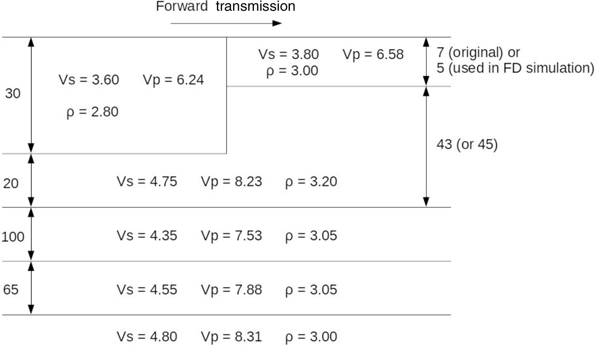
Figure 1 Schematic representation of “Model L”. Layer thicknesses are shown in km and units for velocity and density are km s⁻¹ and gm cc⁻¹ respectively. Note that crustal thickness on the right-hand side was originally 7 km but is modified to 5 km for comparisons with finite-difference results in this study. The layer thickness of 5 km facilitates the use of a 2.5 km FD grid, keeping the numerical problem computationally tractable (a 7 km thick layer would require a much finer FD grid spacing of 1 km).

Of the three methods included in this study, this is the one where mode conversions have actually been demonstrated in the published literature. Nonetheless, the method, hereafter referred to simply as the Alsop method, is included here for its remarkable simplicity.

a_r and b_t are obtained as solutions to the matrix equations

$$\begin{array}{}\text{(6)}& {\displaystyle }\begin{array}{rl}\mathbf{a}& ={\mathbf{C}}^{-\mathrm{1}}\mathbf{D}\\ \mathbf{b}& ={\left[{\mathbf{P}}^T\right]}_{\mathrm{1}}-{\mathbf{P}}^T\mathbf{a}\end{array},\end{array}$$

where

$$\begin{array}{}\text{(7)}& {\displaystyle }\begin{array}{rl}\mathbf{C}& =\mathbf{S}+{\mathbf{PT}}^T+{\mathbf{TP}}^T+{\mathbf{PVP}}^T\\ \mathbf{D}& =-{\left[\mathbf{S}\right]}_{\mathrm{1}}-{\left[{\mathbf{PT}}^T\right]}_{\mathrm{1}}+{\left[{\mathbf{TP}}^T\right]}_{\mathrm{1}}+{\left[{\mathbf{PVP}}^T\right]}_{\mathrm{1}}\end{array}\end{array}$$

and [X]_i denotes the ith column of any matrix X. The matrices P, S, T and V in the above equations are composed of the following integrals:

$$\begin{array}{}\text{(8)}& {\displaystyle }\begin{array}{rl}{P}_{ij}& ={\displaystyle \frac{k_i^{\left(\mathrm{1}\right)}}{\sqrt{N_i^{\left(\mathrm{1}\right)}{N}_j^{\left(\mathrm{2}\right)}}}}\underset{\mathrm{0}}{\overset{\mathrm{\infty }}{\int }}{\mathit{\mu }}^{\left(\mathrm{1}\right)}{\mathit{\varphi }}_i^{\mathrm{u}\left(\mathrm{1}\right)}{\mathit{\varphi }}_j^{\mathrm{u}\left(\mathrm{2}\right)}\mathrm{d}z\\ S_{ij}& ={\displaystyle \frac{\mathrm{1}}{\sqrt{N_i^{\left(\mathrm{1}\right)}{N}_j^{\left(\mathrm{1}\right)}}}}\underset{\mathrm{0}}{\overset{\mathrm{\infty }}{\int }}{\mathit{\varphi }}_i^{\mathrm{u}\left(\mathrm{1}\right)}{\mathit{\varphi }}_j^{\mathrm{u}\left(\mathrm{1}\right)}\mathrm{d}z\\ T_{ij}& ={\displaystyle \frac{\mathrm{1}}{\sqrt{N_i^{\left(\mathrm{1}\right)}{N}_j^{\left(\mathrm{2}\right)}}}}\underset{\mathrm{0}}{\overset{\mathrm{\infty }}{\int }}{\mathit{\varphi }}_i^{\mathrm{u}\left(\mathrm{1}\right)}{\mathit{\varphi }}_j^{\mathrm{u}\left(\mathrm{2}\right)}\mathrm{d}z\\ V_{ij}& ={\displaystyle \frac{\mathrm{1}}{\sqrt{N_i^{\left(\mathrm{2}\right)}{N}_j^{\left(\mathrm{2}\right)}}}}\underset{\mathrm{0}}{\overset{\mathrm{\infty }}{\int }}{\mathit{\varphi }}_i^{\mathrm{u}\left(\mathrm{2}\right)}{\mathit{\varphi }}_j^{\mathrm{u}\left(\mathrm{2}\right)}\mathrm{d}z.\end{array}\end{array}$$

To compute the transmission surface ratio (Y), we note that, for incident mode s and transmitted mode t, the ratio of transmitted to incident displacement is

$${\displaystyle \frac{B_{\mathrm{t}}{\mathit{\varphi }}_{\mathrm{t}}^{\left(\mathrm{2}\right)}}{A_{\mathrm{s}}{\mathit{\varphi }}_{\mathrm{s}}^{\left(\mathrm{1}\right)}}}=b_{\mathrm{t}}\times \left({\displaystyle \frac{{\mathit{\varphi }}_{\mathrm{t}}^{\left(\mathrm{2}\right)}}{{\mathit{\varphi }}_{\mathrm{s}}^{\left(\mathrm{1}\right)}}}\right)=b_{\mathrm{t}}\times \left({\displaystyle \frac{{\mathit{\varphi }}_{\mathrm{t}}^{\mathrm{u}\left(\mathrm{2}\right)}}{\sqrt{N_{\mathrm{t}}^{\left(\mathrm{2}\right)}}}}\times {\displaystyle \frac{\sqrt{N_{\mathrm{s}}^{\left(\mathrm{1}\right)}}}{{\mathit{\varphi }}_{\mathrm{s}}^{\mathrm{u}\left(\mathrm{1}\right)}}}\right).$$

In this study ϕ^u(1) and ϕ^u(2) have unit displacement at the surface; therefore

$$\begin{array}{}\text{(9)}& Y_{\mathrm{st}}=b_{\mathrm{t}}\times \sqrt{{\displaystyle \frac{N_{\mathrm{s}}^{\left(\mathrm{1}\right)}}{N_{\mathrm{t}}^{\left(\mathrm{2}\right)}}}}.\end{array}$$

Figure 2 Transmission surface ratio obtained by the GAl method (solid lines) and GF method (dashed lines with circles), for an incident Love wave fundamental mode (mode 0) propagating through the original model L in the forward direction (a) and backward direction (b). The SWRT package accounts for all the modes that exist in a given medium at a given frequency; note that in this figure the highest modes, where they exist, have negligible amplitudes. Here and in all following figures, the various surface wave modes are labelled according to their mode number, starting from 0 for the fundamental and increasing successively for each higher mode.

2.2 Body wave method of Gregersen and Alsop (1974)

This method is founded on representing the field of surface waves as a superposition of plane homogeneous and inhomogeneous body waves. Body wave reflection and transmission coefficients are computed over the vertical interface to obtain outgoing stresses and displacements on the interface. This outgoing stress-displacement system is regarded as the source of outgoing surface waves, whose amplitudes are computed via its projection onto the outgoing surface wave eigenfunctions. In this study the method, hereafter referred to as the GAl method, is implemented, as follows for Love waves:

1. SH wave reflection and transmission coefficients over the vertical contact are calculated using the phase velocity of medium 1.

   Elementary formulae are used for the SH reflection and transmission coefficients (Γ_R and Γ_T). The textbook expressions (e.g. Lay and Wallace, 1995, p. 102)

   $$\begin{array}{}\text{(10)}& \begin{array}{r}{\mathrm{\Gamma }}_R={\displaystyle \frac{{\mathit{\rho }}_{\mathrm{1}}{\mathit{\beta }}_{\mathrm{1}}\cos {\mathit{\theta }}_i-{\mathit{\rho }}_{\mathrm{2}}{\mathit{\beta }}_{\mathrm{2}}\cos {\mathit{\theta }}_{\mathrm{t}}}{{\mathit{\rho }}_{\mathrm{1}}{\mathit{\beta }}_{\mathrm{1}}\cos {\mathit{\theta }}_i+{\mathit{\rho }}_{\mathrm{2}}{\mathit{\beta }}_{\mathrm{2}}\cos {\mathit{\theta }}_{\mathrm{t}}}}\\ {\mathrm{\Gamma }}_T={\displaystyle \frac{\mathrm{2}{\mathit{\rho }}_{\mathrm{1}}{\mathit{\beta }}_{\mathrm{1}}\cos {\mathit{\theta }}_i}{{\mathit{\rho }}_{\mathrm{1}}{\mathit{\beta }}_{\mathrm{1}}\cos {\mathit{\theta }}_i+{\mathit{\rho }}_{\mathrm{2}}{\mathit{\beta }}_{\mathrm{2}}\cos {\mathit{\theta }}_{\mathrm{t}}}}\end{array}\end{array}$$

   for plane SH rays at an interface between two solid media (the symbols have their usual meanings) are rewritten in terms of phase velocity because cos θ_i and cos θ_t can be rewritten (by Snell's law) in terms of the phase velocity c₁ of the incidence-side medium (Keilis-Borok, 1989):

   $$\begin{array}{}\text{(11)}& {\displaystyle }\begin{array}{rl}{\mathrm{\Gamma }}_R& ={\displaystyle \frac{{\mathit{\mu }}_{\mathrm{1}}/c_{\mathrm{1}}-{\mathit{\mu }}_{\mathrm{2}}\sqrt{\mathrm{1}/{{\mathit{\beta }}_{\mathrm{2}}}^{\mathrm{2}}-\mathrm{1}/{{\mathit{\beta }}_{\mathrm{1}}}^{\mathrm{2}}+\mathrm{1}/{c_{\mathrm{1}}}^{\mathrm{2}}}}{{\mathit{\mu }}_{\mathrm{1}}/c_{\mathrm{1}}+{\mathit{\mu }}_{\mathrm{2}}\sqrt{\mathrm{1}/{{\mathit{\beta }}_{\mathrm{2}}}^{\mathrm{2}}-\mathrm{1}/{{\mathit{\beta }}_{\mathrm{1}}}^{\mathrm{2}}+\mathrm{1}/{c_{\mathrm{1}}}^{\mathrm{2}}}}}\\ {\mathrm{\Gamma }}_T& =\mathrm{1}+{\mathrm{\Gamma }}_R.\end{array}\end{array}$$

   These equations are applied individually to each section of the vertical interface, i.e. each layered contact (there is really a layer index in addition to the medium index in Eqs. 10 and 11 but it has been left out for notational convenience) to obtain a vector of body wave coefficients over the entire vertical interface.

2. Outgoing stresses and displacements as a function of depth over the vertical interface are calculated using the eigenfunction of the incident Love wave mode and the SH reflection/transmission coefficients.

3. Coupling between the interface stress-displacement system and the eigenfunctions of outgoing Love waves (eigenfunctions of medium 1 for reflection, those of medium 2 for transmission) is calculated by means of the Herrera (1964) scalar product.

Since Herrera's scalar product may be computed for any two stress-displacement vectors S^m and Sⁿ, this method uses Love–Love and SH–Love systems. In the former case Eq. (1) defines the orthonormalization of Love wave eigenfunctions; in the latter it yields the coupling coefficient for the GAl method. This means that when the surface wave modes are normalized by Eq. (1), the coupling computed (by the left-hand side of the same) between any stress-displacement system and a surface wave mode is the amplitude generated of that normalized surface wave mode.

So if S_R and S_T are the SH stress-displacement vectors on the interface computed in step 2 of the algorithm, Love wave reflection and transmission coefficients are given by (S_R,ϕ⁽¹⁾) and (S_T,ϕ⁽²⁾). Therefore in this study they are computed as

$$\begin{array}{}\text{(12)}& {\displaystyle }\begin{array}{rl}{a}_{\mathrm{r}}& ={\displaystyle \frac{(S_R,{\mathit{\varphi }}_{\mathrm{r}}^{\mathrm{u}\left(\mathrm{1}\right)})}{\sqrt{N_{\mathrm{s}}^{\left(\mathrm{1}\right)}{N}_{\mathrm{r}}^{\left(\mathrm{1}\right)}}}}\\ b_{\mathrm{t}}& ={\displaystyle \frac{(S_T,{\mathit{\varphi }}_{\mathrm{t}}^{\mathrm{u}\left(\mathrm{2}\right)})}{\sqrt{N_{\mathrm{s}}^{\left(\mathrm{1}\right)}{N}_{\mathrm{t}}^{\left(\mathrm{2}\right)}}}}.\end{array}\end{array}$$

In the above expressions the norms N have the usual definition given by Eq. (4), whilst the numerators are similarly evaluated using μ and k values corresponding to the incidence-side medium for a_r and to the transmission-side medium for b_t. Finally, as with the Alsop method, transmission surface ratio is given by

$$\begin{array}{}\text{(13)}& Y=b\times \sqrt{{\displaystyle \frac{N^{\left(\mathrm{1}\right)}}{N^{\left(\mathrm{2}\right)}}}}={\displaystyle \frac{(S_T,{\mathit{\varphi }}^{\left(\mathrm{2}\right)})}{N^{\left(\mathrm{2}\right)}}}.\end{array}$$

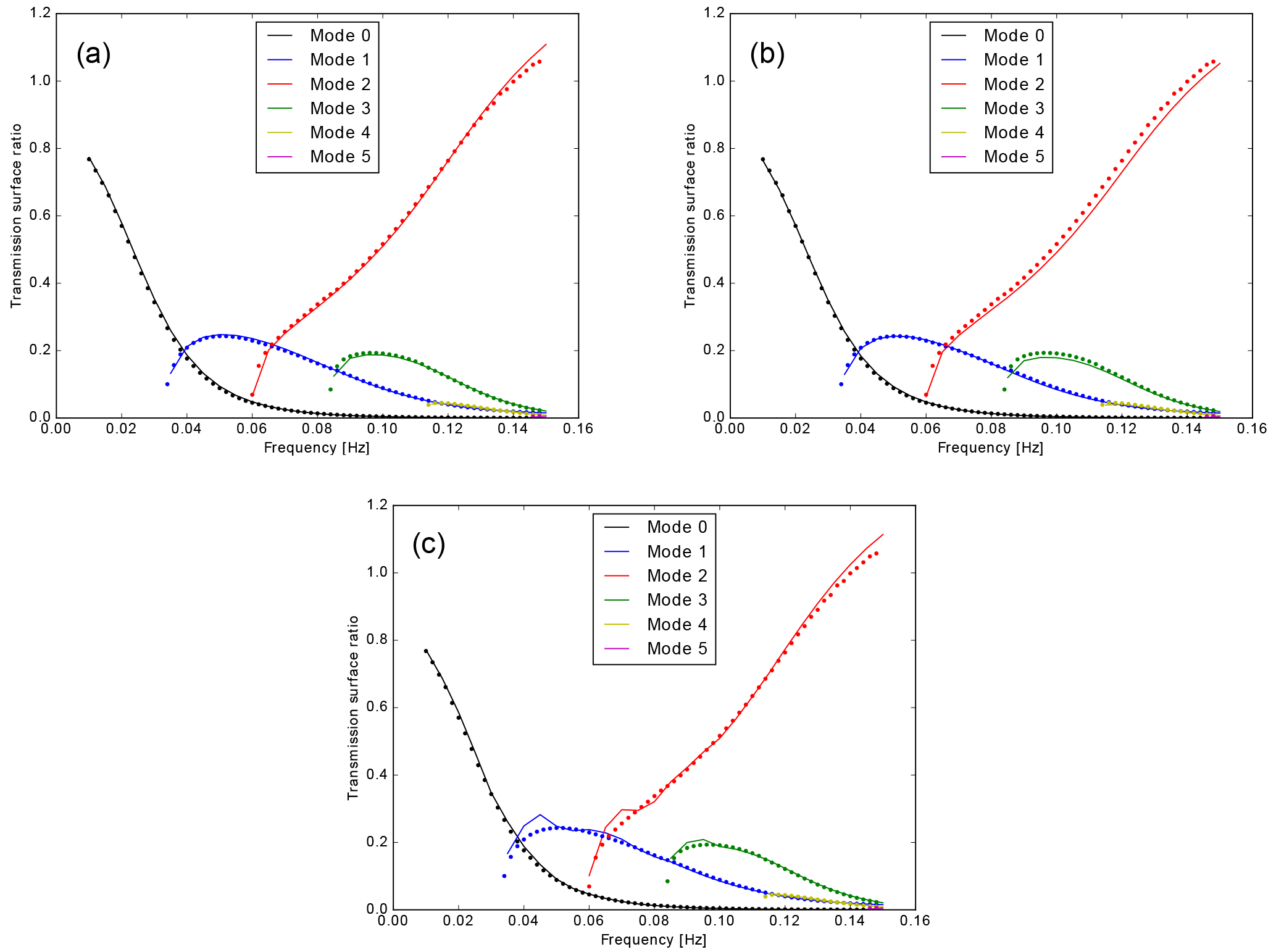
Figure 3 Transmission surface ratios obtained from the SWRT code (solid lines) and FD calculations (dots), for an incident Love wave fundamental mode propagating through the modified model L in the forward direction. (a) Using the GAl method; (b) using the GF method; (c) using the Alsop method. Note that the FD results are the same in all three plots. The last plot (c) is shown to highlight the weaker performance of the Alsop method (at the low-frequency end for the first and second higher modes), compared to the two methods which are the focus of this paper.

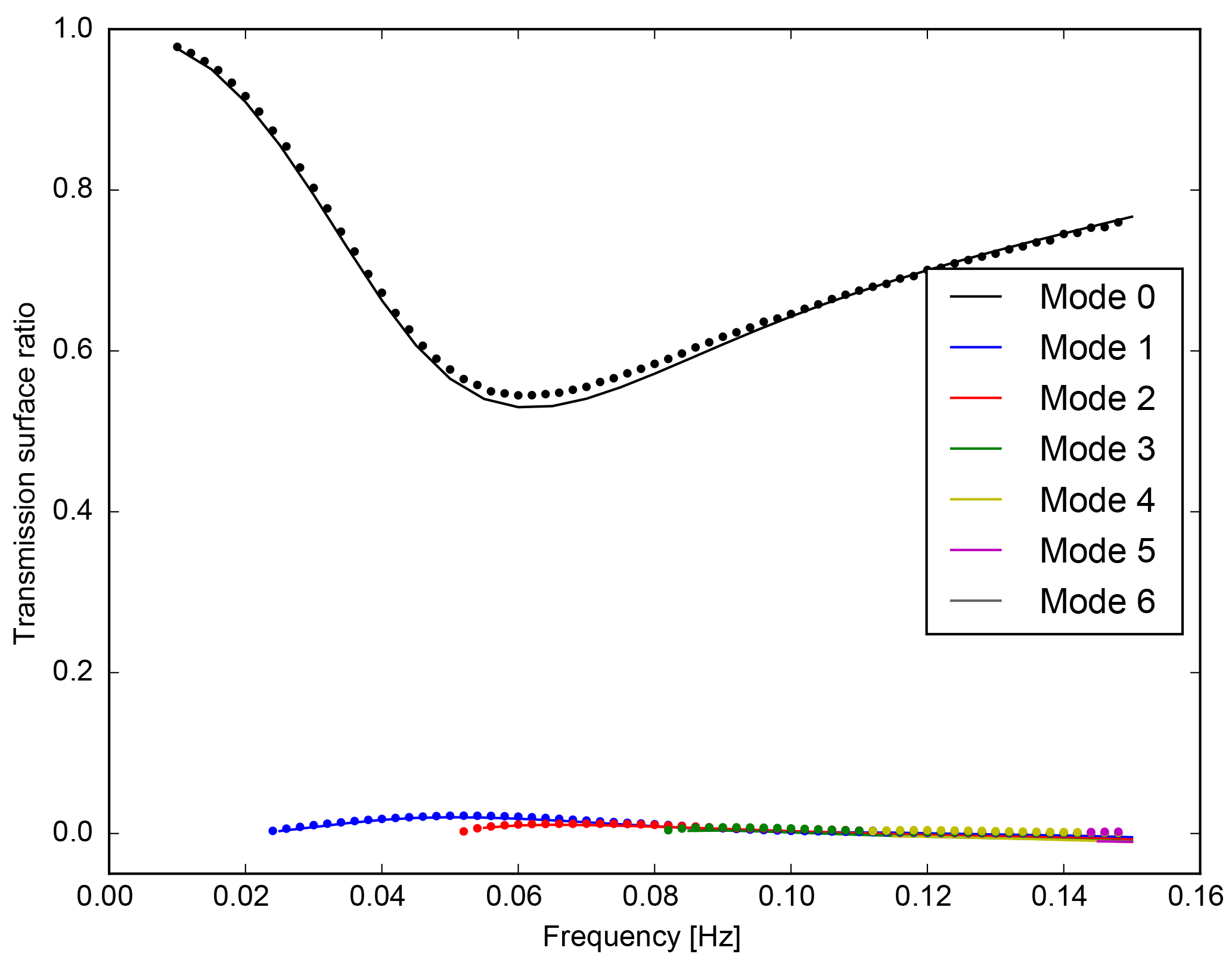
Figure 4 Transmission surface ratio obtained by the GF method (solid lines) and FD calculations (dots), for an incident Rayleigh wave fundamental mode propagating through model L in the forward direction. Note that the conversion to higher modes is much weaker than in the Love wave case, but the SWRT result is in good agreement with the FD result.

2.3 Green's function method of Its and Yanovskaya (1985)

This method, hereafter referred to as the GF method, has been implemented in SWRT for both Love and Rayleigh waves. We follow the algorithm of Its and Yanovskaya (1985, hereafter ItsYan85), who obtained the coupled system of equations:

$$\begin{array}{}\text{(14)}& {\displaystyle }\begin{array}{rl}{a}_{\mathrm{r}}& =-\sum _{\mathrm{t}}{b}_{\mathrm{t}}{P}_{\mathrm{rt}}\\ b_{\mathrm{t}}& =S_{\mathrm{st}}^{*}+\sum _{\mathrm{r}}{a}_{\mathrm{r}}{P}_{\mathrm{rt}}^{*},\end{array}\end{array}$$

where P_rt and S_st are the coupling integrals

$$\begin{array}{}\text{(15)}& {\displaystyle }\begin{array}{rl}{P}_{\mathrm{rt}}& ={\displaystyle \frac{\mathrm{1}}{J_{\mathrm{r}}^{\left(\mathrm{1}\right)}}}\underset{\mathrm{0}}{\overset{\mathrm{\infty }}{\int }}\left[{\mathit{\sigma }}_{\mathrm{r}}^{\left(\mathrm{1}\right)}\cdot {\mathit{u}}_{\mathrm{t}}^{\left(\mathrm{2}\right)}-{\mathit{u}}_{\mathrm{r}}^{\left(\mathrm{1}\right)}\cdot {\mathit{\sigma }}_{\mathrm{t}}^{\left(\mathrm{2}\right)}\right]\mathrm{d}z\\ S_{\mathrm{st}}& ={\displaystyle \frac{\mathrm{1}}{J_{\mathrm{t}}^{\left(\mathrm{2}\right)}}}\underset{\mathrm{0}}{\overset{\mathrm{\infty }}{\int }}\left[{\mathit{\sigma }}_{\mathrm{s}}^{\left(\mathrm{1}\right)*}\cdot {\mathit{u}}_{\mathrm{t}}^{\left(\mathrm{2}\right)}-{\mathit{u}}_{\mathrm{s}}^{\left(\mathrm{1}\right)*}\cdot {\mathit{\sigma }}_{\mathrm{t}}^{\left(\mathrm{2}\right)}\right]\mathrm{d}z,\end{array}\end{array}$$

where u and σ are the displacement and traction vectors on the vertical plane of discontinuity, and J_m=2H_m. Using the appropriate u and σ in Eq. (15) leads to explicit expressions for the Love and Rayleigh cases.

Building the system of equations

1. Love waves — these expressions are easily derived as there is only one component of displacement and traction relevant for Eq. (15). The norm J_m reduces to 2i×N_m and for eigenfunctions normalized by Eq. (3), $J_{\mathrm{r}}^{\left(\mathrm{1}\right)}=J_{\mathrm{t}}^{\left(\mathrm{2}\right)}=\mathrm{2}i$, leading to factors of 1∕2 outside the integrals in Eq. (15). In this study, working with ϕ^u, P and S are computed as

   $$\begin{array}{}\text{(16)}& {\displaystyle }\begin{array}{rl}{P}_{\mathrm{rt}}& ={\displaystyle \frac{\mathrm{1}}{\mathrm{2}\sqrt{N_r^{\left(\mathrm{1}\right)}{N}_{\mathrm{t}}^{\left(\mathrm{2}\right)}}}}\left[k_{\mathrm{t}}^{\left(\mathrm{2}\right)}\underset{\mathrm{0}}{\overset{\mathrm{\infty }}{\int }}{\mathit{\mu }}^{\left(\mathrm{2}\right)}{\mathit{\varphi }}_{\mathrm{r}}^{\mathrm{u}\left(\mathrm{1}\right)}{\mathit{\varphi }}_{\mathrm{t}}^{\mathrm{u}\left(\mathrm{2}\right)}\mathrm{d}z\right.\\ & \left.-k_{\mathrm{r}}^{\left(\mathrm{1}\right)}\underset{\mathrm{0}}{\overset{\mathrm{\infty }}{\int }}{\mathit{\mu }}^{\left(\mathrm{1}\right)}{\mathit{\varphi }}_{\mathrm{r}}^{\mathrm{u}\left(\mathrm{1}\right)}{\mathit{\varphi }}_{\mathrm{t}}^{\mathrm{u}\left(\mathrm{2}\right)}\mathrm{d}z\right]\\ S_{\mathrm{st}}& ={\displaystyle \frac{\mathrm{1}}{\mathrm{2}\sqrt{N_s^{\left(\mathrm{1}\right)}{N}_{\mathrm{t}}^{\left(\mathrm{2}\right)}}}}\left[k_{\mathrm{t}}^{\left(\mathrm{2}\right)}\underset{\mathrm{0}}{\overset{\mathrm{\infty }}{\int }}{\mathit{\mu }}^{\left(\mathrm{2}\right)}{\mathit{\varphi }}_{\mathrm{s}}^{\mathrm{u}\left(\mathrm{1}\right)}{\mathit{\varphi }}_{\mathrm{t}}^{\mathrm{u}\left(\mathrm{2}\right)}\mathrm{d}z\right.\\ & \left.+k_{\mathrm{s}}^{\left(\mathrm{1}\right)}\underset{\mathrm{0}}{\overset{\mathrm{\infty }}{\int }}{\mathit{\mu }}^{\left(\mathrm{1}\right)}{\mathit{\varphi }}_{\mathrm{s}}^{\mathrm{u}\left(\mathrm{1}\right)}{\mathit{\varphi }}_{\mathrm{t}}^{\mathrm{u}\left(\mathrm{2}\right)}\mathrm{d}z\right].\end{array}\end{array}$$

2. Rayleigh waves — the expressions have been derived by Keilis-Borok (1989), using a nomenclature similar to that of Aki and Richards (2002) for the stress-displacement vector, although with a sign error in one of the terms. The expressions used in this study are different, because they are based on the stress-displacement vector as defined by Gomberg and Masters (1988). The stress-displacement vector is ${\mathit{\beta }}_{\mathrm{1}},{\mathit{\beta }}_{\mathrm{2}},{\mathit{\beta }}_{\mathrm{3}},{\mathit{\beta }}_{\mathrm{4}}$, and in terms of these quantities the coupling integrals are (Appendix Appendix A)

   $$\begin{array}{}\text{(17)}& {\displaystyle }\begin{array}{rl}{P}_{\mathrm{rt}}& ={\displaystyle \frac{i}{\mathit{\omega }{J}_{\mathrm{r}}^{\left(\mathrm{1}\right)}}}\underset{\mathrm{0}}{\overset{\mathrm{\infty }}{\int }}\left[{\mathit{\psi }}_{xx}^{\mathrm{t}\left(\mathrm{2}\right)}{\mathit{\beta }}_{\mathrm{2}}^{\mathrm{r}\left(\mathrm{1}\right)}-{\mathit{\psi }}_{xx}^{\mathrm{r}\left(\mathrm{1}\right)}{\mathit{\beta }}_{\mathrm{2}}^{\mathrm{t}\left(\mathrm{2}\right)}+{\mathit{\beta }}_{\mathrm{1}}^{\mathrm{r}\left(\mathrm{1}\right)}{\mathit{\beta }}_{\mathrm{4}}^{\mathrm{t}\left(\mathrm{2}\right)}\right.\\ & \left.-{\mathit{\beta }}_{\mathrm{1}}^{\mathrm{t}\left(\mathrm{2}\right)}{\mathit{\beta }}_{\mathrm{4}}^{\mathrm{r}\left(\mathrm{1}\right)}\right]\mathrm{d}z\\ S_{\mathrm{st}}& ={\displaystyle \frac{i}{\mathit{\omega }{J}_{\mathrm{t}}^{\left(\mathrm{2}\right)}}}\underset{\mathrm{0}}{\overset{\mathrm{\infty }}{\int }}\left[{\mathit{\psi }}_{xx}^{\mathrm{s}\left(\mathrm{1}\right)}{\mathit{\beta }}_{\mathrm{2}}^{\mathrm{t}\left(\mathrm{2}\right)}+{\mathit{\psi }}_{xx}^{\mathrm{t}\left(\mathrm{2}\right)}{\mathit{\beta }}_{\mathrm{2}}^{\mathrm{s}\left(\mathrm{1}\right)}-{\mathit{\beta }}_{\mathrm{4}}^{\mathrm{s}\left(\mathrm{1}\right)}{\mathit{\beta }}_{\mathrm{1}}^{\mathrm{t}\left(\mathrm{2}\right)}\right.\\ & \left.-{\mathit{\beta }}_{\mathrm{4}}^{\mathrm{t}\left(\mathrm{2}\right)}{\mathit{\beta }}_{\mathrm{1}}^{\mathrm{s}\left(\mathrm{1}\right)}\right]\mathrm{d}z,\end{array}\end{array}$$

   with the norm given by

   $$\begin{array}{}\text{(18)}& J_m={\displaystyle \frac{\mathrm{2}i}{\mathit{\omega }}}\underset{\mathrm{0}}{\overset{\mathrm{\infty }}{\int }}\left[{\mathit{\psi }}_{xx}^m{\mathit{\beta }}_{\mathrm{2}}^m-{\mathit{\beta }}_{\mathrm{4}}^m{\mathit{\beta }}_{\mathrm{1}}^m\right]\mathrm{d}z\end{array}$$

   and ψ_xx defined by Eq. (A2). Note that in the Rayleigh case, the eigenfunctions themselves have subscripts 1–4; these should not be confused with the medium indices 1–2 which are shown as superscripts and in parentheses.

Solving the system of equations

In our implementation P_rt and S_st are both real-valued, so the system of Eq. (14) is solved as

$$\begin{array}{}\text{(19)}& {\displaystyle }\begin{array}{rl}\sum _{t=\mathrm{0}}^T{P}_{\mathrm{rt}}{b}_{\mathrm{t}}+a_{\mathrm{r}}& =\mathrm{0}\\ b_{\mathrm{t}}-\sum _{r=\mathrm{0}}^R{P}_{\mathrm{rt}}{a}_{\mathrm{r}}& =S_{\mathrm{st}}\end{array},\end{array}$$

where R and T are the highest mode numbers that exist in the incidence-side and transmission-side media respectively at the given frequency. Equation (14) is easily recognized as a matrix equation of the form Cx=d:

$$\begin{array}{ll}{\displaystyle }& {\displaystyle }\left[\begin{array}{cccccccc}{P}_{\mathrm{00}}& P_{\mathrm{01}}& \mathrm{\cdots }& P_{\mathrm{0}T}& \mathrm{1}& \mathrm{0}& \mathrm{\cdots }& \mathrm{0}\\ \mathrm{⋮}& \mathrm{\ddots }& \mathrm{\ddots }& & \mathrm{0}& \mathrm{\ddots }& \mathrm{\ddots }& \\ P_{R\mathrm{0}}& \mathrm{\cdots }& & P_{RT}& \mathrm{0}& \mathrm{\cdots }& & \mathrm{1}\\ \mathrm{1}& \mathrm{0}& \mathrm{\cdots }& \mathrm{0}& -P_{\mathrm{00}}& -P_{\mathrm{10}}& \mathrm{\cdots }& -P_{R\mathrm{0}}\\ \mathrm{0}& \mathrm{\ddots }& \mathrm{\ddots }& & \mathrm{⋮}& \mathrm{\ddots }& \mathrm{\ddots }\\ \mathrm{0}& \mathrm{\cdots }& & \mathrm{1}& -P_{\mathrm{0}T}& \mathrm{\cdots }& & -P_{RT}\end{array}\right]\\ \text{(20)}& {\displaystyle }& {\displaystyle }\left[\begin{array}{c}{b}_{\mathrm{0}}\\ \mathrm{⋮}\\ b_T\\ a_{\mathrm{0}}\\ \mathrm{⋮}\\ a_R\end{array}\right]=\left[\begin{array}{c}\mathrm{0}\\ \mathrm{⋮}\\ \mathrm{0}\\ S_{s\mathrm{0}}\\ \mathrm{⋮}\\ S_{sT}\end{array}\right],\end{array}$$

which is a square system of equations of size $(T+R+\mathrm{2})$. In general R≠T and this can lead to cumbersome code because of the variability in the declaration of array sizes. However SWRT achieves efficiency with a single declaration regardless of the relationship between R and T. In the special case when $R=T\text{ (}=M-\mathrm{1}\text{, say})$, the coefficient matrix of this system is itself composed of square sub-matrices:

$$\begin{array}{}\text{(21)}& \mathbf{C}=\left[\begin{array}{cc}{\mathbf{P}}_M& {\mathbf{I}}_M\\ {\mathbf{I}}_M& -{{\mathbf{P}}^{\mathbf{T}}}_M\end{array}\right].\end{array}$$

Figure 5 Schematic representation of the model of Sato (1961). Units of layer parameters are the same as in Fig. 1.

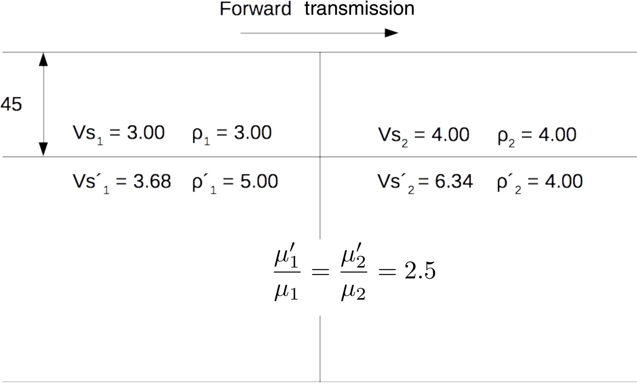
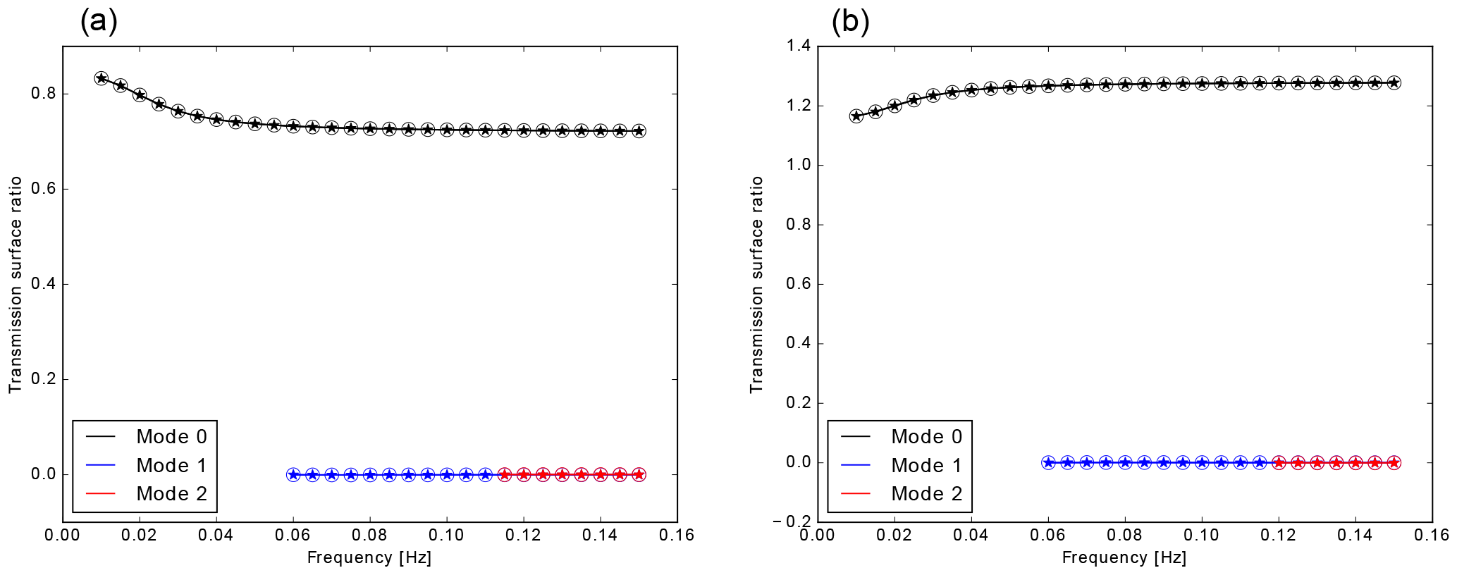
Figure 6 Transmission surface ratios for an incident Love wave fundamental mode propagating in the forward direction (a) and backward direction (b) in the Sato model. Shown are results from the GAl method (solid lines), the GF method (circles) and the method of Alsop (stars). Even though higher modes exist in the model at the frequencies considered and SWRT by default computes coupling to all modes that exist at any given frequency, all three methods exactly predict that there is no mode conversion.

Finally, we note that in computing the transmission surface ratio (Y), there is a subtle difference between the Love and Rayleigh cases. In the Love wave case, the appearance of the normalization factors for both media outside the brackets in Eq. (16) ensures that the a_r and b_t obtained from Eq. (19) are defined with respect to eigenfunctions normalized according to Eq. (3); therefore, as before, $Y_{\mathrm{st}}=b_{\mathrm{t}}\times \sqrt{N_{\mathrm{s}}^{\left(\mathrm{1}\right)}/N_{\mathrm{t}}^{\left(\mathrm{2}\right)}}$. However the same is not true of the Rayleigh case – the implementation Eq. (17) ensures that the reflection and transmission coefficients obtained from Eq. (19) are in fact defined with respect to the eigenfunctions β, which have unit surface displacement. Hence, in the Rayleigh case, Y_st=b_t.

The three methods described in this section are each implemented as Python programs in the SWRT code. The only inputs these programs require are the eigenfunctions for the two media on either side of the lateral discontinuity and the depths of horizontal interfaces in these media. The programs have been tested using published results in the literature (Appendix Appendix B); in the following section we focus on results from the latter two methods, which are incomplete in the published literature.

3 Demonstration of results

We use a single model to demonstrate the capabilities of the GAl and GF methods. This is a model of an ocean–continent boundary known as “model L” (Fig. 1), and was used by both Gregersen and Alsop (1974, hereafter GregAl74) and ItsYan85. Both of these studies considered the propagation of a Love wave fundamental mode through this model, in both directions and over a range of frequencies in which a number of higher modes exist on the transmission side. However both studies have shown only the transmission of the fundamental mode, with no mention of any conversion to higher modes. Using the SWRT code, we find that considering periods as short as ∼ 7 s, there is significant conversion of the fundamental mode to up to the fourth overtone, for propagation in either direction (Fig. 2). Concurrently, the fundamental mode result obtained from SWRT is in good agreement with the published results (see Appendix Appendix B).

To validate our results of transmission to multiple higher modes, we compare the SWRT result with results from finite-difference (FD) simulations. The FD simulations are performed using the method of Roecker et al. (2010) duly adapted for teleseismic surface wave modelling. However for the FD comparison, model L is modified slightly in that the crustal thickness on the oceanic side is taken as 5 km rather than 7 km (see Fig. 1). In the rest of this section, all “model L” references imply this modified version.

Figure 3 shows excellent agreement between the SWRT results (GAl and GF methods) and FD results for Love waves in model L. Only forward propagation is considered. The corresponding Rayleigh case is shown in Fig. 4.

Figures 2–4 represent the core contribution of this study. The reader is reminded that model L has only been used as a demo example in this study. The published literature does not contain any examples of mode conversions modelled by the GAl method or the GF method, whilst the SWRT code provides complete solutions (with coupling to all possible modes) in any model containing a single vertical contact between two laterally homogeneous media. To emphasize this point as well as the general accuracy of the SWRT code, we provide a second demonstration using the model of Sato (1961). This is a unique model (Fig. 5) in which the Love wave reflection and transmission problem has an exact solution – the Love wave eigenfunctions on both sides of the discontinuity have the same shape; therefore, boundary conditions on either side of the discontinuity can be exactly satisfied by these eigenfunctions, therefore there is no mode conversion in this model, in either direction. Figure 6 demonstrates this with SWRT results.

4 Discussion and conclusions

This paper has described the author's SWRT code and used it to demonstrate cross-branch mode coupling, of both Love and Rayleigh waves, in simple 2-D models for which previously published results showed only self coupling. SWRT provides a consolidated implementation of sophisticated algorithms by previous authors, which is fully capable of modelling mode conversions arising from normal incidence at a single lateral discontinuity. These algorithms are more accurate than that of Alsop66, whose ability to model mode conversion has been known since the original author's work.

We conclude with remarks on the transferability and flexibility of the SWRT code. Whilst the code has been written to work with a specific format of input file (containing the surface wave eigenfunctions), it is modular with respect to file input: the eigenfunction-reading module of SWRT, which has nothing to do with the algorithms discussed in this paper, can simply be replaced in order to adapt the code to differently formatted input files. Possible additional work may be to modify the expressions for the coupling coefficients in the main programs, depending on the theoretical definitions of the eigenfunctions. As a further comment on flexibility, there is no restriction on the type of normalization that the input eigenfunctions must obey; only the expressions for surface ratios will need modification if the eigenfunctions are not normalized to unit surface displacement. Finally, whilst results have been presented in this paper only for the case of an incident fundamental mode, application of SWRT to the case of arbitrary mode number being incident can be trivially achieved.

Appendix A: Rayleigh wave expressions in the Green's function method

The Rayleigh wave stress-displacement vector defined by Gomberg and Masters (1988) is $\mathit{\beta }=\mathit{\{}{\mathit{\beta }}_{\mathrm{1}},{\mathit{\beta }}_{\mathrm{2}},{\mathit{\beta }}_{\mathrm{3}},{\mathit{\beta }}_{\mathrm{4}}\mathit{\}}$, the four components being proportional to $u_z,u_x,{\mathit{\sigma }}_{zz}$ and σ_xz respectively:

$$\begin{array}{}\text{(A1)}& {\displaystyle }\begin{array}{rl}{u}_x& =\left({\displaystyle \frac{-{\mathit{\beta }}_{\mathrm{2}}}{\mathit{\omega }}}\right)e^{i(kx-\mathit{\omega }t)}\\ u_z& =i\left({\displaystyle \frac{{\mathit{\beta }}_{\mathrm{1}}}{\mathit{\omega }}}\right)e^{i(kx-\mathit{\omega }t)}\\ {\mathit{\sigma }}_{xz}& =-{\mathit{\beta }}_{\mathrm{4}}{e}^{i(kx-\mathit{\omega }t)}\\ {\mathit{\sigma }}_{zz}& =i{\mathit{\beta }}_{\mathrm{3}}{e}^{i(kx-\mathit{\omega }t)}\end{array}.\end{array}$$

For the type of problem under consideration, with the plane interface being normal to the x direction, the required components of traction are σ_xz and σ_xx. The latter can be written in terms of β₁ and β₂ (with the phase factor omitted for convenience):

$$\begin{array}{ll}{\displaystyle }{\mathit{\sigma }}_{xx}& {\displaystyle }=\mathit{\lambda }\left[{\displaystyle \frac{\partial u_x}{\partial x}}+{\displaystyle \frac{\partial u_z}{\partial z}}\right]+\mathrm{2}\mathit{\mu }{\displaystyle \frac{\partial u_x}{\partial x}}\\ \text{(A2)}& {\displaystyle }& {\displaystyle }={\displaystyle \frac{i}{\mathit{\omega }}}\left[\mathit{\lambda }{\displaystyle \frac{d{\mathit{\beta }}_{\mathrm{1}}}{\mathrm{d}z}}-k(\mathit{\lambda }+\mathrm{2}\mathit{\mu }){\mathit{\beta }}_{\mathrm{2}}\right]=i{\mathit{\psi }}_{xx}.\end{array}$$

The first requirement is to obtain an expression for the scalar product J_mn=2H_mn. Using Eq. (A2) and the first three parts of Eq. (A1),

$$\begin{array}{}\text{(A3)}& {\displaystyle }\begin{array}{rl}{J}_{mn}& =\underset{\mathrm{0}}{\overset{\mathrm{\infty }}{\int }}\left({\mathit{\sigma }}_m^{*}\cdot {\mathit{u}}_n-{\mathit{u}}_m^{*}\cdot {\mathit{\sigma }}_n\right)\mathrm{d}z\\ & =\underset{\mathrm{0}}{\overset{\mathrm{\infty }}{\int }}\left[\left(-i{\mathit{\psi }}_{xx}^m\widehat{x}-{\mathit{\beta }}_{\mathrm{4}}^m\widehat{z}\right)\left(-{\displaystyle \frac{{\mathit{\beta }}_{\mathrm{2}}^n}{\mathit{\omega }}}\widehat{x}+{\displaystyle \frac{i{\mathit{\beta }}_{\mathrm{1}}^n}{\mathit{\omega }}}\widehat{z}\right)\right.\\ & \left.-\left(-{\displaystyle \frac{{\mathit{\beta }}_{\mathrm{2}}^m}{\mathit{\omega }}}\widehat{x}-{\displaystyle \frac{i{\mathit{\beta }}_{\mathrm{1}}^m}{\mathit{\omega }}}\widehat{z}\right)\left(i{\mathit{\psi }}_{xx}^n\widehat{x}-{\mathit{\beta }}_{\mathrm{4}}^n\widehat{z}\right)\right]\mathrm{d}z\\ & ={\displaystyle \frac{i}{\mathit{\omega }}}\underset{\mathrm{0}}{\overset{\mathrm{\infty }}{\int }}\left[{\mathit{\psi }}_{xx}^m{\mathit{\beta }}_{\mathrm{2}}^n+{\mathit{\psi }}_{xx}^n{\mathit{\beta }}_{\mathrm{2}}^m-{\mathit{\beta }}_{\mathrm{4}}^m{\mathit{\beta }}_{\mathrm{1}}^n-{\mathit{\beta }}_{\mathrm{4}}^n{\mathit{\beta }}_{\mathrm{1}}^m\right]\mathrm{d}z\end{array}.\end{array}$$

So the norm required in Eq. (15) is

$$J_m={\displaystyle \frac{\mathrm{2}i}{\mathit{\omega }}}\underset{\mathrm{0}}{\overset{\mathrm{\infty }}{\int }}\left[{\mathit{\psi }}_{xx}^m{\mathit{\beta }}_{\mathrm{2}}^m-{\mathit{\beta }}_{\mathrm{4}}^m{\mathit{\beta }}_{\mathrm{1}}^m\right]\mathrm{d}z.$$

Similarly the expressions for the coupling integrals P_rt and S_st can be evaluated using Eq. (15) and the result is Eq. (17) of the main text.

Appendix B: Comparison with published results

B1 The GAl method

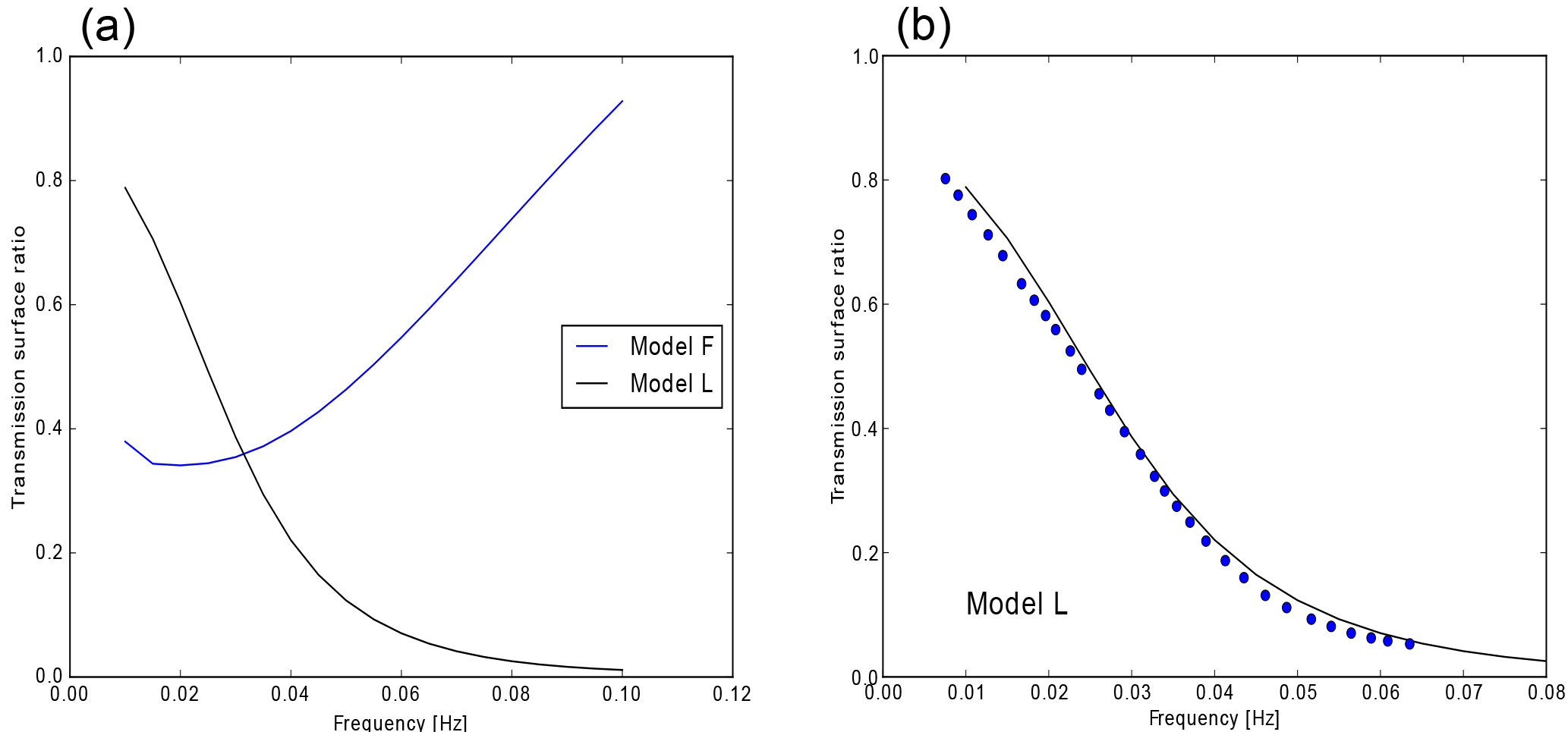
Figure B1 (a) Fundamental mode Love wave surface transmission ratios for models “F” and “L”, which were used by GregAl74 as well as ItsYan85. To be compared with Fig. 5 of ItsYan85. (b) SWRT result for model L (solid line, same as in a) compared with values obtained by manually digitizing Fig. 5 of ItsYan85 (circles).

Figure B1 provides a comparison of SWRT results with published results, for the GAl method (Love wave case).

B2 The GF method

Figure B2 provides a comparison of SWRT results with published results, for the GF method (Rayleigh wave case).

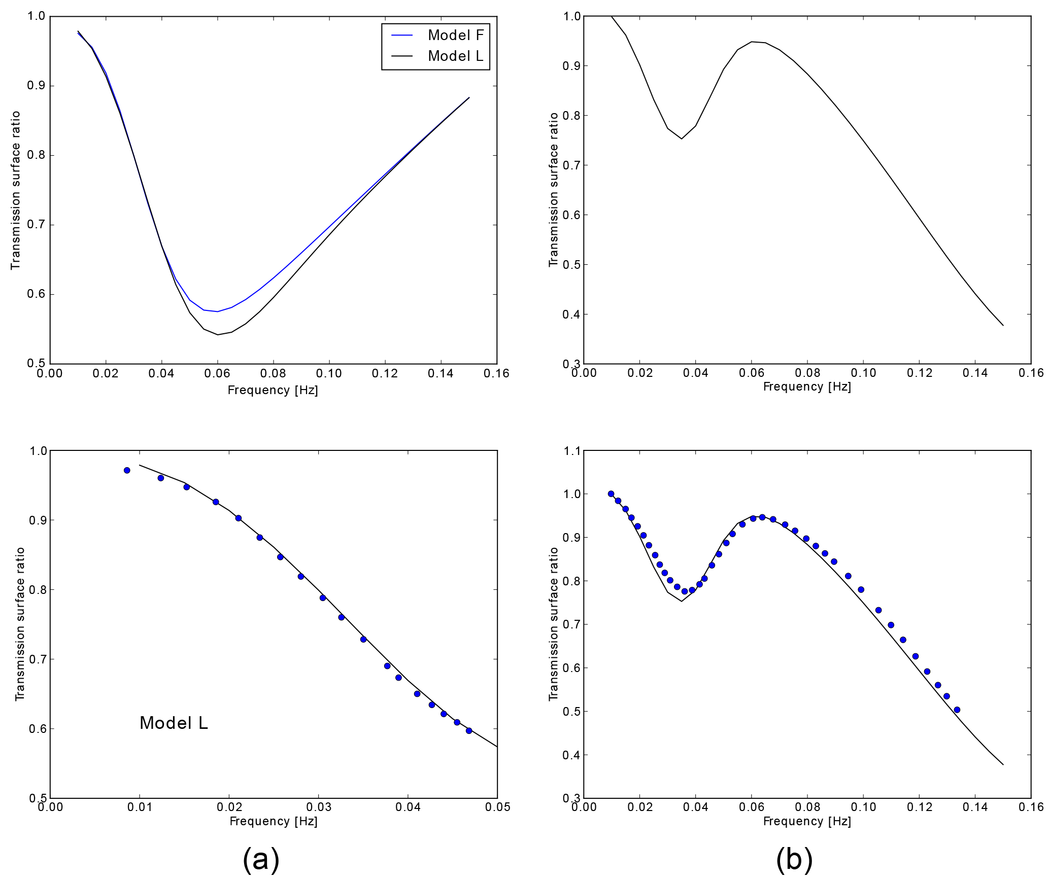
Figure B2 Rayleigh wave fundamental mode transmission surface ratios for two types of models taken from ItsYan85: (a) models “F” and “L”, same as for Fig. B1, and (b) the deep fault model, Fig. 10 of ItsYan85. In both cases the top panel shows the SWRT results; the bottom panel compares these (lines) with manually digitized values (circles) obtained from Figs. 9 and 11 – for (a) and (b) respectively – of ItsYan85.

B3 The Alsop method

Figure B3 shows SWRT results computed by the Alsop method, presented in the same format as Alsop66 for a visual comparison.

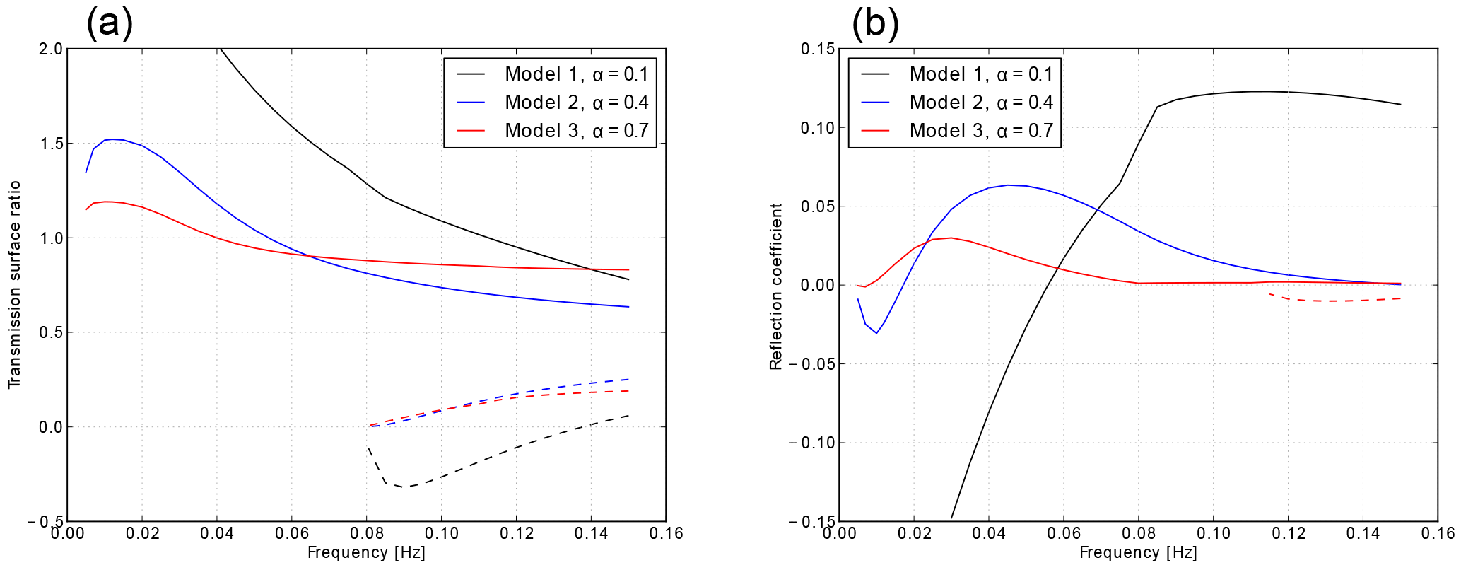
Figure B3 Love wave surface transmission ratios (a) and reflection coefficients (b) for an incident fundamental mode propagating in the forward direction through three varieties of Alsop66's M-discontinuity step model. The model varieties are indicated by the geometrical parameter α (see Fig. 13 of Alsop66 for its definition). Values obtained with SWRT (solid lines for the fundamental mode, dashed lines for the first overtone) are nearly identical to the original results of Alsop66 (its Figs. 14 and 15). The only apparent discrepancy is in the sign of the transmitted first higher mode for the α=0.1 model, which was wrongly plotted by Alsop66.