Apsu: a wireless multichannel receiver system for surface nuclear magnetic resonance groundwater investigations

Surface nuclear magnetic resonance (surface NMR) has the potential to be an important geophysical method for groundwater investigations, but the technique suffers from a poor signal-to-noise ratio (SNR) and long measurement times. We present a new wireless, multichannel surface-NMR receiver system (called Apsu) designed to improve field deployability and minimize instrument dead time. It is a distributed wireless system consisting of a central unit and independently operated data acquisition boxes each with three channels that measure either the NMR signal or noise for reference noise cancellation. Communication between the central unit and the data acquisition boxes is done through long-distance Wi-Fi and recordings are retrieved in real time. The receiver system employs differential coils with low-noise preamplifiers and high-resolution wide dynamic-range acquisition boards. Each channel contains multistage amplifiers, short settling-time filters, and two 24 bit analog-to-digital converters in dual-gain mode sampling at 31.25 kHz. The system timing is controlled by GPS clock, and sample jitter between channels is less than 12 ns. Separated transmitter/receiver coils and continuous acquisition allow NMR signals to be measured with zero instrument dead time. In processed data, analog and digital filters cause an effective dead time of 5.8 ms including excitation current decay. Synchronization with an independently operated transmitter system is done with a current probe monitoring the NMR excitation pulses. The noise density measured in a shorted-input test is 1.8 nV Hz${}^{-\mathrm{1}/\mathrm{2}}$. We verify the accuracy of the receiver system with measurements of a magnetic dipole source and by comparing our NMR data with data obtained using an existing commercial instrument. The applicability of the system for reference noise cancellation is validated with field data.

1 Introduction

Sustainable groundwater extraction is critical to ensure continuous access to drinking water and irrigation water in countries all over the world. Geophysical methods can supply spatially dense and cost-effective hydrogeological information to guide groundwater extraction (Auken et al., 2003; Yaramanci et al., 2002). Surface nuclear magnetic resonance (surface NMR) is one such method featuring a direct sensitivity to aquifer properties such as water content and pore geometry (Behroozmand et al., 2015; Knight et al., 2012; Legchenko et al., 2002). By stimulating the unbalanced spins of hydrogen in groundwater with an excitation pulse (generated using a surface wire-loop transmitter) in the background of the static Earth's magnetic field, the surface-NMR receiver can record a free induction decay (FID) signal released as the spins realign with the static magnetic field. The signal amplitude is proportional to the water content of the investigated sample volume and to the square of the static magnetic field B₀ (Hertrich, 2008; Legchenko and Valla, 2002; Weichman et al., 2000). The signal frequency, known as the Larmor frequency f_L, is determined by the proton gyromagnetic ratio and B₀. The Earth's magnetic field ranges from 25 to 65 µT, resulting in signal amplitudes on the order of nanovolts and Larmor frequencies ranging from 1 to 2.8 kHz. These small measured signals can easily be swamped by external noise sources, including power line harmonics, spherics, electric fence spikes, and other anthropogenic installations (Costabel and Müller-Petke, 2014; Larsen et al., 2014). Besides these noise sources, the inherent noise in the receiver can also dominate the NMR signal. The low signal-to-noise ratio (SNR) of measurements presents a major obstacle to the application of surface NMR.

The first surface-NMR instruments used a single coil for both excitation and signal measurement (Legchenko and Valla, 2002; Semenov, 1987). Later instruments introduced dedicated reference coils for simultaneous noise measurements used for reference noise cancellation to improve the SNR (Radic, 2006; Walsh, 2008). State-of-the-art multichannel surface-NMR instruments are centralized systems, where the signal coil and reference coils are wired to a central controller. Although these systems have significantly advanced surface NMR, the current methodology also has a number of shortcomings. First, requiring a physical link (i.e., a wire) between the reference coil and the central controller limits the maximum separation between the signal coil and reference coils. If the reference coil is placed too close to the signal coil, it may unintentionally detect the NMR signal, which would lead to the cancellation of the NMR signal in the processed data (Larsen and Behroozmand, 2016). Second, the link cables are laborious to lay out in the field and increase setup and teardown times, especially in scenarios where a large number of coils are used, as in surface-NMR tomography (Jiang et al., 2014; Legchenko et al., 2011). Third, a hardware-related instrument dead time is introduced when the same coil is used for transmitting the excitation pulse and receiving the NMR signal. We define the instrument dead time to be the portion of the signal that cannot be measured because of switching electromechanical relays. The instrument dead time prevents measurement of the initial high-amplitude part of the FID signals and reduces the SNR (Dlugosch et al., 2011; Walsh et al., 2011). These shortcomings can be addressed by employing a different surface-NMR instrumentation where one transmitter (Tx) coil is used to emit the excitation pulse and small dedicated receiver (Rx) coils, wirelessly connected to a central unit, continuously record the NMR signal and reference noise.

Wirelessly operated coils eliminate the need for cables to physically link the Rx coils to the central controller and grant increased flexibility. This is beneficial for field work; for example, if several soundings are being performed in the same survey area, the same placement of the reference coils can be employed and only the transmitter and signal coil must be moved between soundings. In two- and three-dimensional groundwater investigations, a receiver system with an array of wirelessly connected signal receiving coils distributed throughout the study area has great potential to provide significant reductions in field measurement times.

We present a new multichannel surface-NMR receiver system, called Apsu, consisting of a central unit (ApsuMaster) with wireless connections to data acquisition boxes (ApsuRx). Each ApsuRx unit can be connected with up to three Rx coils measuring signal or noise. The Rx coils are directly attached to preamplifiers, and short cables pass the amplified signals to the ApsuRx units where the signals are further processed using multistage amplifiers, and bandpass filters and are sampled by two 24 bit analog-to-digital converters (ADCs) in dual-gain mode. Accurate timing is obtained by synchronizing the ApsuRx with the GPS clock. Communication and data transfer between the ApsuMaster and ApsuRx are done via long-distance Wi-Fi. The performance of the receiver system is validated with laboratory and field measurements, in particular a comparison with a GMR (Vista Clara Inc., USA) system gives practically equivalent NMR signals.

2 Receiver design

The field setup of our wireless multichannel surface-NMR receiver system Apsu operating independently of a transmitter is shown in Fig. 1. One signal channel is dedicated to synchronizing the receiver system to an independently operating transmitter system by detecting the turn-on time and waveform of NMR excitation pulses using a current probe mounted on the transmitter cable. One or more Rx coils are placed inside the Tx coil and connected to the signal channels for measuring the NMR signal. Additional noise Rx coils and reference channels are placed distant to the Tx coil for continuous recording of noise. The channels used for signal detection and for noise recording are identical and they are configured remotely by the ApsuMaster, for instance, the gain factors and synchronization time. The ApsuMaster is a compact industrial PC running the instrument software and is connected to an array of Wi-Fi antennas. All channels are time-synchronized using GPS and are linked to the ApsuMaster through a Wi-Fi network. The ApsuMaster retrieves the measured time series from all channels in real time for processing and display. In the case of a lost Wi-Fi connection, data can be retrieved asynchronously in the field or be accessed with an FTP client after the measurement.

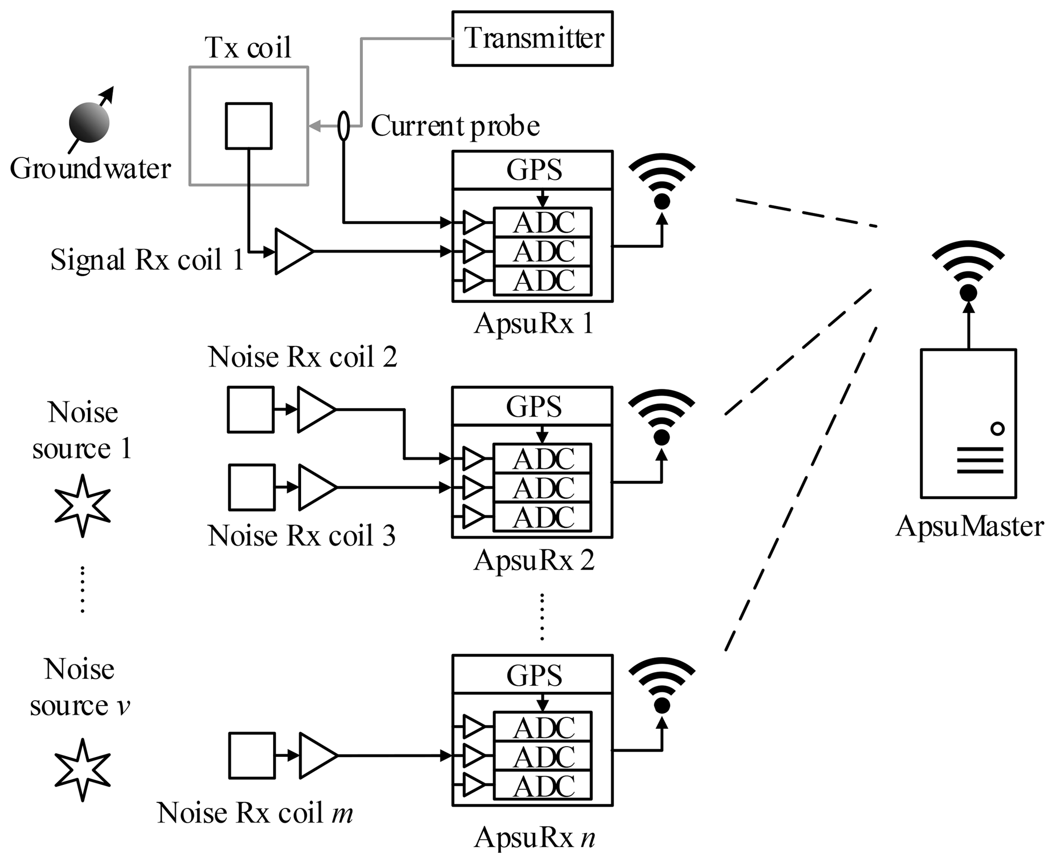
Figure 1 Setup of the wireless multichannel surface-NMR receiver Apsu. Each ApsuRx contains three GPS-synchronized channels. A current probe is connected to a channel of ApsuRx1 detecting the pulse, and signal Rx coil 1 is connected to the other channels recording the NMR signal. In the vicinity of noise sources, ApsuRx2–ApsuRxn and noise Rx coil 2–m are deployed.

2.1 Rx coil with a preamplifier

The voltage induced in an Rx coil is proportional to the area-turn product, and the signal amplitude derived from it should be significantly higher than the receiver-inherent noise. Surface-NMR signals are inherently weak but they can be magnified by high-quality factor Rx coils tuned with external capacitors. However, tuned Rx coils have long transient response times, which contributes to a long filter settling time and gives rise to near-exponential decaying oscillations in the frequency band of NMR signals if impulsive excitations (i.e., lighting and electric fence discharge) are present. Moreover, the quality factors must be calibrated before measurements. The GMR and MRS-MIDI employ the untuned coil (Radic, 2006; Walsh, 2008); however, the construction of these coils is quite different from the construction used in Apsu. To reduce filter settling time and calibration procedures, untuned Rx coils are used in our instrument.

In standard surface-NMR measurements, the area-turn product of Rx coils ranges from 1000 to 10 000 m². Larger Rx coils gives higher signal amplitude, but they take more time and manpower to deploy in surveys. Another drawback is that larger Rx coils have high inductance and parasitic capacitance, resulting in a lower cutoff frequency and significant phase shift of the surface-NMR signal. In addition, SNR remains unimproved for larger coils, once the area-turn product is high enough. In this limit, the inherent noise in the receiver electronics is negligible compared to the signal and noise coupled inductively into the coil. Increasing the area-turn product gives a corresponding increase in both signal and coupled noise and SNR is unimproved.

Based on noise measurements conducted at different sites in Denmark, a typical value for the stochastic background noise density is 0.02 nV m⁻² Hz${}^{-\mathrm{1}/\mathrm{2}}$) (Nyboe and Sørensen, 2012). Considering an area-turn product of 1000 m², the external noise will be about 10 times stronger than our receiver-inherent noise, as discussed later. The Rx coils used for the measurements presented here are 10 m × 10 m eight-turn differential coils (Fig. 2), with resistance R=17.4 Ω, self-inductance L=1.85 mH, and parasitic capacitance C=7.4 nF. A differential Rx coil is beneficial to cancel the common-mode noise, and it is able to reduce the Johnson noise of the coil by half (Chen et al., 2015; Nyboe and Sørensen, 2012). The typical common-mode noise is the induced noise in the leading cable and the wiring of the acquisition board by the coupling noise. The cutoff frequency of these Rx coils is 43 kHz, which is approximately 20 times higher than the local Larmor frequency; hence, the amplitude and phase distortion of the NMR signal are negligible.

Damping resistors R_d are used to set the Rx coil into the critically damped state or slightly overdamped. The damping resistance is given by Lehtonen and Hällström (2017),

$$\begin{array}{}\text{(1)}& {\displaystyle }{R}_{\mathrm{d}}\ge {\displaystyle \frac{L}{RC+\mathrm{2}\sqrt{LC}}}.\end{array}$$

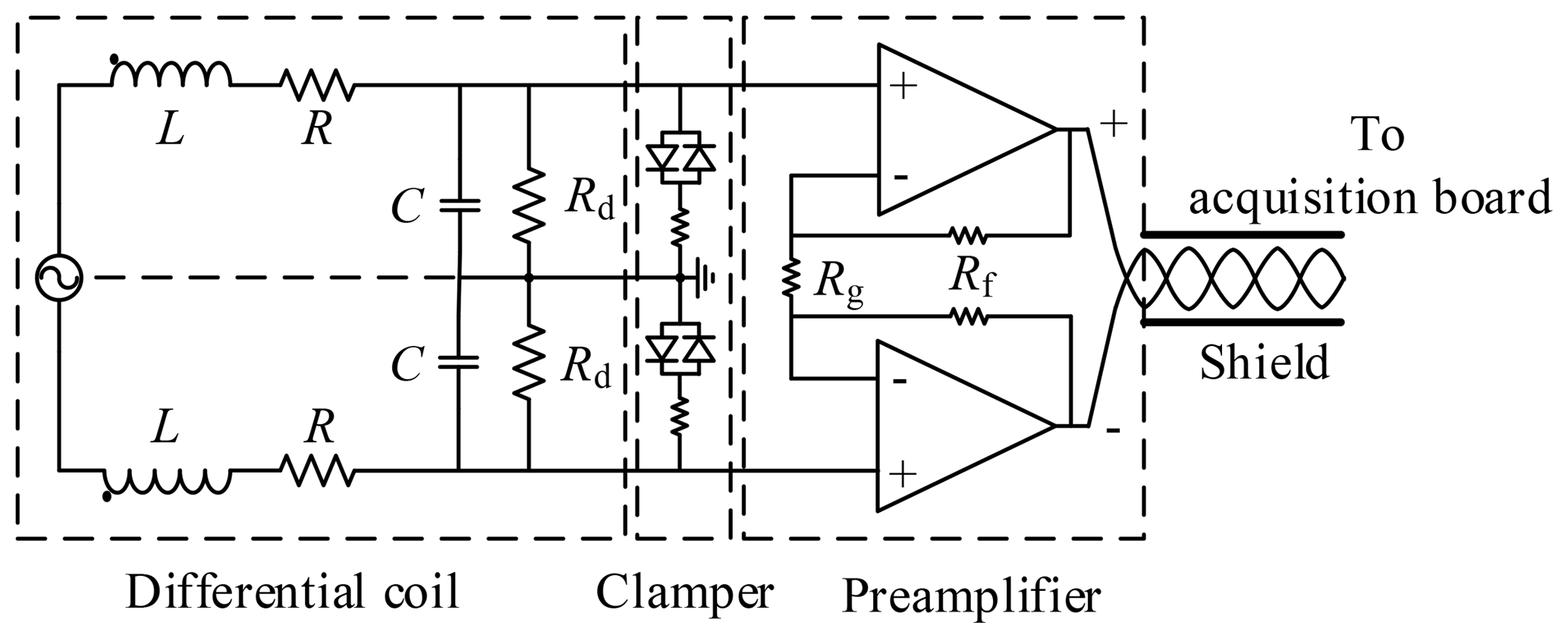
Figure 2 Schematic diagram of the differential Rx coil and preamplifier. A diode clamper is used to protect the amplifiers from overvoltage during strong Tx pulses.

A preamplifier is mounted directly at the coil to amplify the signal before transmission. The preamplifier is a very low-noise, low-distortion operational amplifier with a typical input noise voltage of 0.9 nV Hz${}^{-\mathrm{1}/\mathrm{2}}$ in the 1–3 kHz range. The amplifier gain is 21, determined by gain resistor R_g and feedback resistor R_f. The low-resistance resistors used in the preamplifier reduce the internal noise in the preamplifier.

The Rx coil and preamplifier are physically connected during the entire measurement, so the induced voltage can exceed the maximum input range of the preamplifier during the surface-NMR excitation pulse. To protect against overvoltage, a clamper consisting of two diodes in inverse parallel is used to clip the voltage to a safe range if the amplitude exceeds the forward voltage of the diode. The output signal from the preamplifier is sent to the acquisition board through a 5 m long twisted and shielded cable.

The amplifiers used in the acquisition board have the same noise levels as the preamplifier, so the receiver-inherent input noise density, n_i, is determined by the preamplifier noise. The noise density in the preamplifier is composed of thermal, voltage e_n, and current noise i_n:

$$\begin{array}{}\text{(2)}& {\displaystyle }{n}_i=\sqrt{\mathrm{2}[\mathrm{4}kT\left(R_{\mathrm{s}}+R_{\mathrm{a}}\right)+e_{\mathrm{n}}^{\mathrm{2}}+{\left(i_{\mathrm{n}}{R}_{\mathrm{a}}\right)}^{\mathrm{2}}+(i_{\mathrm{n}}Z{)}^{\mathrm{2}}]},\end{array}$$

where k is the Boltzmann constant and T is the temperature and

$$\begin{array}{ll}{\displaystyle }& {\displaystyle }{R}_{\mathrm{s}}={\displaystyle \frac{R{R}_{\mathrm{d}}}{R+R_{\mathrm{d}}}},R_{\mathrm{a}}={\displaystyle \frac{R_{\mathrm{f}}{R}_{\mathrm{g}}/\mathrm{2}}{R_{\mathrm{f}}+R_{\mathrm{g}}/\mathrm{2}}},\\ {\displaystyle }& {\displaystyle }Z={\displaystyle \frac{R_{\mathrm{d}}(j\mathit{\omega }L+R)}{(j\mathit{\omega }L+R)(j\mathit{\omega }{R}_{\mathrm{d}}C+\mathrm{1})+R_{\mathrm{d}}}},\end{array}$$

where ω is the angular frequency. The theoretical inherent-noise density is 1.8 nV Hz${}^{-\mathrm{1}/\mathrm{2}}$ at 2 kHz. In measurements, an N-fold stacking reduces the inherent noise by a factor of $\sqrt{N}$.

2.2 Acquisition board

The acquisition board is a custom made board containing a low-power consumption field-programmable gate array (FPGA) and three high-resolution channels with multistage amplifiers, filters, and 24 bit ADCs. A block diagram of the acquisition board is shown in Fig. 3.

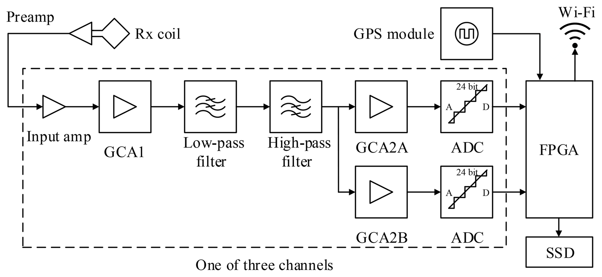
Figure 3 Block diagram of acquisition board. Note that each ApsuRx contains three duplicated channels, and only one of them is illustrated in the dashed box.

The analog circuit of the acquisition board employs differential signaling in accordance with the Rx coil design to cancel common-mode noise. The input amplifier is low-noise, with a fixed gain of 21. There are two stages of gain-controlled amplifiers (GCAs) and their gain factors are remotely adjusted by the ApsuMaster according to the local noise level.

Although the Rx coils attenuate the noise with a frequency higher than the cutoff frequency, the signals input to the ApsuRx are normally severely affected by externally coupled noise. Saturation of the second-stage GCA due to externally coupled noise is avoided by applying filter that remove out-of-band noise before the signal reaches this amplifier. The transient response of the bandpass filters contributes to the filter settling time. The transient response rate of a second-order filter is characterized by the settling time t_s (Angeles, 2011):

$$\begin{array}{}\text{(3)}& t_{\mathrm{s}}={\displaystyle \frac{\mathrm{4}}{\mathit{\zeta }{\mathit{\omega }}_{\mathrm{c}}}},\end{array}$$

where ζ is the damping ratio and ω_c is the cutoff frequency. We utilize a second-order low-pass filter and a second-order high-pass filter in cascade for noise reduction. The low-pass filter with a cutoff frequency of 5 kHz reduces radio frequency noise, and the high-pass filter with a cutoff frequency of 1 kHz is responsible for reducing low-order power line harmonics. The filters have an overall settling time of only 0.42 ms preserving the early-time signal. The phase shift imposed on the NMR signal by the filters is determined by f_L and can be modeled and calibrated.

The second GCA operates in dual-gain mode, and the two signals are independently quantized by two 24 bit ADCs. The high-accuracy ADC has a typical SNR of 113.5 dB. In normal cases, the signal from the high-gain path is used to maintain a high resolution. In segments of data where strong noise, e.g., from spikes, saturates the high-gain path, the signal in the low-gain path can be substituted and unusable segments of data are avoided. To replace the saturated data in the high-gain path, all the samples are converted to the true input voltage after being divided by the gain factor. The dynamic range is increased by the gain factor ratio between the high-gain path and low-gain path.

To minimize the inherent noise of ApsuRx and obtain the optimal resolution, the overall gain factor through the measurement channel must be chosen so that the ADC quantization noise is much smaller than the noise from the analog circuit. The ADC quantization noise density, n_ADC, depends on the SNR of the ADC, SNR_ADC, and the sampling frequency f_s (Walden, 1999):

$$\begin{array}{}\text{(4)}& {\displaystyle }{n}_{\mathrm{ADC}}={\displaystyle \frac{V_{\mathrm{FS}}}{{\mathrm{10}}^{{\text{SNR}}_{\mathrm{ADC}}/\mathrm{20}}}}{\displaystyle \frac{\mathrm{1}}{\sqrt{f_{\mathrm{s}}/\mathrm{2}}}},\end{array}$$

where V_FS is the 5 V full-scale voltage of the ADC. For a sampling frequency of 31.25 kHz, the ADC quantization noise density is 84.5 nV Hz${}^{-\mathrm{1}/\mathrm{2}}$. Considering the 1.8 nV Hz${}^{-\mathrm{1}/\mathrm{2}}$ analog circuit noise density, the overall gain factor must be at least 500 for a 10 : 1 ratio. The minimum and maximum gain factors of the ApsuRx amplifier chain are 441 and 194 481, respectively.

The FPGA has a dual-core ARM (advanced RISC machine) processing system (PS) part and a programmable logic (PL) part in a single device. The acquisition board contains two input–output (I/O) headers that connect to I/O banks on the PL side and is used as an embedded system on module. To fulfill the critical timing requirements in signal acquisition, blocks for synchronizing the wirelessly connected ApsuRx units and reading the ADCs are implemented in the PL part. The synchronization block is based on a D flip–flop triggered by the rising edge of the GPS pulse and is remotely controlled by the ApsuMaster. The ADC reading block for each channel uses the serial peripheral interface (SPI) bus to read out the two ADCs in daisy chain, which ensures the high-gain path and low-gain path are sampled simultaneously. Another block receives and decodes the time and location information from the GPS module. The GPS time is refreshed every second and used as the reference for timing synchronization between ApsuRx units.

The two ARM processors in the PS are programmed in asymmetric multiprocessing (AMP) mode: one is running an embedded Linux system and the other executes the bare-metal applications. The AMP mode takes advantage of the efficiency of a bare-metal machine in real-time applications and the flexibility of the Linux system in networking and massive data operating programming. The peripherals of the PS include 1 GB of memory, a gigabit Ethernet, a micro SD, and a USB port. The gigabit Ethernet is connected to a Wi-Fi antenna, and the USB port is connected to a 128 GB solid-state drive (SSD) for data logging. The Linux system is responsible for communicating with the ApsuMaster through Wi-Fi and storing and retrieving data, as well as controlling the bare-metal processor. The bare-metal processor is interrupt-driven and reads samples from the ADC reading block in the PL part and writes them into the shared memory. Subsequently, the data are grabbed and stored on the SSD by the Linux system. When the ApsuMaster requests data from the ApsuRx, the Linux system reads the data from the SSD and transfers it to the ApsuMaster through Wi-Fi. ApsuRx also contains an FTP server, and the collected data can be accessed through an FTP client software after the measurement. The acquisition board, GPS antenna, and a rechargeable 9 Ah lithium battery are assembled in a waterproof case (Fig. 4).

Figure 4 (a) ApsuRx. The breakout box of ApsuRx provides plugs for three signal inputs, power, and Wi-Fi antenna connection. The GPS antenna in the top-right corner is used for time synchronization. (b) ApsuMaster is connected to the Wi-Fi tower which consists of a array of Wi-Fi antennas working in the access point mode.

2.3 Synchronization between channels

The timing accuracy and stability of the receiver system are of fundamental importance for obtaining high-quality data. Any significant timing jitter or uneven sampling frequencies between channels will significantly reduce the efficiency of the reference noise cancellation and phase determination of the NMR signal. Therefore, the system is designed with strict requirements for timing. We utilize a GPS timing module to maintain high timing accuracy. The GPS synchronization technique is widely applied in the seismic system (Sens-Schönfelder, 2008). The GPS module provides two outputs: a pulse per second (PPS) signal and a reference clock. The PPS pulse with a jitter jt_pps less than 11 ns is used to trigger the sample-start clock of the ADCs. Triggering the sample-start clocks between the ApsuRx units is achieved with the following procedures: (1) the ApsuMaster sends a command to the ApsuRx units indicating the scheduled synchronization time; (2) all the ApsuRx units enable the synchronization blocks; (3) reset pulses for all the ADCs are generated at the rising edge of the scheduled PPS; and (4) the channels output valid data after a fixed settling time of the ADC's digital filters, which is 2370 cycles of the driving clock. Following these procedures, all ApsuRx units collect data continuously until the next synchronization action.

To ensure that all ApsuRx units use the identical sampling frequency, the ADCs are driven by a low-jitter 1 MHz GPS-derived reference clock. The mean error μ(Δf_clk) and standard deviation σ(Δf_clk) of the reference clock are $\mathrm{6.2}\times {\mathrm{10}}^{-\mathrm{5}}$ and $\mathrm{7.0}\times {\mathrm{10}}^{-\mathrm{4}}$ Hz, respectively. The frequency of the reference clock and the decimation ratio of the ADC λ=32 result in a sampling rate f_s of 31.25 kHz.

The jitter of the PPS, the instability of the reference clock, and the lack of synchronization with the 200 MHz main clock f_mclk of the FPGA all contribute to the sample-start jitter jt_sync between channels, which is calculated as

$$\begin{array}{}\text{(5)}& {\displaystyle }{\text{jt}}_{\mathrm{sync}}=\sqrt{{\text{jt}}_{\mathrm{pps}}^{\mathrm{2}}+(\mathrm{2370}\times {\displaystyle \frac{\mathit{\sigma }\left(\mathrm{\Delta }{f}_{\mathrm{clk}}\right)}{f_{\mathrm{clk}}^{\mathrm{2}}}}{)}^{\mathrm{2}}+({\displaystyle \frac{\mathrm{1}}{f_{\mathrm{mclk}}}}{)}^{\mathrm{2}}}.\end{array}$$

The GPS module only needs the signal from a single satellite to provide accurate pulse timing, and it works nicely in practice, even with limited field of view and cloud cover. Compared with the PPS jitter, the frequency error of f_clk contributes very little to the synchronization jitter. The synchronization jitter jt_sync is less than 12 ns, which is much smaller than the 32 µs sample period.

Once the mth ADC is synchronized at time t_sync(m), every new sample will be labeled with a unique time stamp t_ID(m,n). The recordings are stored in a data structure in the SSD. Each structure consists of a 1 s time series and the corresponding data header. The data header indicates the properties of the time series, such as gain factors, t_sync(m), and t_ID(m,n). To align the samples from different channels after they are transferred to the ApsuMaster, the global time t_g(m,n) should be equal for each sample:

$$\begin{array}{}\text{(6)}& {\displaystyle }{t}_{\mathrm{g}}(m,n)=t_{\mathrm{sync}}\left(m\right)+{\displaystyle \frac{t_{\mathrm{ID}}(m,n)}{f_{\mathrm{s}}}}.\end{array}$$

Due to the frequency error of the ADC clock in the different channels, there is a time shift t_shift between the two aligned samples after the channels have been synchronized for T_N seconds. The time shift between samples is written as

$$\begin{array}{}\text{(7)}& t_{\mathrm{shift}}={\text{jt}}_{\mathrm{sync}}+\mathit{\lambda }{T}_N{f}_{\mathrm{s}}{\displaystyle \frac{\mathit{\mu }\left(\mathrm{\Delta }{f}_{\mathrm{clk}}\right)}{f_{\mathrm{clk}}^{\mathrm{2}}}}.\end{array}$$

A time shift of less than 0.22 µs is generated per hour in our multichannel receiver system. Hence, the time shift in one measurement can be ignored compared to the cycle of the NMR signal.

3 Wireless communication network

A design goal of the system is to be able to conduct surface-NMR measurements with wireless communication to remote coils located up to 1 km away. Besides coverage, link speed is another crucial requirement of the network. A 1 s time series sampled in 24 bits at 31.25 kHz plus data header amounts to 96 kB, and as each ApsuRx unit contains three channels, the transfer speed should be higher than 288 kB s⁻¹ for real-time operation. We used an outdoor long-distance Wi-Fi, which has a dual-polarized directional antenna and a high transmission power. This Wi-Fi antenna provides a link speed of up to 300 Mbps and a maximum coverage range of 10 km along the direction of orientation.

3.1 Wi-Fi network

The wireless network consists of the ApsuMaster and a number of ApsuRx units (Fig. 5). The ApsuMaster is based on a high-performance, compact industrial PC installed in a solid, waterproof case (Fig. 4). A Wi-Fi tower consisting of an array of Wi-Fi antennas working in access point (AP) mode is connected to the ApsuMaster. The measurements retrieved by the ApsuMaster can be monitored through a wireless remote desktop connection (RDC). The ApsuRx units are each attached to a single Wi-Fi antenna set to client mode.

Figure 5 Topology of the network of wireless surface-NMR instrument Apsu. The network mask is 255.255.255.0, and only the host numbers of the IP address are shown.

The signal beam width of each Wi-Fi antenna is 45^∘ in the horizontal plane and 30^∘ in the vertical plane. To achieve full 360^∘ coverage, eight Wi-Fi antennas are used in the Wi-Fi tower. The antennas are mounted at the top of an adjustable tripod and encapsulated in a waterproof container (Fig. 4). Each antenna forwards power and a digital link to the next Wi-Fi antenna in the Wi-Fi tower. By daisy-chaining the eight Wi-Fi antennas, the Wi-Fi tower can be connected to the ApsuMaster through a single Cat5e cable. The eight Wi-Fi antennas connected to the ApsuMaster not only provide better coverage but also improve the overall network-capacity and transfer speed. The client Wi-Fi antennas in the ApsuRx automatically connect to the AP in the Wi-Fi tower which provides the strongest radio signal for it. To obtain a stable wireless link, the horizontal and vertical angles of the Wi-Fi antennas in the ApsuRx are adjusted to face the Wi-Fi tower. The power consumption of an ApsuRx including the Wi-Fi antenna is around 12 W, and 6–8 h of data collection can be performed on a single charge of a 9 Ah battery. Batteries can be hot-swapped in the system without interrupting data collection.

3.2 Communication protocol

Communication between the ApsuMaster and ApsuRx in the receiver system is done using stream sockets on top of a transmission control protocol/internet protocol (TCP/IP). A server–client pair is established between the ApsuMaster and each ApsuRx. Each server–client pair runs in its own thread to keep communication with each ApsuRx unit independent. At start-up, each server socket in the ApsuMaster listens for a connection request from the corresponding ApsuRx. Once the connection is established, the client socket can send commands to the ApsuRx. In the ApsuRx, the server socket receives commands from the ApsuMaster, and the client socket responds to it by sending a data package to the ApsuMaster server socket. The communication between the ApsuMaster and each ApsuRx is a full-duplex transmission pipe. Software in the ApsuMaster handles the TCP/IP communication and processes the retrieved data.

A custom communication frame protocol is defined for the decoding of different commands from the ApsuMaster. The command frame sent from the ApsuMaster to the ApsuRx is a binary sequence including start code, frame length, command ID, and command parameters. By defining different command IDs both in the ApsuMaster and the ApsuRx, each ApsuRx can perform independent actions such as gain factor setting, channel synchronization, status retrieval, and data transfer.

4 Performance verification

4.1 Shorted-input noise test

We verified the inherent noise properties of the receiver system by shorting the input to each preamplifier on two measurement channels and recording noise simultaneously from the two channels. After the subtraction of DC offsets, the samples recorded in 1 s are shown in Fig. 6a.

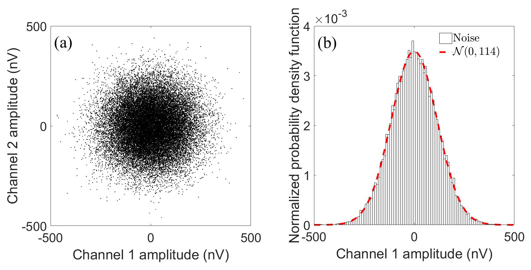
Figure 6 (a) Scatterplot of 1 s of samples from two channels recorded with shorted inputs on the preamplifiers; DC offsets are removed. (b) Normalized PDF histogram of channel 1 noise amplitudes. The width of the bins is 10 nV, and there are 100 bins in total. The red dashed line is the PDF curve of the Gaussian distribution with zero mean and a standard deviation of 114 nV.

The voltages are in the range of ±500 nV, and the root mean square (rms) values n_rms for the two channels are both 114 nV. We found no correlation between measurements from the two channels, and the histogram distribution of voltages matches the probability density function (PDF) of Gaussian noise (Fig. 6b), implying that the measured voltages are receiver-inherent noise. The inherent noise density of the ApsuRx can be calculated as

$$\begin{array}{}\text{(8)}& {\displaystyle }{n}_{\mathrm{d}}={\displaystyle \frac{n_{\mathrm{rms}}}{\sqrt{f_{\mathrm{high}}-f_{\mathrm{low}}}}},\end{array}$$

where f_low and f_high are the cutoff frequencies of the bandpass filter in ApsuRx. The noise spectral density in a 1 s measurement is 1.8±0.3 nV Hz${}^{-\mathrm{1}/\mathrm{2}}$ in the passband at 2 kHz. This measurement is in good agreement with the theoretical noise density of 1.8 nV Hz${}^{-\mathrm{1}/\mathrm{2}}$ in Sect. 2.1.

4.2 Measurement accuracy

The accuracy of the receiver system was validated with measurements of a magnetic dipole source. The magnetic dipole was a one-turn, 5 m × 5 m square coil driven by a signal generator and an audio amplifier. The Rx coil was a 16-turn, 5 m × 5 m square coil. The center-to-center distance between the two coils was 50 m. The distance between the two coils was 10 times the side length, and the transmitter magnetic field can therefore be approximated as a magnetic dipole. The theoretical receiver signal caused by the current in a coplanar transmitter coil is given as

$$\begin{array}{}\text{(9)}& {\displaystyle }V\left(t\right)={\displaystyle \frac{{\mathit{\mu }}_{\mathrm{0}}\mathit{\omega }I\left(t\right)A_{\mathrm{t}}{A}_{\mathrm{r}}}{\mathrm{4}\mathit{\pi }{r}^{\mathrm{3}}}},\end{array}$$

where μ₀ denotes magnetic permeability in the air, r is the distance between the coils, and A_t and A_r are the area-turn products of the two coils. The signal generator output was a 2125 Hz sinusoid, and the transmitter current was adjusted from 0.1 to 5 A. The current I(t) was determined by a commercial current probe attached to an oscilloscope. The receiver signal amplitudes were obtained by a Fourier transform of the measured time series. The receiver signal amplitude is plotted against the transmitter current along with the theoretical prediction in Fig. 7.

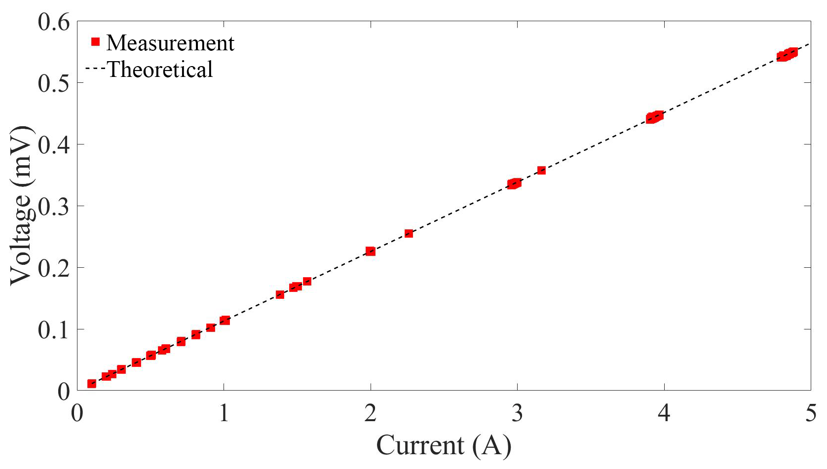
Figure 7 Comparison between measured (red squares) and theoretical (black line) signal amplitudes from a magnetic dipole source.

We observed that the received signal amplitude increased linearly with the transmitter current, and all measurements match the theoretical values with a less than 1 % relative error, confirming the accuracy of the receiver system.

4.3 Reference noise cancellation

We tested the applicability of the reference noise cancellation (RNC) scheme with wirelessly connected receiver coils using a synthetic surface-NMR signal embedded in noise-only records. The synthetic signal was chosen as this makes it possible to compare the output of the processed data with the expected result. Noise-only data were collected near Silkeborg, Denmark. One ApsuRx served as the “signal” receiver and was connected to an Rx coil. A second ApsuRx, located approximately 200 m away in the east, served as the remote reference receiver and was connected to two Rx coils located to the north and south of the reference receiver. The distance between the two reference coils was approximately 100 m. All coils were 5 m × 5 m 16-turn coils

The data from the three coils were dominated by power line harmonics and stochastic background noise. A mono-exponential synthetic NMR signal with parameters E₀=100 nV, $T_{\mathrm{2}}^{*}=\mathrm{200}$ ms, and f_L=2124 Hz was embedded in the signal data. The surface-NMR data were processed using the scheme described by Müller-Petke et al. (2016). The data were bandpass filtered with a 500 Hz bandwidth filter centered at the Larmor frequency. Power line harmonics were subtracted from all data sets using the model-based method (Larsen et al., 2014). The rms value of noise in the original data was 3320 nV. The rms value decreased to 147 nV after bandpass filtering and to 85 nV after harmonic subtraction. Reference noise cancellation reduced the rms value to 67 nV using noise from one reference coil and to 62 nV with noise from two reference coils. Both the data before and after RNC are used to extract envelopes through digital quadrature detection and stacking. Figure 8 shows the two envelopes after quadratic detection and 18 times stacking; the blue solid line and black dashed line are the results processed without and with RNC. The rms values of noise with and without RNC after stacking are 18 and 30 nV, respectively.

Compared with the envelope without RNC, the result processed with RNC matches better with the synthetic envelope (red dotted line). The SNR for the two envelopes is 0.4 and 5.1 dB, respectively, which implies an SNR improvement of 4.7 dB with RNC. The SNR of an envelope is defined as

$$\begin{array}{}\text{(10)}& {\displaystyle }\text{SNR}=\mathrm{10}\log \left({\displaystyle \frac{{\sum }_{k=\mathrm{0}}^N{\left(E_{\mathrm{0}}{e}^{-t\left(k\right)/T_{\mathrm{2}}^{*}}\right)}^{\mathrm{2}}}{{\sum }_{k=\mathrm{0}}^N{\left(E\left(k\right)-E_{\mathrm{0}}{e}^{-t\left(k\right)/T_{\mathrm{2}}^{*}}\right)}^{\mathrm{2}}}}\right),\end{array}$$

where E is the envelope obtained with noise, $s_{\mathrm{0}}{e}^{-t\left(k\right)/T_{\mathrm{2}}^{*}}$ is the synthetic signal and N is the datum of envelope. Following all processing steps, a mono-exponential model was fitted to the envelope of the data. With RNC, the fitted parameters are $E_{\mathrm{0}}=\mathrm{102}\pm \mathrm{6}$ nV and $T_{\mathrm{2}}^{*}=\mathrm{193}\pm \mathrm{11}$ ms which are close to the parameters of the synthetic NMR signal. If the RNC step is excluded, the envelope is noisier and the fitted parameters are $E_{\mathrm{0}}=\mathrm{132}\pm \mathrm{16}$ nV and $T_{\mathrm{2}}^{*}=\mathrm{150}\pm \mathrm{23}$ ms. These results show that RNC can be performed with the new instrument and improves SNR and the accuracy of the estimated parameters.

Figure 8 Envelopes extracted with and without RNC technique to demonstrate the SNR improvements of RNC. The red dotted line is the synthetic envelope. The blue solid line and black dashed line are the results processed without and with RNC.

5 Field measurement

5.1 Field validations

To validate the reliability of the receiver system for groundwater investigations, a field measurement was conducted at the Schillerslage test site near Hanover, Germany. The geological properties of the site have been characterized in previous studies (Grombacher et al., 2016; Müller-Petke et al., 2011). Lithological logging shows that the test site is characterized by two sandy aquifer layers. The water table is typically 1.5–3 m below the surface and partially fills the upper aquifer consisting of medium to coarse sands with inter-bedded peat layers down to about 11 m. A glacial till with fine sands separating the upper aquifer from the lower is about 6 m thick. The lower aquifer consisting of medium sands is about 3 m thick, and bedrock is found beneath these layers.

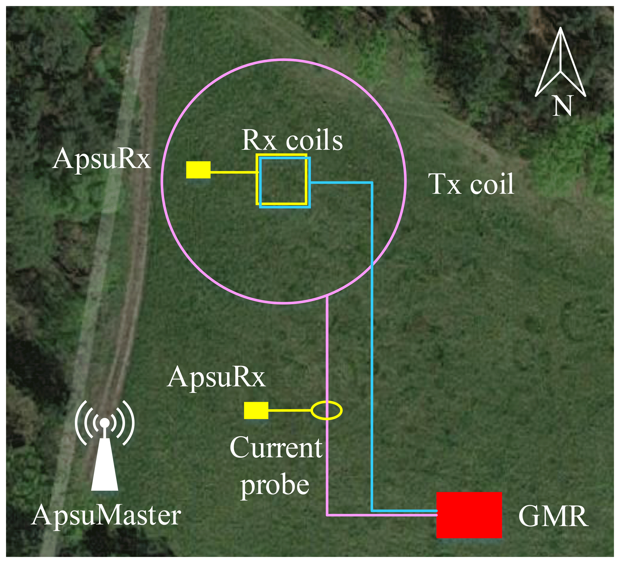
Figure 9 Field measurement setup with Apsu and GMR at the Schillerslage test site near Hanover, Germany.

The field setup is illustrated in Fig. 9. A commercial surface-NMR instrument, the GMR, Vista Clara, was used for comparison. The GMR had a dual purpose as it is a well-established surface-NMR Rx system to compare with and it also supplied the transmission pulses needed for our receiver system. The GMR excitation pulses were transmitted using a 60 m diameter circular Tx coil (light purple circle), and the NMR signals were recorded with a 10 m × 10 m, 12-turn square Rx coil (light blue square, area-turn product 1200 m²) located at the center of the Tx coil. The Apsu receiver system consists of one Apsu Master and two ApsuRx; one channel in an ApsuRx was connected to a 10 m × 10 m, eight-turn square Rx coil (yellow square, area-turn product 800 m²) overlapped with the GMR Rx coil. One channel of another ApsuRx unit was connected to a high-bandwidth current probe (yellow ellipse) to detect the turn-on time of the GMR transmitter. The ApsuMaster shown in the lower left of Fig. 9 controlled the data acquisition and retrieval in the ApsuRx units through wireless communication. The Larmor frequency at the site was 2104 Hz. In the measurements, 22 pulse moments sampling the interval from 0.09 to 10 As were used, all with a 40 ms pulse duration. Each pulse moment was repeated 28 times for stacking.

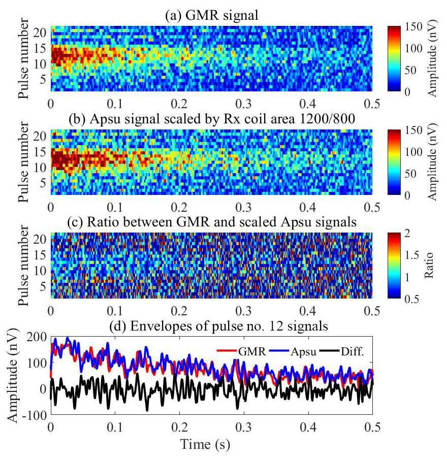
Figure 10 Data space comparison between the commercial GMR instrument and our Apsu receiver. (a) Data space of GMR results. (b) Data space of Apsu results after being scaled to the GMR signal by the area-turn factor of 1200 ∕ 800. (c) Ratio of the GMR and the Apsu signals. (d) Envelopes of the pulse no. 12 NMR signal from the two instruments and the difference.

The signals recorded by two Rx instruments (GMR, Apsu) were processed with the same procedures: band-pass filtering with a 500 Hz bandwidth, power line harmonics subtraction with the model-based method, quadrature detection, and stacking (Müller-Petke et al., 2016). Apsu data are further scaled by the 1200 ∕ 800 ratio of the Rx coils area-turn product. The comparison of the extracted data space from the two instruments is shown in Fig. 10. The initial signal amplitudes recorded by Apsu and GMR are higher than 100 nV within pulse numbers 10–15 (yellow zone) and are smaller than 50 nV in other pulse numbers (blue zone). Figure 10c shows the ratio between the Apsu and GMR signal amplitudes for each point in the data space. The ratios are close to 1 in the region with a strong signal level showing that the two instruments measure the same signal. Outside the region, the ratio is highly varying as these points in the data space contain no signal but only random noise, uncorrelated between the two receiver systems. Figure 10d shows the envelopes of the Apsu (blue) and GMR data (red) and their difference (black) from pulse number 12. The GMR and Apsu envelopes are effectively coincident, decaying from 180 nV with the same relaxation rate. The difference between the two envelopes is random noise, and no signal residual is visible. The same behavior is found in the other pulse moments.

An analysis of the noise in the data sets from the two instruments showed that externally coupled noise is the main component in both cases. The Rx coils for GMR and Apsu overlapped, making the noise levels in the two data sets almost similar, and the small differences can be ascribed to the dissimilarities in receiver bandwidth of the two instruments.

5.2 Effective dead time

The effective dead time consists of instrument dead time and filter settling time, during which the NMR signal is transiently distorted. In standard surface-NMR instruments, where the same coil is used for both transmit and receive, the instrument dead time is caused by the switch procedure between the two modes. Apsu continuously samples the Rx coil signals without any switching and the instrument dead time is therefore potentially 0. However, the analog and digital filters affect the early times of the signal, causing transient effects. Apsu uses untuned Rx coil and short settling-time bandpass filters between 1 and 5 kHz, which leads to a filter settling time of 0.42 ms. More filter settling time is added by a subsequent digital signal processing chain where SNR is increased with a digital bandpass filter, e.g., 3.6 ms for a 500 Hz Butterworth filter.

We measured the effective dead time of the receiver system using the data collected at the Schillerslage test site in Hanover, Germany. The results are shown in Fig. 11. In Fig. 11a, the 40 ms long transmitter pulse with a 10 A peak current is shown, along with the real and imaginary NMR envelopes (blue/black). The pulse starts at 51.2 ms and ends at 91.2 ms. After the transmitter shutoff, the pulse current decays to 0 A in 1.8 ms. The NMR envelopes were obtained by stacking 28 records and digital quadrature detection followed by low-pass filtering with a fourth-order digital Butterworth filter with a cutoff frequency of 500 Hz and a settling time of 3.6 ms. To preserve the signal initial phase during filtering, a forward and reverse filter was used. The NMR envelope is easily evident, but an initial transient is also seen. The zoom-in view of the transmitter pulse turn-off in Fig. 11b shows that the transmitter current has dissipated to 0 A at 93.0 ms and that the NMR signal envelopes are distorted by the transients until approximately 97 ms. This gives an effective dead time of 5.8 ms including excitation current decay in agreement with excitation current decaying time and the settling time of the analog and digital filters.

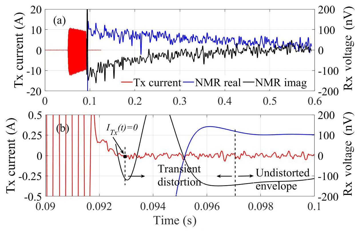
Figure 11 Excitation pulse (red) and the real (blue) and imaginary (black) parts of the surface-NMR signal envelopes. (a) Overview of excitation pulse and surface-NMR signal. (b) Zoom at the early-time signal.

6 Conclusions

We presented a new multichannel surface-NMR receiver system where multiple ApsuRx units each connecting up to three receiver coils are wirelessly connected to an ApsuMaster. The aim of the receiver system is to improve Rx loop deployability and reduce measurement times for multi-coil survey designs in groundwater investigations. We demonstrated that the wireless network performed as designed and remote reference noise cancellation can easily be carried out. In this proof of concept, a distance of 200 m between two receiver coils was used, but the distance can be increased severalfold and multiple reference coils can be employed. We showed that surface-NMR measurements can be performed with the new receiver system and, in particular, that the amplitude and relaxation rate of measured free induction decays are in complete agreement with measurements obtained with a commercial surface-NMR instrument.

The wireless connections between the ApsuMaster and the ApsuRx allow us to place the reference receiver coils in the proximity of identified noise sources. The actual gain in SNR obtained with this new field strategy is heavily dependent on the site-specific noise conditions. The optimization of SNR with the wireless receiver system is a research question which is currently being addressed.