In situ measurements of the ice flow motion at Eqip Sermia Glacier using a remotely controlled unmanned aerial vehicle (UAV)

Measuring the ice flow motion accurately is essential to better understand the time evolution of glaciers and ice sheets and therefore to better anticipate the future consequence of climate change in terms of sea level rise. Although there are a variety of remote sensing methods to fill this task, in situ measurements are always needed for validation or to capture high-temporal-resolution movements. Yet glaciers are in general hostile environments where the installation of instruments might be tedious and risky when not impossible. Here we report the first-ever in situ measurements of ice flow motion using a remotely controlled unmanned aerial vehicle (UAV). We used a quadcopter UAV to land on a highly crevassed area of Eqip Sermia Glacier, West Greenland, to measure the displacement of the glacial surface with the aid of an onboard differential GNSS receiver. We measured approximately 70 cm of displacement over 4.36 h without setting foot onto the glacier – a result validated by applying UAV photogrammetry and template matching techniques. Our study demonstrates that UAVs are promising instruments for in situ monitoring and have great potential for capturing continuous ice flow variations in inaccessible glaciers – a task that remote sensing techniques can hardly achieve.

1 Introduction

Glacial motion is a key process governing the advance or the retreat of glaciers. The accurate recording of ice flow is therefore crucial to calibrate models that can predict the future evolution of glaciers (e.g., Aschwanden et al., 2016). Among them, marine-terminating glaciers usually show fast ice flow (up to several meters per day or even faster) due to buoyant forces with variations at different timescales (e.g., Bartholomew et al., 2012). These range from minute-scale ice flow responses to the collapse of large icebergs (e.g., Murray et al., 2015), to tidally driven hourly-scale variations (e.g., Sugiyama et al., 2015), to daily-scale ice speed-ups induced by rapid change in the subglacial hydrological system (Jouvet et al., 2018), e.g., due to the sudden drainage of a supraglacial lake (Kjeldsen et al., 2014). To continuously capture the dynamics of marine-terminating glaciers, it is therefore necessary to develop methods that can measure their ice flow in high spatial and temporal resolution.

Weekly, monthly, or yearly average ice flow is commonly tracked by satellite images (Moon et al., 2012; Heid and Kääb, 2012), with some data being directly available from general observational programs such as MEASURES (Joughin et al., 2018) or the Greenland Ice Sheet Climate Change Initiative (CCI; http://esa-icesheets-greenland-cci.org, last access: 6 February 2020). Yet revisit times of observation satellites are usually too long to capture variations at daily or subdaily resolution, and in situ validation data are mostly lacking. Alternatively, one can use laser scanning (Pętlicki and Kinnard, 2016) or interferometric radar (Riesen et al., 2011; Lüthi et al., 2016) to increase the temporal resolution of data; however, the spatial coverage of such ground-based instruments remains limited. In recent years, unmanned aerial vehicle (UAV) photogrammetry by structure-from-motion multi-view stereo (SfM-MVS) has been increasingly used for the remote sensing of glacial motion at high spatial resolution (Immerzeel et al., 2014; Ryan et al., 2015; Jouvet et al., 2017; Kraaijenbrink et al., 2016; Benoit et al., 2019; Chudley et al., 2019).

Despite significant improvements in the accuracy of the aforementioned remote sensing methods for ice flow monitoring in recent years, they can not fully substitute in situ measurements. Indeed, in situ accurate GPS (e.g., Sugiyama et al., 2015; Murray et al., 2015) remains necessary (i) for validation purposes, (ii) to perform continuous measurements of ice movements and capture short timescale variability, (iii) to capture glacier vertical motion such as the tidal flexure of ice shelves (Le Meur et al., 2014), or (iv) to capture data whenever the weather prevents the use of remote sensing methods. However, marine-terminating glaciers usually show highly crevassed texture in response to intense tension, making the installation of instruments on ice dangerous and possibly costly (involving helicopter operations) when not impossible.

While UAVs are essentially used as remote sensing platforms in glaciology (Bhardwaj et al., 2016), the latest developments in autonomous navigation and new applications such as delivery drones (e.g., for urgent medical shipping; https://mttr.net/, last access: 6 February 2020) open promising perspectives. Among them, one can cite the deployment of sensors over inaccessible glacial areas, e.g., to measure the motion of marine-terminating glaciers by means of in situ GPSs. Note that McGill et al. (2011) used UAVs to drop GNSS receivers on an iceberg in order to track its drift. While drops by UAV do not present major technical challenges if they occur at a safe distance from the ground, landing a UAV remotely and smoothly over an unknown and inaccessible terrain is much more complex. UAV manually controlled landings within a short distance to the pilot were performed recently to sample ice from an iceberg and from the sea ice (Carlson et al., 2019). To our knowledge, remote landings on ice without direct visual control have never been attempted before, especially over a highly crevassed glacier.

In this proof-of-concept paper, we report the outcomes of the first-ever use of a UAV for in situ sensing of glacial motion. In July 2018, we landed a quadcopter UAV on Eqip Sermia Glacier, West Greenland – a highly crevassed and fast-moving tidewater glacier – and measured the ice motion for more than 4 h thanks to an onboard differential GNSS receiver. In the meantime, we performed traditional UAV photogrammetry over the glacier and processed the resulting ortho-images by template matching in order to cross-check the ice motion record with another well-established technique. This paper is structured as follows. First, we shortly describe the study site (Sect. 2) and provide technical details about the two measurement methods we used: (i) the traditional remote sensing method by UAV photogrammetry (Sect. 3) and (ii) the new in situ method by a UAV-carried GNSS receiver (Sect. 4). Then, we compare the results given by the two methods in Sect. 5 and make recommendations in Sect. 6 for improving the reliability of our approach in the future.

2 Study site

Eqip Sermia Glacier (69^∘48^′ N, 50^∘13^′ W) is a marine-terminating glacier located in the west of the Greenland Ice Sheet (Lüthi et al., 2016); see Fig. 1a. The glacier discharges into the ocean through a 3–4 km wide calving front lying over shallow bedrock, where it features fast ice flow up to 14 m d⁻¹ and frequent calving activity. Due to its intense dynamics, Eqip Sermia is extremely crevassed and mostly inaccessible for in situ sensing. In July 2018, field measurements were carried out for 10 d to remotely monitor the ice dynamics and the calving activity of Eqip Sermia Glacier by terrestrial radar interferometry and UAV photogrammetry.

Figure 1 Ortho-images (a, c, e), velocity field (b), DEM (d), and aerial picture (f) of Eqip Sermia Glacier. (a) Ortho-image processed from UAV images taken during the 11 July large-scale reconnaissance flight together with a map of Greenland (source: Wikimedia Commons) indicating the location Eqip Sermia Glacier by a star. (b) Horizontal ice velocity field inferred by template matching of the ortho-images of the 6 and 11 July flights; (c) 11 July ortho-image around the landing site; (d) 11 July DEM around the landing site; (e) 11 July detailed ortho-image showing the targeted and the achieved landing sites. The position of the achieved landing site was corrected to account for the displacement of ice between 11 and 13 July. Contour lines (20 cm intervals) were drawn to reflect the local topography of the glacier. (f) Example of FPV image used by the UAV operator to adjust the touching point during the landing stage. Two of the four spikes installed under the legs of the UAV are visible on the top left and top right corners (red circles).

3 Remote sensing method

Before landing our quadcopter UAV on the glacier for measuring in situ the ice flow motion (Sect. 4), we performed photogrammetrical UAV flights to produce ortho-images and digital elevation models (DEMs) of Eqip Sermia Glacier, identify an appropriate landing area, and make an initial estimate of the ice flow. For that purpose, we closely followed the approach described by Chudley et al. (2019) and Jouvet et al. (2019). We briefly describe the method in this section and refer to Jouvet et al. (2019) and its Supplement for more details.

3.1 UAV equipment

As a UAV for photogrammetrical flights we used a 2 m wide fixed-wing Skywalker X8 equipped with a Sony α6000 camera described by Jouvet et al. (2019). For inaccessibility reasons, we did not install any ground control points (GCPs) on the sides of the glacier. To ensure an accurate georeferencing of the photogrammetrical results, we used the direct method described by Chudley et al. (2019); i.e., the camera location of each picture was determined using an onboard differential carrier-phase GNSS receiver (the same as described in Sect. 4.2), which can deliver relative centimeter accuracy when combined with a second one (called the base station) fixed on the ground.

3.2 Surveying missions

In total, we performed three large-scale surveys (approximatively 50 km²) of Eqip Glacier on 6, 8, and 11 July. For each flight, the UAV was programmed to fly autonomously along parallel lines covering the terminus of the glacier and about 550 m above the glacier. The UAV collected overlapping pictures with a ground sampling distance (GSD) of 15 to 20 cm as well as an overlap of 95 % in the flight direction and 75 % in the cross-flight direction (Jouvet et al., 2019). On 11 July, we performed an additional low-altitude flight to refine the resolution by a factor of ∼4 (i.e., GSD ∼5 cm) over a zone of interest, which encompassed the future landing area of the quadcopter UAV (Sect. 4 and Fig. 1c, d, and e).

3.3 SfM-MVS photogrammetry

The images collected during the surveying flights were processed by structure-from-motion multi-view stereo (SfM-MVS) using Agisoft PhotoScan software (http://www.agisoft.com/, last access: 6 February 2020) to generate ortho-images and DEMs with a resolution of 25 and 50 cm, respectively (Fig. 1a). As Chudley et al. (2019), we used GNSS-supported aerial triangulation to georeference the photogrammetrical products in a direct manner without any GCPs. For that purpose, we processed the logs of the carrier-phase GNSS receivers to deliver centimeter-accurate picture locations relative to the base station (Sect. 4.2), the absolute locations of which were measured accurately using a differential dual-frequency Leica GPS receiver. The resulting georeferencing accuracy of the ortho-images and DEMs was assessed by Jouvet et al. (2019) against GCPs (only used for error assessment). As a result a horizontal error between 23 and 45 cm was found with a standard mean deviation of 8 cm. This represents an absolute error of about 1–2 pixels, which is slightly less accurate than the error estimate (about 1 pixel) reported by Chudley et al. (2019). Further details on SfM-MVS processing can be found in the Supplement of Jouvet et al. (2019).

Note that it was necessary to perform the SfM-MVS photogrammetry in the field with limited computational resources in order to identify the future landing spot (Sect. 5.1). To deal with this issue, we first processed the full set of images in low quality to look at possible landing sites and second processed the neighborhood of possible sites with the highest quality.

3.4 Glacier velocity derivation

Once the ortho-images and DEMs are obtained, we used the MATLAB toolbox ImGRAFT (http://imgraft.glaciology.net/, last access: 6 February 2020) to derive ice flow horizontal velocities by template matching (Messerli and Grinsted, 2015) from ortho-images of 6, 8, and 11 July; see an example in Fig. 1b. Further details can be found in the Supplement of Jouvet et al. (2019).

4 In situ method

4.1 UAV equipment

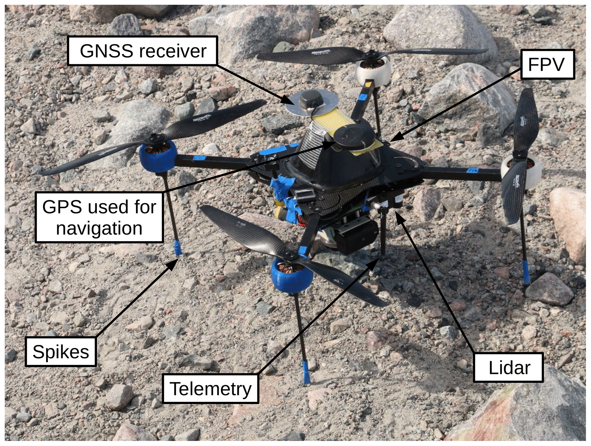
UAV flights for in situ measurements of the ice flow motion were conducted using a customized version of the Enduro (https://droneshop.biz/; last access: 6 February 2020; Fig. 2), which is a quadcopter featuring low-Kv motors, long propellers, and high battery capacity to maximize flight duration. Our UAV was equipped with the Pixhawk 2 open-source autopilot (https://pixhawk.org/, last access: 6 February 2020) running on arducopter firmware (http://ardupilot.org/ardupilot/, 6 February 2020). The latter allows several modes, from manual to fully autonomous flights, that follow a pre-programmed mission script stored in the autopilot. For our application, we equipped our UAV with the rangefinder PulsedLight LIDAR-Lite to estimate the distance to ground accurately and allow for smooth autonomous landings, a first-person view (FVP) with an onboard pointing-down camera to give the UAV operator a real-time view of the ground, and long-range telemetry and remote-control receivers. The UAV was powered by two lithium polymer batteries (240 Wh in total). In this configuration, the power consumption of the UAV varies from 250 to 500 W when flying, allowing for roughly 30 to 60 min of flight time according to the conditions met and the distance traveled. In our case, the amount of time necessary to fly from the UAV operator to the landing site and return was less than 8 min. However, the batteries were also used to power the UAV instruments and an extra GNSS receiver (see Sect. 4.2) while recording the ice motion. To save energy during the measurements, a remote-controlled switch was installed to shut down unnecessary instruments such as the first-person view (FPV) and the lidar shortly after landing. In this saving mode, the UAV consumes ∼5 W. Finally, spikes were installed under the four legs to prevent the platform from sliding over the ice (Figs. 1f and 2).

Figure 2 The Enduro quadcopter UAV that landed on Eqip Sermia Glacier.

4.2 Differential GNSS receiver

The antenna of a second GNSS receiver to measure the ice motion was installed on the UAV next to the antenna used for navigation (Fig. 2). Here we used the single-frequency Emlid Reach receiver (https://emlid.com/reach/, last access: 6 February 2020), which logs carrier-phase data in order to facilitate high positioning accuracy. Note that the GNSS receiver antenna was installed on an aluminum plate to filter reflected waves from downward. Key advantages of the Emlid Reach receiver are the low cost (about USD 300), the light weight (20 g), and the low power consumption (∼1.2 W). Note that a dual-frequency receiver like the Piksi Multi (https://www.swiftnav.com/, last access: 6 February 2020) could have been considered as an alternative to the Emlid Reach for higher positioning accuracy, but with notably higher cost and power consumption.

For data processing in differential mode this receiver (“rover”) works in combination with a second one (“base”), which is fixed on the ground. Differential carrier-phase positioning yields centimeter accuracy (relative to the base station) as long as the distance between the two (base and rover) remains under 10 km, the differential ionospheric delay being negligible for such a small distance (Chudley et al., 2019). Although the Emlid receiver can be used for real-time kinematics (RTK) (i.e., providing the centimeter-accurate position of the UAV in real time), we used it only in post-processed kinematic (PPK) mode for simplicity; i.e., we downloaded the log files of the rover and the base station once the measurements were completed and processed them afterwards via the open-source software RTKLIB (http://www.rtklib.com/rtklib.htm, last access: 6 February 2020).

To assess the positioning accuracy, we performed a static test by leaving the UAV immobile on the ground in the vicinity of the base station for approximatively 6.5 h on a stable off-glacier area and monitored the variability of its position over time (Fig. 3a). We found that 95 % of the recorded positions (after differential processing) were less than 1.1 cm horizontally and 1.6 cm vertically from the mean values. In what follows, we interpret these numbers as the positioning accuracy of our measurement instrument. This accuracy is more than 20 times better than the georeferencing accuracy of photogrammetrical products (Sect. 3.3). As the UAV was lying near the base station in the static test, the positioning inaccuracy induced by the distance between the rover and base was not tested. However, this distance never exceeded 1–2 km in the dynamical test (Sect. 5.3), which is far under the recommended 10 km maximal distance (Chudley et al., 2019).

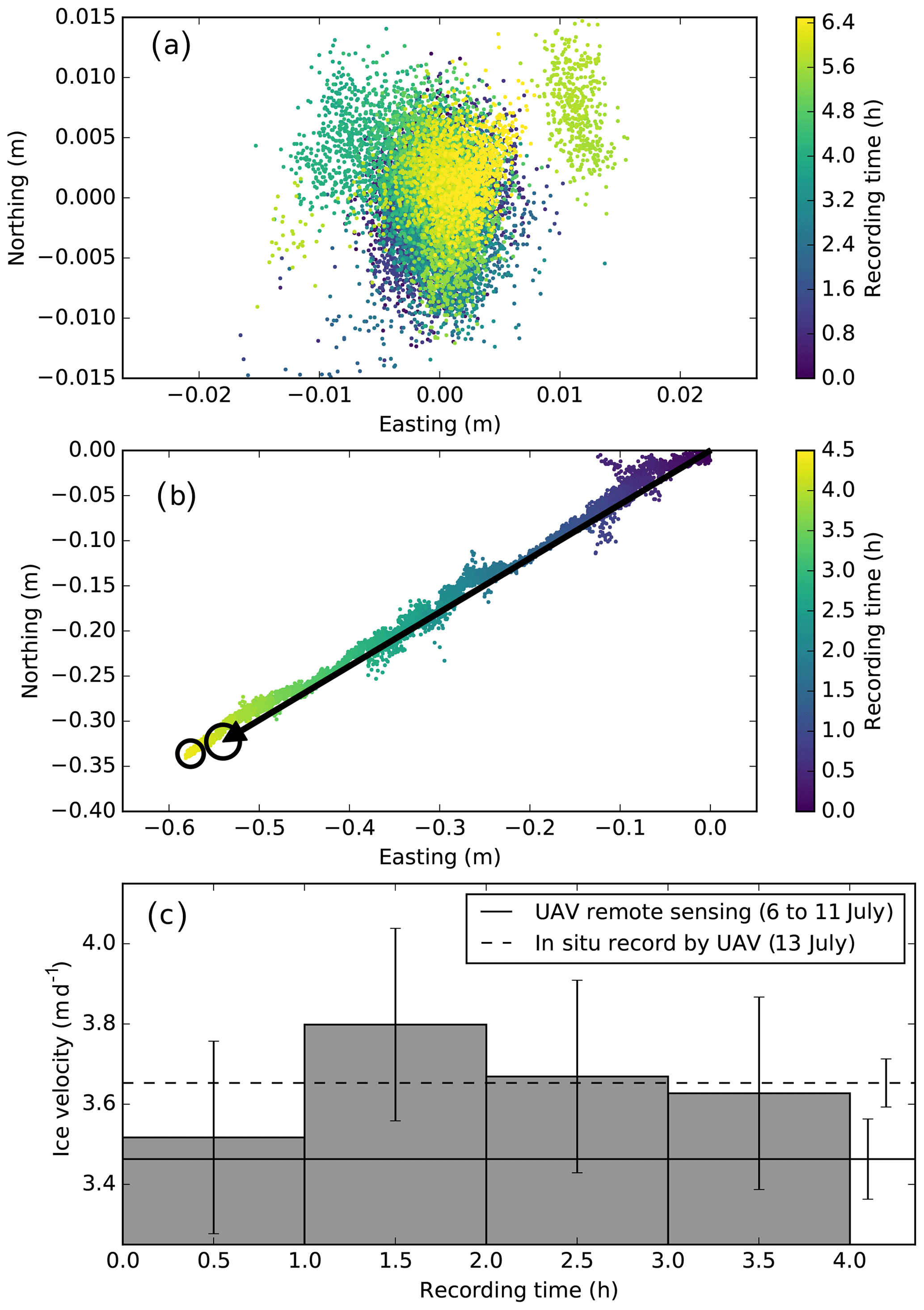
Figure 3 (a) Processed horizontal positions during the static test of our differential GNSS receiver relative to the mean position. (b) Processed horizontal positions of the quadcopter UAV while measuring the ice flow at Eqip Sermia Glacier relative to the landing position on 13 July. The arrow shows the ice displacement vector estimated by SfM-MVS photogrammetry and template matching between 6 and 11 July, but rescaled over the recording time for comparison purposes. The circles indicate the intervals of confidence from both results. (c) Velocity of ice at the recording site every hour determined from 1 h window average positions. The continuous and dashed straight lines indicate the average ice flow motion over the entire recording time and the one inferred by template matching and SfM-MVS photogrammetry from 6 to 11 July, respectively.

5 Results

5.1 Identification of the landing spot

Beyond the scientific relevance, a suitable site to land the quadcopter UAV and to measure the ice motion must fulfill the following requirements: (i) be sufficiently flat to prevent the UAV from turning over and (ii) be in the line of sight of the operator and less than 2 km away to ensure a reliable connection with the remote controller, telemetry, and FPV (Fig. 4). Due to the fragmented topography of Eqip Sermia Glacier (Fig. 1c and d), few sites met these criteria. We identified our landing site on the middle flow line of Eqip Sermia Glacier and at 1.5 km of the closest glacier margin from the detailed DEM inferred from the 11 July surveying flight (Fig. 1e). As the last photogrammetrical flight and the one in situ measuring the ice flow motion (Sect. 5.2) could not be carried out consecutively, we had to correct the position to account for the ice flow motion. For that purpose, we estimated the ice motion of the selected landing spot by applying template matching (Sect. 3.3) to the large-scale ortho-images from 8 and 11 July.

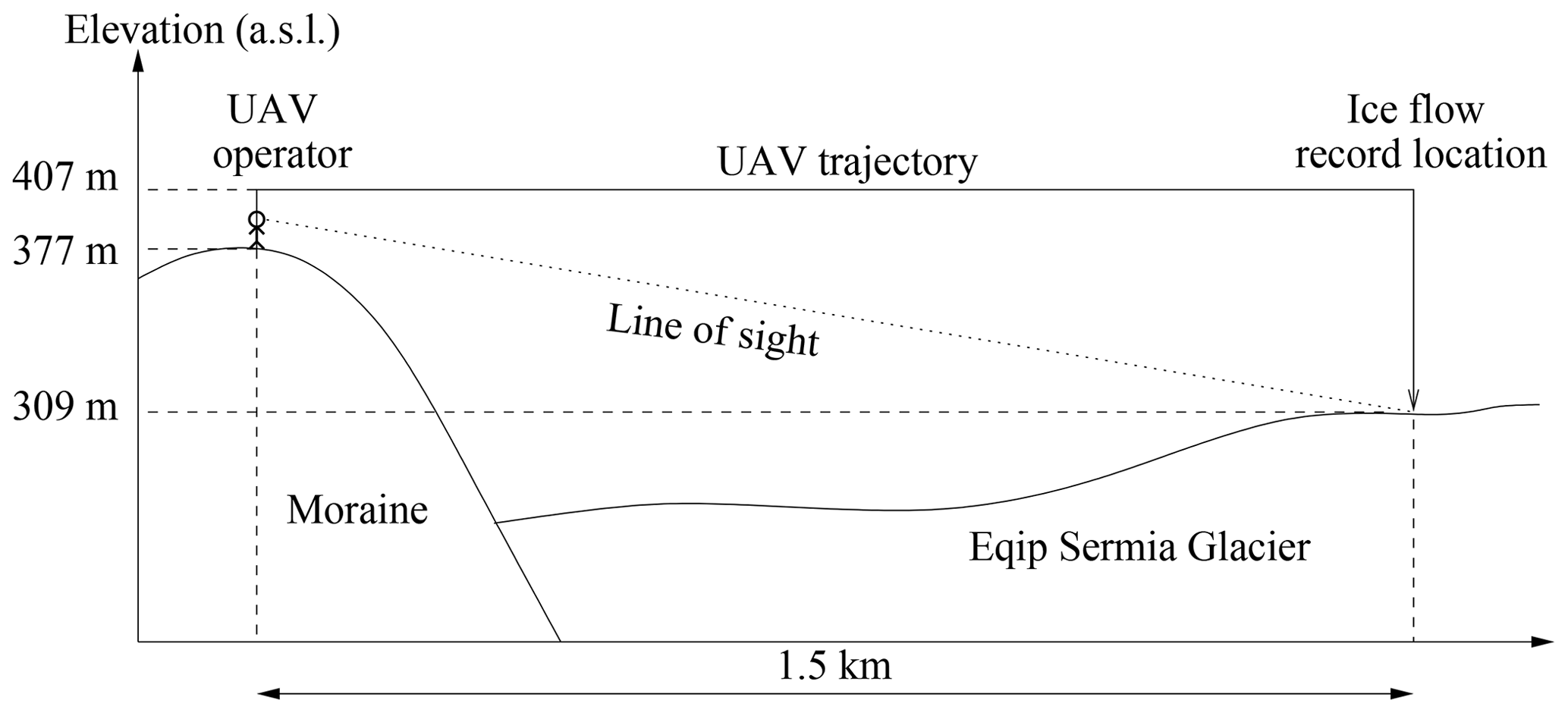
Figure 4 Trajectory of the UAV from the glacier margin to the selected site for in situ measurements of the ice flow.

5.2 Landing on Eqip Sermia Glacier

On 12 July, we operated the quadcopter UAV in autonomous mode to land at the location selected in Sect. 5.1. The UAV took off at 21:59:30 (local time) with no wind and good weather conditions; it traveled at a horizontal speed of ∼10 m s⁻¹ over a 1.5 km distance and at a 100 m altitude difference from the operator to the landing site (Fig. 4). As the UAV was not capable of landing with high accuracy (the GPS used for navigation was not differential), our strategy was to adjust the trajectory of the UAV manually during the landing stage via the remote controller to fine-tune the touching point in line with the images provided by the FPV (Fig. 1f). As a result, the UAV landed 3:36 min after takeoff approximately 3 m from the targeted landing spot, but over a slope of ∼25 % (Fig. 1e), with the result that the UAV tilted over onto two of its propellers. The UAV was left in this inclined position and the battery voltage was monitored via telemetry to determine the time at which the UAV should return before the battery capacity would no longer be sufficient for the flight back; see Appendix A. After 4.36 h a takeoff was attempted. Unfortunately its tilted position caused the UAV to flip over, and become impossible to salvage. Shortly before this happened, the log files of the extra GNSS receiver were downloaded over Wi-Fi so that the measurements of the displacement of the UAV for the period between landing and the mishap could be retrieved.

5.3 Recorded glacier velocity

The data from the UAV-carried GNSS receiver (once processed with the base station) indicate a horizontal displacement towards the southwest of approximately 70 cm in 4.36 h, i.e., 3.7±0.06 m d⁻¹ approximatively 240^∘ with respect to the north direction, clockwise (Fig. 3b). On the other hand, the remote sensing method (UAV photogrammetry and template matching) shows that the ice here moved by 3.4±0.1 m d⁻¹ in a southwest direction (∼239^∘ with respect to the north direction, clockwise) on average between 6 and 11 July (Fig. 3b). Our error estimates are based on georeferencing errors of photogrammetrical products and the variability found with the two other displacement fields from 6–8 July and 8–11 July. As a consequence, the two methods agree well in terms of magnitude (less than 5 % difference; Fig. 3b). The remaining discrepancy is most likely due to differences in the record periods of each method (diurnal variability). Unlike the magnitude, the ice flow directions are expected to be less variable in time. Therefore, the good match between the ice flow directions of the two methods (one degree of discrepancy) provides a reliable validation.

The key advantage of in situ GNSS receivers is that they can determine the ice flow motion continuously in much higher temporal resolution and with greater accuracy than any remote sensing method. The horizontal accuracy gain factor is on the order of 1–2 GSD, i.e., ∼20 in the present case considering that the accuracy of the in situ and remote sensing methods is close to 1 cm and 1–2 GSD, respectively. To compute the horizontal ice flow velocity, we first averaged the time series of the positioning data to get rid of the noise induced by measured uncertainties. Here we used a mean of a 1 h time window, which corresponds to ∼16 cm of displacement, i.e., 15 times the uncertainty of the differential carrier-phase GNSS-based positioning. The results show that the ice velocity varied from 3.5 to 3.8 m d⁻¹ during the measurement period (Fig. 3c). Furthermore, we found a slight vertical motion of ∼4 cm (not shown) during the same time period, which is close to the estimated error.

6 Recommendations

While the record of ice motion was successful, our strategy to retrieve the UAV safely was not. To understand the causes and make recommendations to improve our method, we analyzed in detail the log files of the UAV autopilot (those recorded by the telemetry) and the positions of the extra GNSS receiver. We found two potential causes of the loss of the UAV: (i) manual inputs during the landing stage via the remote controller were found to be more sensitive than expected, which diminished the ability of the pilot to adjust the touching point from FPV; (ii) although the actual landing site was relatively close to the target (less than 3 m, Fig. 1e), this terrain was steeper than the targeted one and our UAV was not designed to land on such a slope. In the absence of wider, clear, and reasonably flat landing side, it is therefore crucial in the future to improve the landing accuracy. This calls for some improvements of both the method and the platform.

Method-wise, preliminary photogrammetrical flights provided crucial information to identify a suitable landing spot, and we recommend that such flights continue to be performed before attempting any further landing mission. However, we advise against using FPV for manual adjustment of the touching point as it is subject to piloting inaccuracies. Instead, the FPV could be used to verify the position of the UAV relative to topographical features (e.g., crevasses; Fig. 1f) using an ortho-image obtained from a preliminary photogrammetrical flight as a reference. It must be stressed that the FPV alone without any reference – even with a controlled axis of the camera – could not be used to identify the landing site as the images provided by the onboard camera do not reflect the local topography of the glacier's uneven and steep slope surface sufficiently well. As an alternative to FPV for accurate landing, we instead recommend using an RTK-equipped UAV, which uses the second GNSS receiver as we did but obtains the correction from the base station in real time (by contrast, here we used it for post-processing), resulting in highly accurate positioning capability. Using the same base station and GNSS receivers for both the reconnaissance and the landing flight would be another improvement as the method would not require any absolute reference point, the measurement of the location of which introduces some additional error. Furthermore, the two flights (reconnaissance and landing) are better operated consecutively with little delay so as to avoid additional positioning errors when updating the landing location with respect to the ice motion. However, it must be stressed that accurate SfM-MVS photogrammetry is computationally demanding and it can be challenging to perform it in the field with limited computational means. To reduce the needs, we advise first processing in low quality the full set of images to roughly identify the position of possible landing spots and second processing only the immediate vicinity of landing spots in high quality to extract their coordinates accurately.

Platform-wise, we recommend using a flatter design than the one used in the present study (Fig. 2) with a low center of gravity so that the UAV is much less unlikely to turn over. Most importantly, we recommend using guards under each propeller, as these could have saved the UAV from the delicate position experienced here. This first experiment was performed conservatively in terms of energy usage, the high power capacity of our UAV having not been fully exploited (the actual flying time was less than 10 % of its capacity). In fact, we could have let the UAV measure the ice motion for more than 10 h before recalling the UAV, as the capacity at the end of this time would still suffice to power the return flight; see Appendix A. Fully shutting down the UAV with the sole energy use by the GNSS receiver would have reduced the power consumption by a factor of 4 and would have increased the recording time by the same factors. Finally, doubling the battery capacity would be possible but this would result in highly increasing the energy consumption during the flying time period. The distance between the launch and measurement sites is a critical parameter for guiding the choice of platform for such an application. If the flight time is rather short (if the distance and the elevation difference between the recording site and the operator are small), the UAV would be better optimized for payload capacity (i.e., with high-Kv motors, short propellers) by carrying additional batteries and staying longer on the ice. Conversely, a UAV optimized for flight time (as the one used in this study) is better used for long distances (>5 km) and large differences in elevation (>300 m). A platform similar to the one used here, but optimized as recommended, would be able to measure the ice motion for more than 48 h while being operated up to 5 km away in calm and 0 ^∘C conditions, such as those found at Eqip Sermia Glacier.

This initial attempt to measure the ice flow motion in situ using a UAV should be seen as a first step toward a further automatized workflow that aims to increase the number of sampling points. In this perspective, UAVs could be used as a sole means of transportation and deployment of GNSS receivers. Indeed, a single UAV can be used to deploy multiple GNSS receivers on the ice, considering that such a station is about 10 times cheaper than a UAV and can transmit the data to the operator remotely. McGill et al. (2011) used a similar approach to track the drift of icebergs. Furthermore, it is easier to maintain a simple GNSS station made of a receiver, telemetry, and a battery than an entire UAV for longer times on ice (e.g., 24 h). Yet, a key challenge associated with this technique will be the stability of GNSS stations for time periods longer than 1 d as they might turn over due to melt. Therefore, the dropping procedure should be combined with a method to recover or reposition GNSS stations. However, automatization of the retrieval of objects by UAV remains a delicate task and an active domain of research in robotics (e.g., Suarez et al., 2017). With increased monitoring times, the drop and the recovery method would certainly strongly enlarge the pool of applications. For instance, GNSS stations left on ice could capture unpredictable processes such as the dynamics of ice shortly prior to and during large calving events.

7 Conclusions and perspectives

We have tested a new in situ sensing method based on a remotely controlled UAV carrying a differential carrier-phase GNSS receiver to measure the ice flow motion of Eqip Sermia Glacier. As a measurement location, we intentionally chose a heavily crevassed that it is inaccessible, even by helicopter, to demonstrate the potential of our approach. We have validated our new method against an established remote sensing method based on UAV surveying, SfM-MVS photogrammetry, and template matching – the two methods agree well in terms of magnitude (less than 5 % of difference) and even better in terms of directions of the ice flow (Fig. 3b). The in situ method captured the ice flow in much higher temporal resolution and with greater accuracy than the remote sensing method. In the present case the horizontal accuracy gain factor was ∼20.

The approach presented in this study has great potential to measure pointwise the short-term variability in the ice motion of tidewater glaciers, especially in inaccessible regions, providing that the UAV can be operated within less than 5 km of the record point while being in the line of sight. Therefore, it could be used to investigate stick–slip events (Lipovsky and Dunham, 2016), the tidal signal of the ice flow at ocean-terminating glaciers (Sugiyama et al., 2015), or the tidal-induced vertical flexure of an ice shelf, which can provide valuable information about the grounding line position (Le Meur et al., 2014).

Beyond this specific application, the technique developed may be used to deploy other sensors in situ – such as weather or seismic stations (Podolskiy et al., 2016) – over sectors of glacier that are not accessible. In this perspective, the development of fully autonomous systems is key to improving the method reliability and replicability. Having UAVs that can deploy sensors on ice without pilot intervention will allow us to significantly increase the number of sampling points while reducing costs and human risk when compared to current in situ manned methods.

Appendix A: Battery's state of charge

Our UAV and the onboard GNSS receiver were powered by two 6S lithium polymer batteries (22.2 V, 10 Ah in total), which were fully charged at takeoff. In this configuration the voltage was maximal (∼25 V; Fig. A1). The UAV battery monitoring system indicated that the 3:36 min flight consumed approximately 6 % of the battery capacity (i.e., 13.6 Wh of the 222 Wh). As a result, the voltage dropped to 24.5 V after the landing on Eqip Sermia Glacier. During the recording time of the ice flow, the battery voltage was used as an indicator of the state of discharge (Fig. A1). In the case of 6S lithium polymer batteries, 21 V was used as a threshold value to indicate imminent full discharge. If the time evolution of the voltage during the recording period is extrapolated linearly (Fig. A1), the UAV could remain for about 10 h on the ice before reaching 21.5 V, which is enough capacity for the return flight (expected to last ∼3.5 min, the same as the first flight). Under these circumstances, the total consumption would have been roughly 100 Wh (30 Wh flying and 70 Wh nonflying), which is about half the capacity of our two batteries. This below-average performance can be explained by the low temperatures, which must have impacted the battery capacities. Despite uninterrupted sunshine conditions, the UAV remained in the shade after landing and stayed at a location where the temperature was close to 0 ^∘C. For this first experiment, we used a conservative voltage threshold value (23.25 V instead of 21.5 V). As a result, we triggered the takeoff from Eqip Sermia Glacier 4.36 h after the landing (Fig. A1).

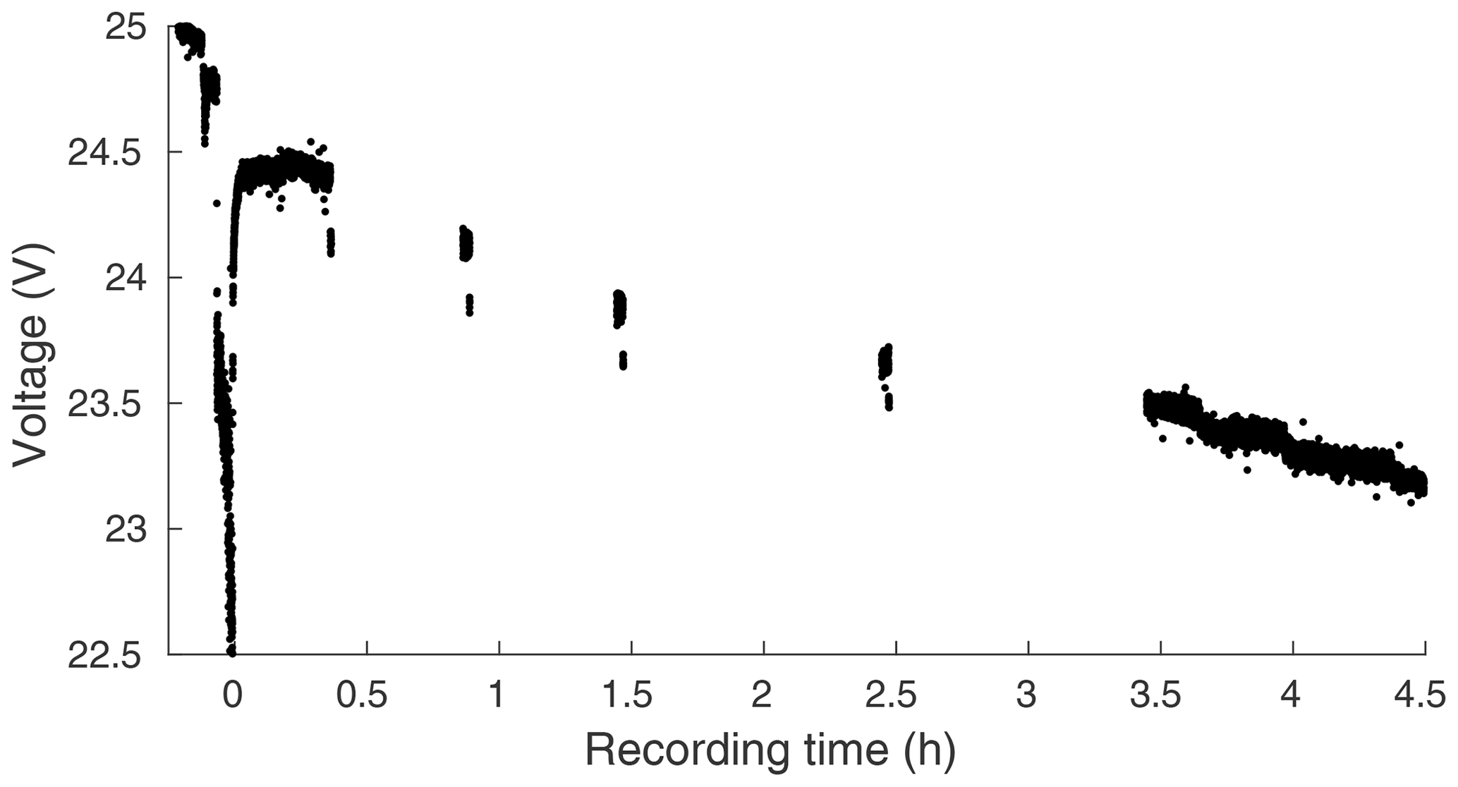
Figure A1 Voltage of the UAV's batteries during and after the flight (t=0 corresponds to the landing time). The flying period (t<0) is characterized by a drop in voltage. The voltage during the nonflying period (t>0) is discontinuous as the data were monitored by telemetry only intermittently. If the time evolution of the voltage was extrapolated linearly, the critical value of 21.5 V would be reached after ∼10 h.