Continuous in situ measurement of dissolved methane in Lake Kivu using a membrane inlet laser spectrometer

We report the first high-resolution continuous profile of dissolved methane in the shallow water of Lake Kivu, Rwanda. The measurements were performed using an in situ dissolved gas sensor, called Sub-Ocean, based on a patented membrane-based extraction technique coupled with a highly sensitive optical spectrometer. The sensor was originally designed for ocean settings, but both the spectrometer and the extraction system were modified to extend the dynamical range up to 6 orders of magnitude with respect to the original prototype (from nmol L⁻¹ to mmol L⁻¹ detection) to fit the range of concentrations at Lake Kivu. The accuracy of the instrument was estimated to ±22 % (2σ) from the standard deviation of eight profiles at 80 m depth, corresponding to ±0.112 mbar of CH₄ in water or ±160 nmol L⁻¹ at 25 ^∘C and 1 atm. The instrument was able to continuously profile the top 150 m of the water column within only 25 min. The maximum observed mixing ratio of CH₄ in the gas phase concentration was 77 %, which at 150 m depth and under thermal conditions of the lake corresponds to 3.5 mmol L⁻¹. Deeper down, dissolved CH₄ concentrations were too large for the methane absorption spectrum to be correctly retrieved. Results are in good agreement with discrete in situ measurements conducted with the commercial HydroC^® sensor. This fast-profiling feature is highly useful for studying the transport, production and consumption of CH₄ and other dissolved gases in aquatic systems. While the sensor is well adapted for investigating most environments with a concentration of CH₄ up to a few millimoles per liter, in the future the spectrometer could be replaced with a less sensitive analytical technique possibly including simultaneous detection of dissolved CO₂ and total dissolved gas pressure, for exploring settings with very high concentrations of CH₄ such as the bottom waters of Lake Kivu.

1 Introduction

Methane (CH₄) is the second-most-important greenhouse gas contributing to the anthropogenic radiative forcing of the atmosphere, and its atmospheric content has risen 2.5-fold since the Industrial Age. During the last decades, significant efforts have been made to better estimate methane contributions of natural and anthropogenic sources to the global atmospheric budget (Kirschke et al., 2013; Saunois et al., 2019). The development of more advanced techniques allowed the recognition of a larger number of sources, which, coupled with the improvements in the modeling, led to continuous rectifications of this budget (Hamdan and Wickland, 2016). In the last 3 decades, natural sources contributed ∼35–50 % of the total global methane emissions, and fresh water constituted one of the largest fluxes after natural wetland and together with geological sources (including seafloor). This highlights the importance and urgency of obtaining a better inventory of the sources of CH₄ reducing the uncertainties of the contributions of aquatic systems (lakes, rivers, estuaries, coastal seas and open ocean) (Ciais et al., 2013). Fast-response instruments for in situ dissolved gas measurements and dynamic profiling can provide the data for a better understanding of the processes of production, transport and transformation.

In this work, a fast-response prototype instrument was deployed for the first time at Lake Kivu, located in East Africa at the border between Rwanda and the Democratic Republic of the Congo. The meromictic character of this lake, defined by a strong stratification of the water, makes deep water strongly decoupled from surface layer because of their difference in density and composition (Schmid and Wüest, 2012). The upper tens of meters (ranging from 65 to 25 m depending on seasons) correspond to the oxic zone, while deeper waters are anoxic and contain large amount of dissolved carbon dioxide (CO₂) and CH₄, with the strongest chemocline situated at 250 m depth (Schmid et al., 2005). Since 1935, several measurement campaigns have been carried out, aiming at quantifying the amount of dissolved CH₄ and CO₂ present in the lake (e.g., Degens et al., 1973; Pasche et al., 2011; Schmitz and Kufferath, 1955; Tassi et al., 2009; Tietze et al., 1980). On the one hand, the presence of those gases constitutes a risk of a catastrophic event such as a gas eruption, which in the past has already occurred in other gas-rich lakes (e.g., in 1984 at Lake Monoun and in 1986 at Lake Nyos in Cameroon; Kling et al., 1987; Kusakabe, 2017; Sigurdsson et al., 1987). On the other hand, dissolved CH₄ represents a potentially important energy resource. Methane extraction would allow compensating for further accumulation of gas at the bottom of the lake and therefore preventing the possibility of a gas eruption. From this field campaign, the maximum total dissolved gas pressure (TDGP) was estimated to be 50±7 % of the hydrostatic pressure at 320 m depth (Bärenbold et al., 2019; Schmid et al., 2019). Meanwhile, extraction has to be performed without destabilizing the stratification of the lake or altering its ecosystem. Regarding the stability of the lake, in Schmid et al. (2005) raised the possibility that dissolved CH₄ in the lake was increasing at a rate of ∼0.5 % per year, with consistent repercussions for the safety of the surrounding population (Schmid et al., 2005). However, from the work of Pasche et al. (2011) as well as the results from this recent field campaign, the hypothesis of a fast increase is today excluded, and the temporal variability appears to be slower than previously expected (Bärenbold et al., 2019; Boehrer et al., 2019; Schmid et al., 2019). In the future, regular monitoring of the lake is required to estimate the CH₄ and CO₂ budgets as well as their temporal variability, using reliable, fast and easy-to-use techniques. For a more precise estimation of the dissolved gas concentration, intercomparison between different sensors and methods is required, as conducted and presented in this work and in the even more comprehensive results from the entire intercomparison campaign (Bärenbold et al., 2019; Boehrer et al., 2019; Schmid et al., 2019). A fast-response sensor like the one proposed here could also be highly useful for estimating methane fluxes from the water surface and their spatial and seasonal variabilities.

In this work we report a successful deployment of the Sub-Ocean sensor in a very different setting, highlighting the reliability and adaptability of the technique to different aquatic environments. Advantages and drawbacks of the technique are highlighted in the discussion section in comparison with other methods deployed during the same campaign: water sampling followed by laboratory gas chromatography (GC) analysis (Boehrer et al., 2019) and online water pumping followed by on-site mass spectrometry analysis (Brennwald et al., 2016). These results are not reported here as they focused on the concentrations in the deep waters (Bärenbold et al., 2019; Schmid et al., 2019).

2 Materials and methods

2.1 The Sub-Ocean instrument

The optical instrument used in this study is based on the OF-CEAS technique (optical-feedback cavity-enhanced absorption spectroscopy) (Morville et al., 2003, 2014) developed for trace gas sensing. The dissolved air from the extraction unit (Fig. 1) is continuously pumped toward the optical cavity of the spectrometer. The internal volume of the cell is less than 20 cm³ and provides sample residence times < 30 s for optimal running conditions (compromise between the cell pressure and the total gas flow).

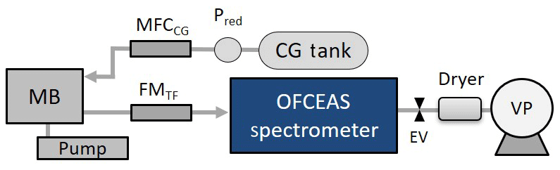
Figure 1 A schematic of the Sub-Ocean sensor. MB is the membrane block where the gas extraction occurs. Water circulates at the membrane using a submersible pump. The carrier gas (CG) flow is controlled by a mass flow controller (MFC_CG), and the flowmeter FM_TF is used for monitoring the total gas flow. The low pressure on the optical spectrometer is provided by a vacuum pump (VP) and an electronic valve (EV). P_red is a pressure reducer. A silica gel dryer is placed before the VP to trap water vapor.

Extraction of dissolved gases from water is performed using a silicon polydimethylsiloxane (PDMS) membrane. The extraction technique does not rely on gas equilibration across the membrane, but, in order to achieve fast response, the dry side of the membrane is maintained at low pressure while continuously flushing it with dry zero air (Triest et al., 2017). The pressure at the dry side controls the total flow of dry and wet air through the membrane, and the system is designed to keep this pressure constant. While the spectrometer operates at about 20 mbar, the pressure at the dry side of the membrane is maintained at about 30 mbar.

A full description of the in situ membrane inlet laser spectrometer instrument (Sub-Ocean), together with the experimental setup used for laboratory calibrations can be found in Grilli et al. (2018) and Jansson et al. (2019). In order to adapt the instrument to the high concentrations of dissolved CH₄ expected in Lake Kivu, the absorption spectrum of the optical spectrometer was set away from the strong CH₄ rotational–vibrational transitions, more precisely at 2238.5 nm, where concentrations inside the optical cavity may reach up to 1.5–2 % CH₄ in air before optical saturation (equivalent to the absorption of 10⁻⁵–10⁻⁶ cm⁻¹). Above this absorption, the transmission signal at the maximum of the peak of absorption becomes too weak and the optical feedback to the laser, required by the optical method, is no longer strong enough to lock the laser frequency for a period of time close to the cavity free spectral range. This leads to narrower cavity modes and to a failure in correctly retrieving the absorption features. A stainless-steel membrane block (MB) was equipped with two 10 µm thick PDMS membranes of 56 mm diameter mounted face to face. The thin-film membranes were mounted on porous bronze frits of 3 mm thickness (Poral, grade 20), providing mechanical strength for the membrane under high hydrostatic pressure. A schematic of the membrane block can be found in the supplementary information of Grilli et al. (2018). For this campaign, in order to increase the dynamic range of the measurements, one of the two membranes was replaced with a gas-tight Teflon film. This increased the dilution factor by decreasing the flow of the permeating gas with respect to water vapor and carrier gas flow, but it degrades the precision of the measurements due to the low dry gas flow through the membrane. A picture of the instrument and the assembly taken during the campaign is shown in Fig. 2. The main (central) pressure tube (140 cm long, 28 cm diameter) is mounted on a metal frame. The membrane block at the bottom is connected with a submersible water pump (Sea-Bird Electronics, SBE 5T) providing a flow of 0.8 L min⁻¹ along the membrane. A 1 L carrier gas (CG) tank containing dry zero air at a pressure between 2 and 40 bar, depending on the suitable autonomy, is attached on the frame and connected to the instrument via a 1∕8 in. stainless-steel tube. A subsea battery (Seacell, STR) was mounted on the metal frame, providing up to 12 h of continuous operation. An independent CTD (temperature, conductivity and dissolved oxygen; Sea & Sun Marine Tech, CTD-60) was also attached to the frame for depth, temperature, conductivity and dissolved oxygen measurements. For an operation where the instrument is powered through an electromechanical cable the autonomy will be limited by the storage of the dry gas inside the instrument housing. For fast-response measurements, at maximum carrier gas flow of 6 mL min⁻¹ is required, corresponding to an autonomy of 24 h, whereas without the use of carrier gas the autonomy will stretch to 90 d since most of the gas flow will be composed of water vapor that is trapped before the vacuum pump by the silica gel dryer (however, the long-term deployment may be limited by the capability of the silica gel).

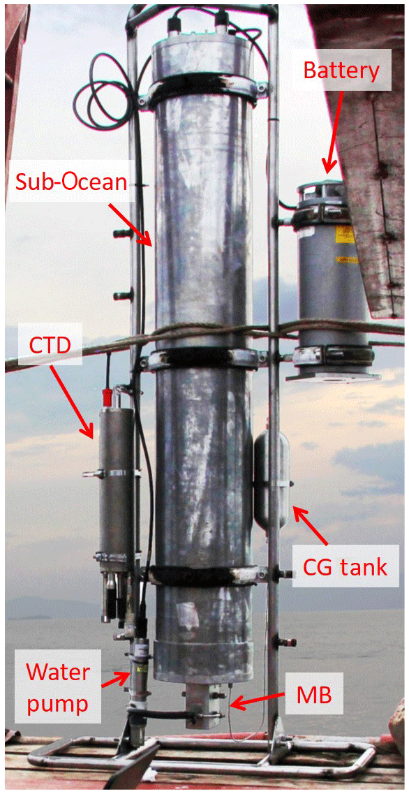
Figure 2 A picture of the Sub-Ocean instrument and the full assembly. The sensor is mounted on a metal frame. The main tube at the center is 150 cm long and 28 cm in diameter. The membrane block (MB) at its bottom is connected to the water pump to ensure a constant flow of water against the membrane. The carrier gas (CG) tank is attached to the metal frame and connected with a 1∕8 in. stainless-steel tube at the instrument. An STR battery pack and a CTD sensor were also attached to the metal structure. The total weight of the assembly is 120 kg with about −50 kg of buoyancy.

The embedded spectrometer continuously measures the gas composition at 10 Hz, while the response time of the sensor during the campaign, expressed as τ₉₀, was ∼10 s At a lowering speed of ∼6 m min⁻¹, the vertical resolution is 1 m. From the composition of the dissolved gas the instrument can indirectly estimate the amount of N₂. This requires knowing TDGP, pCO₂ and pO₂, which were not measured by the Sub-Ocean probe and rely on other sensors. The partial pressure of N₂ can then be estimated as pN₂ = TDGP − pCH₄ − pCO₂ − pO₂.

2.2 The HydroC CH₄ commercial instrument

In situ discrete measurements of dissolved CH₄ at five different depths along the upper 150 m of the water column were performed using a commercial equilibrium-based underwater sensor, the Contros HydroC^® HP sensor. The dissolved gas diffuses from the liquid through a thin film composite membrane into an internal gas cell. Therein, the total dissolved gas pressure and the partial pressure of CH₄ gas are measured by a pressure sensor and a non-dispersive infrared spectrometer, respectively. The HydroC^® CH₄ HP sensor is similar to the HydroC^® CO₂ sensor presented in Fietzek et al. (2014), except for the absence of an internal zeroing system and a CH₄-specific fixed narrow-band spectral filter from 3.3 to 3.4 µm. The sensor was calibrated in October 2012 and November 2015 by the manufacturer. The calibrations were made using a specially designed pressure chamber with fresh water brought to pressure using compressed target gas. Three standard gas mixtures of CO₂, CH₄ and N₂ (100 % pressure N₂; 50 % pressure CH₄ and 50 % pressure CO₂; 100 % pressure CH₄) were used to equilibrate the water volume along a gas pressure gradient (five–six points) from 1 up to 30 bars and partial pressures of CH₄ from 0.5 to 18 bars. The calibration results showed the absence of a significant drift of the sensor (< 3 % within the Lake Kivu gas concentration range) between the October 2012 and November 2015 calibrations. Also, several CH₄ profiles were carried out in Lake Kivu from 2016 to 2018 using the HydroC^® CH₄ HP sensor, and the repeatability of the observed CH₄ partial pressures was 3.8 % (2σ) below the main density gradient. However, the calibration curve as a function of the methane concentration was determined by using three points (0, 50 and 100 % CH₄), and because of the nonlinear behavior of the detection system a systematic error could be present, but it should not exceed 10 % (manufacturer personal communication, KM Contros, 2019).

The HydroC^® CH₄ HP system was mounted on a SeaBird 19plus V2 SeaCAT CTD profiler equipped with a SBE 43 dissolved oxygen sensor and a SBE 18 pH sensor. Calibrations of the SeaBird sensors were performed following manufacturer instructions. Water circulation in front of the membrane was provided by a SeaBird 5T pump, ensuring a continuous and homogeneous water flow at the membrane. A zero calibration of the system was made daily before each deployment using surface waters. The sampling rate was 1 Hz. The steady state of the sensor was generally reached within 40 min, and real-time data communication using an electromechanical cable allowed the waiting time at each depth to be adjusted accordingly. In all cases, the waiting time for each depth never exceeded 1 h. The retained partial pressure of CH₄ is the average for the last 5 min of the equilibration curve.

2.3 Calculation of dissolved CH₄

Both the Sub-Ocean and the HydroC^® HP sensors measure CH₄ in the gas phase, and raw data are expressed as the concentration of CH₄ with respect to the total amount of dry gas permeating the membrane. For the Sub-Ocean system, the concentration of CH₄ in the dry gas downstream from the membrane, [CH₄]${}_{\mathrm{g}}^{\prime }$, can be expressed with respect to the expected concentration of the gas in the headspace which would be in equilibrium with the water sample, [CH₄]_g. In Eq. (1), Pr are the membrane permeability coefficients for CH₄ and X (N₂, O₂ and CO₂) reported in Robb (1968) but corrected for their temperature and salinity dependency.

$$\begin{array}{}\text{(1)}& {\left[{\mathrm{CH}}_{\mathrm{4}}\right]}_{\mathrm{g}}^{\prime }={\displaystyle \frac{{\mathrm{Pr}}_{{\mathrm{CH}}_{\mathrm{4}}\cdot {\left[{\mathrm{CH}}_{\mathrm{4}}\right]}_{\mathrm{g}}}}{\sum {\mathrm{Pr}}_x\cdot {\left[X\right]}_{\mathrm{g}}}}\end{array}$$

Concentrations, [CH₄] and [X], are expressed as mixing ratios. Measuring the concentration of water vapor, [H₂O]_g, is required in order to retrieve the dissolved CH₄ concentration, [CH₄]_diss, since water vapor flow will cause dilution of the measured dry gas mixture (as well as the carrier gas flow). This measurement is performed by the OF-CEAS spectrometer embedded in the Sub-Ocean probe, simultaneously with the CH₄ measurement. Precision of the water vapor concentration was ±0.6 % (2σ). [CH₄]_diss is then calculated using the following equation:

$$\begin{array}{}\text{(2)}& {\left[{\mathrm{CH}}_{\mathrm{4}}\right]}_{\mathrm{diss}}^{\prime }={\displaystyle \frac{{\left[{\mathrm{CH}}_{\mathrm{4}}\right]}_{\mathrm{g}}^{\prime }\times f_{\mathrm{t}}}{f_{\mathrm{t}}-f_{\mathrm{CG}}-\left(f_{\mathrm{t}}\times {\left[{\mathrm{H}}_{\mathrm{2}}\mathrm{O}\right]}_{\mathrm{g}}\right)}}\times {\displaystyle \frac{\mathrm{1}}{m_{\mathrm{eff}}}},\end{array}$$

where [CH₄]${}_{\mathrm{g}}^{\prime }$ represents the methane mixing ratio measured by the optical spectrometer; f_t and f_CG are the total- and carrier-gas flow (mL min⁻¹), respectively; and [H₂O]_g corresponds to the mixing ratio of water permeating through the membrane. The denominator term ($f_{\mathrm{t}}-f_{\mathrm{CG}}-(f_{\mathrm{t}}\times [{\mathrm{H}}_{\mathrm{2}}\mathrm{O}{]}_{\mathrm{g}})$) corresponds to the dry flow permeating the membrane. m_eff represents the enrichment factor due to the membrane and corresponds to the quantity $\frac{{\mathrm{Pr}}_{{\mathrm{CH}}_{\mathrm{4}}}}{\sum {\mathrm{Pr}}_x\cdot {\left[X\right]}_{\mathrm{g}}}$ in Eq. (1). Its dependency on temperature and salinity is calculated by running calibrations under various conditions (Grilli et al., 2018). From our calibration, a m_eff of 2.84±0.11 for fresh water at 25 ^∘C and 1.2 bar was calculated. This is in agreement with an expected value of 2.76 calculated from the permeation coefficients reported by Robb (1968).

As reported in Eq. (1) above, this technique requires knowing the main composition of the dissolved gas, in order to account for the different permeation coefficients of the species through the PDMS membrane. This does not represent a problem for most of the ocean and lake settings, where the gas mixture is mainly composed of nitrogen and oxygen, but it requires a more complex analysis for a setting such as Lake Kivu. For the data analysis we assumed a bulk gas mainly composed of N₂, O₂, CO₂ and CH₄. H₂S is only present in bottom water and in a smaller amount with respect to CO₂ and CH₄, and it was therefore neglected here. Oxygen concentrations were calculated from the CTD measurements and converted into partial pressures using Eq. (19) from Sander 2015 (using H^cp of $\mathrm{1.25}\times {\mathrm{10}}^{-\mathrm{5}}$ mol m⁻³ Pa⁻¹ and dln(H^cp) ∕ d(1∕T) of 1500 K).

As mentioned above, concentrations reported so far are expressed in mixing ratio with respect to the TDGP. Therefore, given the TDGP, a value of partial pressure, pCH₄, can be retrieved, which is then converted into dissolved methane concentrations, $C_{{\mathrm{CH}}_{\mathrm{4}}}$, expressed in mol per liter of water. This conversion is performed by considering the solubility of the gas in water under given physical conditions as well as its fugacity. The procedure has been previously described in a scientific report (Schmid et al., 2019). C${}_{{\mathrm{CH}}_{\mathrm{4}}}$ is related to the pCH₄ through the following equation:

$$\begin{array}{}\text{(3)}& C_{{\mathrm{CH}}_{\mathrm{4}}}=K\left(T,S,P\right)p{\mathrm{CH}}_{\mathrm{4}}{\mathit{\phi }}_{{\mathrm{CH}}_{\mathrm{4}}}\left(T,P\right),\end{array}$$

where ${\mathit{\phi }}_{{\mathrm{CH}}_{\mathrm{4}}}$ is the fugacity coefficient – i.e., the ratio between the fugacity of a gas and its partial pressure, which is a function of temperature T, pressure P and gas composition – and K is the solubility coefficient, i.e., the ratio between the dissolved concentration of a gas and its fugacity. The solubility coefficient K (mol L⁻¹ atm⁻¹) of CH₄ as a function of temperature T (K) and salinity S (g kg⁻¹) is calculated using the following equation:

$$\begin{array}{}\text{(4)}& \begin{array}{rl}\ln \left(K\right)& =A_{\mathrm{1}}+A_{\mathrm{2}}\left(\mathrm{100}/T\right)+A_{\mathrm{3}}\ln \left(T/\mathrm{100}\right)\\ & +S\left[B_{\mathrm{1}}+B_{\mathrm{2}}\left(T/\mathrm{100}\right)+B_{\mathrm{3}}{\left(T/\mathrm{100}\right)}^{\mathrm{2}}\right].\end{array}\end{array}$$

The parameters in Eq. (4) are from Wiesenburg and Guinasso (1979).

The solubility coefficients need to be corrected for the local pressure P (bar) at the sampling depth (sum of hydrostatic pressure plus atmospheric pressure), using the following equation (Weiss, 1974):

$$\begin{array}{}\text{(5)}& K\left(P\right)=K{e}^{\left[\frac{\left(\mathrm{1}-P\right)v_{{\mathrm{CH}}_{\mathrm{4}}}}{RT}\right]},\end{array}$$

where R=83.1446 cm³ bar K⁻¹ mol⁻¹ is the gas constant, and ${\mathit{\nu }}_{{\mathrm{CH}}_{\mathrm{4}}}$ is the partial molar volume (cm³ mol⁻¹) of CH₄ calculated from Rettich et al. (1981).

The fugacity coefficients were calculated using the methods described in Ziabakhsh-Ganji and Kooi (2012). A Maple script was provided by the authors, which was transcribed to Matlab code by Schmid (2019). The script calculates, among other things, the fugacity coefficients for CO₂ and CH₄, including the interactions between both gases.

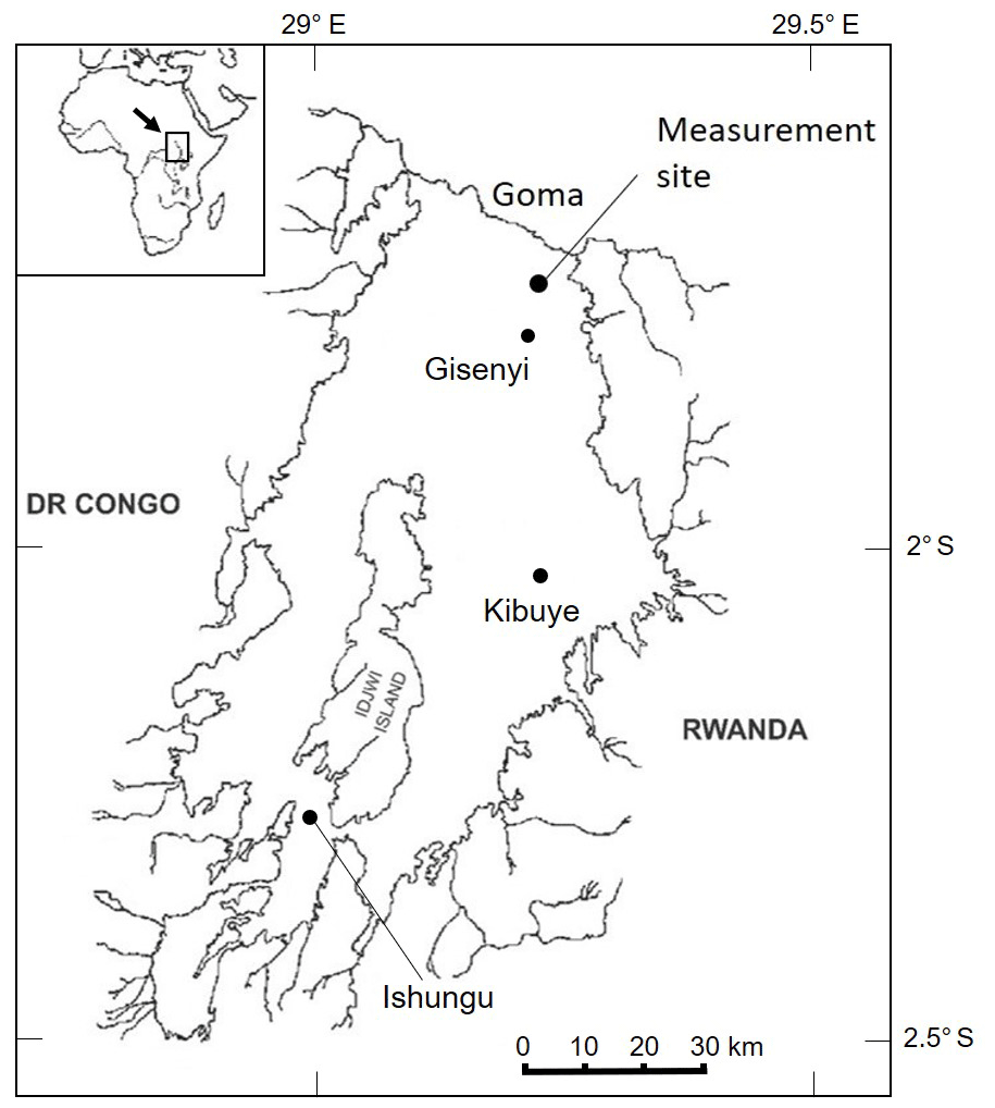
Figure 3 Map of Lake Kivu showing the location of the measurement site. Locations of previous campaigns mentioned in the discussion section are also reported (named Gisenyi, Kibuye and Ishungu).

2.4 The lake and the field campaign

Lake Kivu (2.50–1.59^∘ S, 29.37–28.83^∘ E) located at 1460 m above sea level, has a surface of 2700 km² (of which 2385 km² represents the water cover) and a maximum depth of ∼485 m. The measurement campaign took place from 9 to 13 March 2018 approximately 6 km from Goma and approximately 5 km from Gisenyi/Rubavu at the northern shore of the lake (1.74087^∘ S, 29.22602^∘ E) and near a permanent platform with water depth of 410 m (Fig. 3). During the campaign other types of measurements of dissolved methane and carbon dioxide were performed. The research team from Eawag (Switzerland) analyzed pumped water on the platform using a field mass spectrometer instrument (Brennwald et al., 2016), while a second team from the Helmholtz Centre for Environmental Research (UFZ, Germany) sampled water from a boat and measured the samples by headspace equilibration and GC analysis at the Lake Kivu Monitoring Program (LKMP) laboratory in Rubavu (Boehrer et al., 2019). The Sub-Ocean sensor was deployed from a research boat during 3 d of the campaign – 10, 12 and 13 March – with a total of eight continuous profiles. Measurements with the commercial HydroC^® HP sensor were conducted during the campaign and on 8–11 May at the same location as the Sub-Ocean measurements and over specific discrete depths.

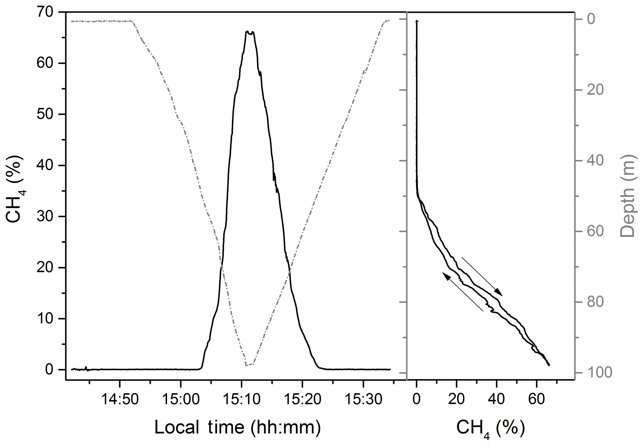
Figure 4 One of the continuous methane profiles recorded by the Sub-Ocean on 10 March 2018. The concentration is expressed as a percentage of CH₄ with respect to the total dissolved gas. The 100 m downward and upward profile was recorded in 42 min. On the right panel the two profiles are superposed, highlighting the reproducibility of the measurement between descent and ascent.

3 Results and discussions

In Fig. 4 an example of a consecutive downward and upward profile of dissolved CH₄ measured by the Sub-Ocean sensor is reported. CH₄ concentrations are expressed as mixing ratio with respect to the total dissolved gas. The sensor was lowered at a speed of ∼6 m min⁻¹, reaching 100 m depth in only 18 min. The response time of the sensor during the campaign expressed as τ₉₀ was ∼10 s, which corresponds to a vertical resolution of 1 m. On the right-hand side, dissolved CH₄ is plotted against depth, showing the reproducibility of the sensor during descent and ascent.

Figure 5 Mixing ratios of individual gas species in the dissolved gas mixture and total dissolved gas pressure. Grey CH₄ lines represent the eight profiles recorded by the Sub-Ocean instrument during the campaign, while the black line is the averaged value. CO₂ data are from Schmid et al. (2005); O₂, temperature and electrical conductivity are from CTD data during the campaign; and N₂ is a concentration profile deduced from the other measurements (TDGP − pCH₄ − pCO₂ − pO₂). The total dissolve gas pressure, TDGP, was measured using the Contros HydroC^® HP sensor (open circles); the black line is an interpolation of the data.

A total of eight continuous profiles (downward and upward) were obtained with the Sub-Ocean instrument during the campaign. They are reported in Fig. 5 together with dissolved CO₂, CTD data (temperature, conductivity and dissolved oxygen) and total dissolved gas pressure (TDGP). For the measurement of CH₄ only one of the eight profiles reached 150 m, while the others were shallower, only covering the uppermost 100 m. The accuracy of the measurement was estimated at 80 m depth, where water mass is well stratified. At this depth, an average concentration of 35.5±7.8 %, corresponding to 508.3±112 mbar of partial pressure and 0.71±0.16 mmol L⁻¹ of CH₄, was calculated, leading to a repeatability of ±22 % (2σ). This relatively large standard deviation can be explained by the large uncertainty in determining the total flow of dry gas permeating the membrane. The value is in agreement with previously observed performances, where an error propagation of ±12 % (2σ) was calculated using two semipermeable membranes (Grilli et al., 2018). The use of only one membrane allowed further increasing the dynamic range of the sensor by diluting the dry gas permeating the membrane. However, in these conditions, a dry gas flow of only ∼0.065 cm³ STP min⁻¹ is delivered by the extraction system. The large uncertainty in this dry flow measurement directly affects the accuracy of the retrieved concentration. The uncertainty represented by the grey lines in Fig. 6 represents the measured variability over the eight vertical profiles from 0 to 80 m and was fixed to ±22 % at larger depths. The CO₂ data are from Schmid et al. 2005 and are calculated from alkalinity and pH measurements. TDGP measurements are discrete measurements at seven different depths measured with the HydroC^® HP sensor which have been interpolated to match the depth resolution of the Sub-Ocean data. The nitrogen (N₂) mixing ratio was retrieved assuming that the main gas is composed of N₂, CO₂, CH₄ and O₂ (pN₂ = TDGP − pCH₄ − pCO₂ − pO₂).

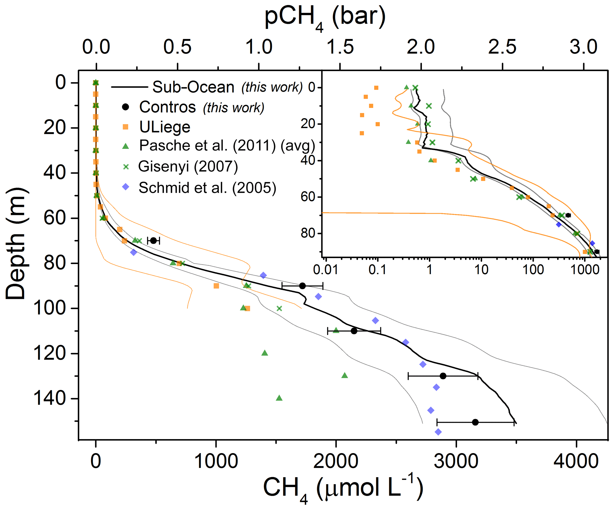
Figure 6 Continuous methane profile of the upper 150 m of water depth in Lake Kivu measured by the Sub-Ocean instrument (black line). Grey lines represent the measured variability over the eight continuous profiles estimated between 0 and 80 m depth and fixed to the estimated uncertainty of ±22 % at larger depths. Black dots are discrete measurements made with the Contros HydroC^® HP sensor at different depths. Error bars correspond to the estimated uncertainty of ±10 %. Orange squares are from the long-term monitoring undertaken by the University of Liege (Roland et al., 2017, 2018) with the corresponding 3σ variability (orange lines). Green triangles are average concentrations from Pasche et al. (2011) from three different campaigns conducted in May 2006 and 2007 at different locations (Kibuye, Ishungu and Gisenyi). Green crosses are data from Gisenyi (2007) from Pasche et al. (2011). Blue rhombuses correspond to measurements from Schmid et al. (2005) in the northern basin using a commercial Capsum Met sensor (Schmid et al., 2005). In the inset a zoomed-in view of the shallow data is presented with a log scale on the concentrations allowing a better comparison of the different datasets.

The molar concentrations as a function of depth for the average continuous profile recorded by the Sub-Ocean sensor and for the discrete measurements obtained with the HydroC^® HP sensor are reported in Fig. 6. A good agreement between the two independent measurements is observed. The measurements were obtained during the same field campaign at the measurement site location near Goma (the two vessels were a few hundred meters away from each other). However, the measurements were not performed simultaneously. In the graph, results from previous campaigns are also reported. Data from the University of Liege obtained during a long-term monitoring campaign of the lake are reported in orange. Data were collected from June 2011 to August 2014 at different periods of the year (both dry and rainy seasons) and at different locations (northern and southern basin) (Roland et al., 2017, 2018). The large variability of these measurements is reported by the orange lines (Fig. 6) defining the 3σ distribution. Data from the works of Pasche et al. (2011) and Schmid et al. (2005) are also reported in green and blue, respectively. The measurements from ULiege and Pasche et al. (2011) were obtained by sampling the water using Niskin bottles and analyzing the dissolved gas in the laboratory by a headspace technique followed by GC analysis. The others (this work and Schmid, 2005) are from in situ measurements. From the data, one can see that below 80 m depth, where the TDGP becomes larger than atmospheric pressure (1.4 bar at 80 m, Fig. 5), a problem due to degassing of the sample collected on the Niskin bottles was observed, leading to an underestimation of the dissolved CH₄. Data from Schmid (2005), which are from a commercial Capsum Met sensor (Franatech), and data from the Contros sensor are a bit lower than the measurements with the Sub-Ocean probe at higher concentrations (and depths), but they still lie within the measurement uncertainties. During the campaign the HydroC^® HP sensor also showed good agreement with the other discrete techniques (on-site mass spectroscopy and discrete sampling followed by GC analysis) between 150 and 250 m, while at greater depths the HydroC^® HP values were lower by ∼12 % (Schmid et al., 2019). This may be due to a problem of calibration of the sensor at high hydrostatic pressures, but it requires further investigations to be confirmed. Regarding the Capsum Met sensor, no information about the calibration of the sensor was found; therefore no further discussion can take place.

Surface measurements performed by the Sub-Ocean instrument lead to average concentrations of 0.59±0.03 µmol L⁻¹ and 0.72±0.14 µmol L⁻¹ over the upper 10 and 30 m, respectively. Those values sit at the higher edge of the observed average seasonal concentrations, which span from 0.008 to 11 µmol L⁻¹ (Roland et al., 2017, 2018 and more recent unpublished data from the same authors). Despite the large seasonal and spatial variability, our results are in good agreement with those from Pasche et al. (2011), which were obtained at a similar time of the year but at different locations (May 2006 and 2007 in Kibuye, Gisenyi and Ishungu). A stronger similarity can be found with the dataset from the same location (Gisenyi, 2007) in the northern basin. CTD measurements (Sea & Sun Marine Tech, CTD-90M) performed a few months prior to the campaign at the research platform (Fig. 7) confirmed a typical behavior of the lake stratigraphy while going from a dry into a rainy season (Roland et al., 2017) and therefore justified the high concentrations measured in this work. The lake was mixed down to at least 50 m depth during the previous dry season and started to stratify in mid-December, leading to a 25 m depth seasonal thermocline. Below the thermocline, O₂ was rapidly consumed by mineralization of organic matter and oxidation of reduced compounds (e.g., methane and ammonium) diffusing upward. By the end of February, O₂ supplied at these depths during the previous dry season had completely vanished. Then, in the first half of March, a mixing event occurred down to about 35 m depth, favoring the mixing between anoxic water (35–25 m depth), enriched in dissolved CH₄, and surface water. From the top 10 m layer temperature profiles reported in Fig. 7 one can see that by 22 March the temperature slope disappeared, supporting the occurrence of the water mixing. Unfortunately, the reasons for this mixing event are still unknown. Meteorological records from December 2017 to March 2018 do not indicate high-wind-speed, low-temperature or low-relative-humidity events that could support our observations. Comparing the second half of February to the first half of March, average temperatures decreased by 1 ^∘C (from 21.2 to 22.2 ^∘C) and average precipitations increased by a factor of 2, with peaks up to 7.6 mm of rainfall on 6 March. As reported by Rooney et al. (2018), rain may have a cooling effect on the lake surface by lowering the near-surface air temperature and inducing a convective mixing of the lake surface layer. Finally, CH₄ concentration in the surface layer may depend on biogeochemical processes such as methanotrophy. Further investigations are therefore required to better understand the dynamics of the surface layer of the lake at this period of the year.

Figure 7 CTD (conductivity at 25 ^∘C, temperature and dissolved oxygen) data obtained a few months prior to the campaign. The black lines correspond to the conditions during the field measurements (^*). The O₂ profiles highlight how the mixing layer extended down to 50 m depth during the previous dry season. From mid-December, the lake started to stratify at 25 m, while at the beginning of March the oxic layer increased down to 35 m depth.

This type of fast-response sensors could be used to better investigate the fluxes of CH₄ (or other greenhouse gases) from lakes, oceans, rivers and other water bodies. In this campaign, only a specific location at 5 km from the coast with 410 m of water depth was investigated. The amount of CH₄ at the surface may strongly depend on the water depth, i.e., on the distance of the sediment to the surface, as well as on the horizontal distance from the shore and littoral sediments (DelSontro et al., 2018b). A fast sensor would allow following the spatial distribution of dissolved gases at the surface layer, as well as its variability over the seasons. This would help to better constrain the greenhouse gas emissions in the face of global change (DelSontro et al., 2018a). Beside the advantages of the Sub-Ocean probe providing in situ, continuous and fast measurements, some drawbacks of the technique can be identified: (i) the instrument was designed for measuring background concentrations in the ocean (∼ nmol L⁻¹), while Lake Kivu reaches ∼18 mmol L⁻¹ in bottom waters: a difference of 8 orders of magnitude. Despite the efforts to make the sensor less sensitive, the Sub-Ocean could not measure below 150 m depth, corresponding to a maximum measurable concentration of 3.5 mmol L⁻¹, where absorption becomes too strong for the optical spectrometer at the selected laser frequency. (ii) In such environment, good knowledge of the total dissolved gas pressure and of the concentration of dissolved CO₂ is required to correctly determine the concentration of CH₄. Those parameters were measured during the field campaign, but they are not currently integrated in the sensor. This could be performed in the future by detecting simultaneously CO₂ and CH₄ using the same gas analyzer and by integrating the TDGP measurement or deploying the sensor with an independent TDGP device. It should be noticed that TDGP sensors have response times of a few minutes (e.g., τ₆₃=2 min for the Mini TDGP from Pro-Oceanus), which could be a limiting factor with respect to the faster response time of the Sub-Ocean sensor. (iii) Because a small dry gas flow through the membrane was required (in order to increase the dilution factor), the precision of the measurement was degraded by a factor of 2 with respect to previous deployments, leading to a ±22 % precision. By using a less sensitive gas analyzer, the above drawbacks could be avoided, or at least minimized, making the technique fully suitable for monitoring meromictic lakes with a large range of dissolved CH₄ concentrations.

It should be noticed that different lakes have different dissolved CH₄ concentration ranges. Lake Kivu represents a very high range (with ∼18 mmol L⁻¹ at the bottom), while for instance Lake Pavin in France or Lake Vollert-Sued in Germany both reach concentrations up to a few millimoles per liter (Horn et al., 2017; Lopes et al., 2011), making the Sub-Ocean probe in its current status well suited for acquiring continuous full vertical profiles at those sites.

4 Conclusions

The comparison between different types of measurements confirms the reliability of the fast-response membrane extraction system of the Sub-Ocean sensor under more extreme conditions (in terms of dissolved gas content) than ocean settings. Lake Kivu is particularly challenging because of the high amount of dissolved CH₄ and CO₂ as well as their large variability. The gas composition strongly varies across the oxic–anoxic boundary and further down across the different chemoclines, going from a background composed of N₂ and O₂ to one which sees CH₄ and CO₂ as the main dissolved gases. The Sub-Ocean sensor allowed fast vertical profiles of CH₄ which are in good agreement with the discrete in situ measurements made with the commercial HydroC^® HP sensor at five different depths. During the campaign the HydroC^® HP sensor also showed good agreement with the other discrete techniques (on-site mass spectroscopy and discrete sampling followed by GC analysis) between 150 and 250 m. At 80 m depth, where no spatial variability of the dissolved gas is expected, an accuracy of ±22 % (2σ) was estimated for the Sub-Ocean probe by comparing the eight independent profiles at this depth. The maximum measurable concentration of dissolved CH₄ was 3.5 mmol L⁻¹ at 24 ^∘C, 150 m depth and TDGP of 2.62 bar, which corresponds to a mixing ratio of 77 % with respect to the total dissolved gas.

An average concentration of 0.59±0.03 µmol L⁻¹ of CH₄ was found in the 10 m surface layer, which sits at the higher edge of the observed average seasonal concentrations of the lake. The variability of the physical parameters during a period of 3 months prior the campaign suggests a mixing event in the top 35 m, which can explain the high values measured at the surface. The causes of this mixing event are, however, not clear, and further investigations will be required to better understand the behavior of the lake while going from the dry into the rainy season.

Such a campaign highlights the advantages of using the Sub-Ocean technology for measuring the dissolved gas content in meromictic lake settings. The technology allows in situ, continuous and fast profiling, important for long-term monitoring of water resources. The in situ deployment prevents any possible contamination and artifacts of the measurement due to water and/or gas sampling and subsequent laboratory analyses. The fast response of the instrument would allow a full vertical profile to be completed down to a depth of 470 m with 1 m resolution within ∼1 h 20 min, while current techniques of in situ discrete measurements would take more than 1h per measured depth. Measurement by this technique has now been proven over a very large dynamic range of 7 orders of magnitude, spanning from sub-nanomole-per-liter concentrations in open ocean waters to millimole-per-liter concentrations of dissolved CH₄ and in a context of very different dissolved gas composition and TDGP. The instrument is therefore well suited for fast profiling in different water bodies and could be further adapted to the entire vertical column of Lake Kivu by using a less sensitive gas analyzer.