Single point positioning with vertical total electron content estimation based on single-epoch data

This paper proposes a new mathematical method of ionospheric delay estimation in single point positioning (SPP) using a single-frequency receiver. The proposed approach focuses on the Δ vertical total electron content (VTEC) component estimation (MSPPwithdVTEC) with the assumption of an initial and constant value equal to 5 TECU in any observed epoch. The principal purpose of the study is to examine the reliability of this approach to become independent from the external data in the ionospheric correction calculation process. To verify the MSPPwithdVTEC, the SPP with the Klobuchar algorithm was employed as a reference model, utilizing the coefficients from the navigation message. Moreover, to specify the level of precision of the MSPPwithdVTEC, the SPP with the International Global Navigation Satellite Systems (GNSS) Service (IGS) TEC map was adopted for comparison as the high-quality product in the ionospheric delay determination. To perform the computational tests, real code data were involved from three different localizations in Scandinavia using two parallel days. The criterion was the ionospheric changes depending on geodetic latitude. Referring to the Klobuchar model, the MSPPwithdVTEC obtained a significant improvement of 15 %–25 % in the final SPP solutions. For the SPP approach employing the IGS TEC map and for the MSPPwithdVTEC, the difference in error reduction was not significant, and it did not exceed 1.0 % for the IGS TEC map. Therefore, the MSPPwithdVTEC can be assessed as an accurate SPP method based on error reduction value, close to the SPP approach with the IGS TEC map. The main advantage of the proposed approach is that it does not need external data.

1 Introduction

Single point positioning (SPP) allows of the indication of an autonomous position of a receiver using code data from different Global Navigation Satellite Systems (GNSS). Code ranges are not ambiguous and do not require applying the precise method of ambiguity initialization (Bakuła, 2020; Cellmer et al., 2018; Kwaśniak et al., 2016; Nowel, et al., 2018). The principal problem of SPP stems from different types of errors degrading the Global Positioning System (GPS) signal between a rover and a specified satellite in a given epoch. Ionospheric delay contributes to the general GPS error budget by its volatility in the range of 40–60 m during daytime and 6–12 m at night (US Army Corps of Engineers, 2003).

The ionosphere consists of charged particles that appear because of the ionization process (El-Rabbany, 2002; Awange, 2012). Problems with ionosphere modelling come from difficulties between solar activity and the geomagnetic field interactions (Xu and Xu, 2016). The basic concepts of the GPS signals delay were briefly considered by Golubkov et al. (2018a, b) and Kuverova et al. (2019). To specify a suitable magnitude of delayed GPS signal along an appropriate path between receiver and satellite, a proportional quantity such as total electron content (TEC) has to be involved and defined as the linear integral of the density of the particles alongside the ray path (Cooper et al., 2019). The TEC unit is equal to 10¹⁶ electrons per square metre (in the cross-section of 1 m²) (Ciraolo, 2005). To calculate and reduce such effect on the GPS code measurement, Stępniak (2016) distinguished different types of models and mathematical estimating methods: physical–theoretical (e.g. Chapman's model), physical–empirical (e.g. International Reference Ionosphere (IRI) and the NeQuick model), mathematical–deterministic (based on a mathematics function) and mathematical–stochastic (based on a large set of processed data used to describe the spatial–temporal changes of ionosphere), e.g. the International GNSS Service (IGS) model.

The authors propose the autonomous SPP approach with Δ vertical total electron content (VTEC) component estimation using single-frequency GPS code observations to be independent of external products, e.g. an IGS TEC map. The disadvantage of the mathematical models is performing an ionospheric effect calculation mostly in post-processing. Since many mathematical approaches to self-sufficient ionospheric delay modelling have been proposed, especially in the carrier phase domain using multi-frequency observations, the authors wanted to introduce a new estimation method employing single-frequency GPS code observations. For instance, Georgiadiou (1994) proposed a mathematical method based on differences between the pseudo-ranges measured on the L1 and L2 carrier frequency, respectively (dual-frequency method). The computational tests with comparison to the reference method without ionospheric corrections were done by de Camargo et al. (2000), focusing particularly on the pseudo-ranges filtered by the carrier phase. The method of slant delay estimation (STEC – alongside a line of sight) in the L1 carrier reduced 80 % of errors related to ionospheric effects in the point positioning technique, also delivering improvement solutions during the ionosphere maximum. Bosy (2005) described a geometry-free linear combination which can be employed to ionosphere modelling, with simultaneous consideration and repair of cycle-slip effects and other parameters of the GPS vector (coordinates, ambiguity and tropospheric effects). Krypiak-Gregorczyk and Wielgosz (2018) proposed the use of multi-frequency GNSS signals for TEC modelling, utilizing the carrier phase bias of a geometry-free linear combination. The received bias accuracy results on the level of 7–8 cm allow TEC computation with desirable uncertainty, i.e. lower than 1 TEC unit (TECU). Additionally, an ionosphere-free linear combination as an independent positioning approach can also be well adapted to minimize the ionosphere negative impact on GPS positioning (Teunissen and Kleusberg, 1998). However, Hofmann-Wellenhof et al. (2008) stated that “ionosphere free” is not an entirely correct name, caused by the approximation existing in the process of making the refractive index. Those authors studied an ionosphere-free approach in the SPP and achieved a beneficial magnitude of error reduction (50 %–60 %) in relation to the reference SPP model without ionospheric corrections.

On the contrary, empirical models do not significantly reduce the ionosphere influence in the GPS positioning as mathematical (deterministic) methods but can make real-time improvements by using the external data, e.g. coefficients transmitted in the navigation message to correct the signal pseudo-ranges. One of these is the Klobuchar algorithm (see Klobuchar, 1987), which compensates for 50 %–60 % of the ionospheric range error, utilizing a single-layer model of the ionosphere (Leick et al., 2015). In the current study, the authors wanted to treat the SPP method with the Klobuchar algorithm as a reference method because of its popularity and utility in GPS measurement. A significant improvement can be noted in the vertical component which is the most affected by the atmospheric delay. Setti et al. (2019) investigated the analysis of the Klobuchar model in the ionospheric delay reduction procedure utilizing code observation in point positioning. The algorithm works clearly when ionosphere activity is significant and improves vertical solutions by 67 %. For the horizontal components, the improvement using the Klobuchar algorithm is up to 9 % regarding the non-ionospheric model. It should be noted that GPS point positioning using the Klobuchar algorithm can degrade the position because of the constant value of the ionospheric delay (up to a 5 ns set) during nighttime.

High-quality representation of the ionosphere influence on positioning can be obtained by the global ionospheric models (GIMs), used mostly in the post-processing purposes as explained in Ciećko and Grunwald (2020). It is worth noting that Abdelazeem et al. (2016) developed the regional ionospheric model over the European area and implemented it in precise point positioning (PPP), operating in real time using the real-time service (RTS) products of the IGS. The results present an improvement in the accuracy on the level of 40 % (under the midlatitude region) in the 3-D position relating to the IGS-GIM. The accuracy is higher primarily because of the better temporal and spatial resolution of the model (15 min and 1^∘ × 1^∘), while the IGS TEC map includes nodes containing the appropriate VTEC value with a time resolution of 1 h and a spatial resolution of 2.5^∘ × 5^∘, respectively for latitude and longitude. In turn, Krypiak-Gregorczyk et al. (2017) prepared the ionosphere model, covering the Europe region as well, based on multi-GNSS data. The solutions are beneficial because they have 2–3 times lower rms value than the results of GIMs, e.g. from IGS. Zhang et al. (2019) also examined global ionospheric maps operating in real time, dedicated to single-frequency positioning. Chen and Gao (2005) tested the IGS TEC map as the basic condition to assess the precision of the PPP model using different procedures to resolve the ionospheric delay problem such as single-frequency ionosphere-free linear combination (averages of undifferenced code and carrier-phase observations on the same frequency) or estimation of the ionospheric effect as an unknown parameter. The advantage of the methods is that there is no need for external products. For instance, the estimation method achieved comparable accuracy in the midlatitude stations, but for the higher latitude, the GIM is still much better, inversely for the equatorial stations. This encourages a focus on the IGS TEC map as the high-accuracy product to authenticate solutions from the suggested approach to SPP and to validate the autonomous method of the ionospheric delay calculation. It should be noted that although the efficiency of GIMs is not significant using GPS code observations, the accuracy is suitable enough for navigation goals and further development of this concept.

In sum, the motivation of this paper is to analyse a new mathematical method of ionospheric delay estimation to improve the SPP. The authors put forward the hypothesis to be independent of external data use in the meaning of the new method in the ionospheric delay calculation procedure.

2 SPP mathematical models

In this section, the grounds of the commonly used SPP mathematical models using the Klobuchar algorithm and IGS TEC map will be introduced, along with the proposition of a new strategy of SPP determination by use of simple and autonomous method to estimate the ionospheric delay. This is followed by the appropriate algorithm presentations with suitable explanations. In addition, the accuracy analysis criteria will be described in view of the models' credibility procedure.

2.1 SPP with ionospheric corrections using the Klobuchar algorithm and IGS TEC map

In this study, the Klobuchar model was adapted as a reference in the SPP accuracy tests. Eight model coefficients transmitted via navigation message are the primary components involved in the algorithm to reduce the ionosphere effect in the SPP. The geodetic coordinates of the GPS antenna, GPS observing time (in seconds) as well as azimuth and elevation of observed satellites as viewed from the receiver are needed to be known. The formula to calculate the vertical ionospheric delay based on the Klobuchar algorithm is as follows (Hofmann-Wellenhof et al., 2008):

$$\begin{array}{}\text{(1)}& \mathrm{\Delta }{T}_{\mathrm{v}}^{\mathrm{Iono}}=A_{\mathrm{1}}+A_{\mathrm{2}}\cos \left({\displaystyle \frac{\mathrm{2}\mathit{\pi }(t-A_{\mathrm{3}})}{A_{\mathrm{4}}}}\right),\end{array}$$

where A₁ is a constant value of 5 ns. In turn, A₂ is a sum of multiplying four α coefficients and the geomagnetic latitude of an ionospheric pierce point ${\mathit{\phi }}_{\mathrm{IP}}^{\mathrm{m}}$. t indicates GPS time of the ionospheric pierce point. A₃ is 14:00 LT, which specifies the highest ionospheric disturbance. A₄ indicates the same value as A₃ but there are four β coefficients multiplied by ${\mathit{\phi }}_{\mathrm{IP}}^{\mathrm{m}}$.

To obtain an ionospheric delay alongside the GPS signal travel path, the mapping function should be employed. Thus, the concept of the ionospheric point has to be expanded as a piercing point of the GPS wave path and the ionospheric single layer on the specified altitude. Thus, the satellite zenith angle at the piercing point z^′ should first be indicated (Hofmann-Wellenhof et  al., 2008):

$$\begin{array}{}\text{(2)}& \sin z^{\prime }={\displaystyle \frac{R_{\mathrm{e}}}{R_{\mathrm{e}}+h_{\mathrm{m}}}}\sin z_{\mathrm{0}}.\end{array}$$

R_e is the Earth's radius (6370 km) and z₀ indicates a zenith angle from the observing site. h_m is defined as the height of the ionospheric pierce point. In general, h_m is identified by the single-layer model where all free electrons are concentrated in the infinitesimal spherical shell at the assumed altitude (450 km). Other formulations of mapping functions are possible too, for instance, from the Klobuchar algorithm (mF), presented in Rui et al. (2011):

$$\begin{array}{}\text{(3)}& mF=\mathrm{1}+\mathrm{16}\cdot {\left(\mathrm{0.53}-{\displaystyle \frac{E}{\mathit{\pi }}}\right)}^{\mathrm{3}},\end{array}$$

where mF indicates a mapping function and E indicates an elevation angle in the slant factor calculation.

It should be also noted that the type of mapping function in the atmospheric effect calculation process contributes to the final solution accuracy as well. Allain and Mitchell (2009) examined the tomographic mapping function known as the Multi-Instrument Data Analysis System (MIDAS) with ionospheric effect determination for the single-frequency data. Research has shown that daily positioning errors are up to 50 % lower in comparison to positioning using the Klobuchar algorithm or IRI when the surrounding distribution of receivers are favourable. Regardless of the map type, dual-frequency observations allow for even greater precision of the ionospheric effect mitigation in the GPS pseudo-range measurement.

Therefore, the mapping function can be used as an inverse of the cosine function (Hofmann-Wellenhof et al., 2008):

$$\begin{array}{}\text{(4)}& \mathrm{\Delta }{T}_{\mathrm{s}}^{\mathrm{Iono}}=\mathrm{\Delta }{T}_{\mathrm{v}}^{\mathrm{Iono}}/\cos z^{\prime }.\end{array}$$

Finally, the ionospheric delay alongside the rover-satellite straight is achieved in seconds. To obtain the metric magnitude of the calculated effect, $\mathrm{\Delta }{T}_{\mathrm{s}}^{\mathrm{Iono}}$ is multiplied by the speed of light. The Klobuchar algorithm was fully described by Xu (2007). To future elaboration, $\mathrm{\Delta }{T}_{\mathrm{s}}^{\mathrm{Iono}}$ will be denoted as δ_K where a subscript is appropriate for the Klobuchar method.

The second approach is SPP with ionospheric corrections computed based on the IGS TEC map. This method is used to examine and verify the quality of the new autonomous estimation method of the ionospheric effect in the SPP. Consequently, ionospheric delay as the base formula in the zenith direction can be introduced (Schüler, 2001):

$$\begin{array}{}\text{(5)}& {\mathit{\delta }}_{\mathrm{IT}}=\underset{h_{\mathrm{m}}}{\overset{\mathrm{\infty }}{\int }}{\displaystyle \frac{C_{\mathrm{2}}}{f^{\mathrm{2}}}}={\displaystyle \frac{C}{f^{\mathrm{2}}}}\underset{h_{\mathrm{m}}}{\overset{\mathrm{\infty }}{\int }}{N}_{\mathrm{e}}\left(h\right)\cdot \mathrm{d}h={\displaystyle \frac{C}{f^{\mathrm{2}}}}\cdot \mathrm{VTEC},\end{array}$$

where the subscript is appropriate for the IGS TEC map product. C is a constant value of 40.3 m³ s⁻², f is an appropriate frequency, and VTEC is naturally the vertical total electron content in TECUs. N_e is electron density factor [electrons m⁻³], and h is equal to the travelled ray path from the satellite to the rover. In turn, h_m is the height of the single layer of the ionosphere or height of the piercing point for which the appropriate VTEC value from IGS TEC is interpolating. Hence, there is a need to indicate the geodetic coordinates for ionospheric pierce point using, e.g. geometric method formulation (Prol et al., 2017).

Taking into account ionospheric delay as a proportional value to TEC and proportional to the distance covered across the band, the relation of VTEC and TEC can be defined (Leick et al., 2015):

$$\begin{array}{}\text{(6)}& \mathrm{VTEC}=\cos z^{\prime }\cdot \mathrm{TEC}.\end{array}$$

To integrate VTEC to slant TEC, the ionospheric mapping function mentioned in Eq. (2) is presented as an inverse of the cosine's function. Note that the original sign (z_k) was replaced by z₀ (Leick et al., 2015):

$$\begin{array}{}\text{(7)}& F\left(z_{\mathrm{0}}\right)={\displaystyle \frac{\mathrm{1}}{\cos z^{\prime }}}={\left[\mathrm{1}-{\left({\displaystyle \frac{R_{\mathrm{e}}\sin z_{\mathrm{0}}}{R_{\mathrm{e}}+h_{\mathrm{m}}}}\right)}^{\mathrm{2}}\right]}^{-\frac{\mathrm{1}}{\mathrm{2}}},\end{array}$$

where the adopted z^′ angle is equivalent to the zenith angle at the piercing point in Eq. (4).

Using Eqs. (5), (6) and (7), the ionospheric correction can be obtained in the ray path direction between the rover and satellite:

$$\begin{array}{}\text{(8)}& {\mathit{\delta }}_{\mathrm{IT}}={\displaystyle \frac{\mathrm{40.3}}{f^{\mathrm{2}}}}\cdot F\left(z_{\mathrm{0}}\right)\cdot \mathrm{VTEC}.\end{array}$$

Therefore, to briefly explain the mathematical model of SPP with utilized ionospheric corrections, the code observation equation was adapted based on Strang and Borre (2008) with complementary changes:

$$\begin{array}{}\text{(9)}& \left\{\begin{array}{l}{P}_{\mathrm{r}}^{\mathrm{s}}={\mathit{\rho }}_{\mathrm{r}}^{\mathrm{s}}+c\left(\mathrm{\Delta }{t}_{\mathrm{r}}-\mathrm{\Delta }{t}^{\mathrm{s}}\right)+{\mathit{\delta }}_{\mathrm{TROP}}+{\mathit{\delta }}_{\mathrm{K}}+{\mathit{\epsilon }}_{\mathrm{P}}\\ P_{\mathrm{r}}^{\mathrm{s}}={\mathit{\rho }}_{\mathrm{r}}^{\mathrm{s}}+c\left(\mathrm{\Delta }{t}_{\mathrm{r}}-\mathrm{\Delta }{t}^{\mathrm{s}}\right)+{\mathit{\delta }}_{\mathrm{TROP}}+{\mathit{\delta }}_{\mathrm{IT}}+{\mathit{\epsilon }}_{\mathrm{P}},\end{array}\right.\end{array}$$

where the first equation concerns the SPP approach with the Klobuchar algorithm and the second one refers to the IGS TEC map. The left side is the measured pseudo-range $P_{\mathrm{r}}^{\mathrm{s}}$ between receiver “r” and satellite “s”. On the right side are the model and estimated magnitudes: the geometrical distance ${\mathit{\rho }}_{\mathrm{r}}^{\mathrm{s}}$ between receiver “r” and satellite “s” (position of the reference station antenna used as a priori coordinates of receiver and satellite coordinates interpolation of coordinates from the file of precise orbits), speed of light c, receiver and satellite clock biases: Δt_r, Δt^s, δ_TROP tropospheric delay, δ_K ionospheric delay computed using the Klobuchar algorithm (based on eight coefficients from navigation message) or δ_IT – based on IGS TEC map utilizing the IONEX (IONosphere map EXchange) file and pseudo-range remaining error ε_P, respectively. In the research, the tropospheric corrections were obtained based on Hopfield (see Hopfield, 1969) using model values of the dry and the wet subcomponents. Additionally, the clock bias of satellites has been received by the utilization of satellites' ephemeris data and the relativistic improvements.

2.2 Modified SPP with autonomous ΔVTEC estimation method

The essence of the proposed modified SPP method lies in an estimation of the ΔVTEC term, which is a variable component of the ionospheric delay:

$$\begin{array}{}\text{(10)}& {\mathit{\delta }}_{\mathrm{IONest}}={\displaystyle \frac{\mathrm{40.3}\cdot {\mathrm{10}}^{\mathrm{16}}}{f^{\mathrm{2}}}}\cdot F\left(z_{\mathrm{0}}\right)\cdot \left({\mathrm{VTEC}}_{\mathrm{0}}+\mathrm{\Delta }\mathrm{VTEC}\right).\end{array}$$

The modified SPP model with an independent method of the ionospheric effect estimation in the system of equations is

$$\begin{array}{}\text{(11)}& \left\{\begin{array}{l}{P}_{\mathrm{1}}={\mathit{\rho }}_{\mathrm{r}}^{{\mathrm{s}}_{\mathrm{1}}}+c\left(\mathrm{\Delta }{t}_{\mathrm{r}}-\mathrm{\Delta }{t}^{{\mathrm{s}}_{\mathrm{1}}}\right)+{\mathit{\delta }}_{{\mathrm{TROP}}_{\mathrm{1}}}+{\mathit{\delta }}_{{\mathrm{IONest}}_{\mathrm{1}}}+{\mathit{\epsilon }}_{\mathrm{1}}\\ P_{\mathrm{2}}={\mathit{\rho }}_{\mathrm{r}}^{{\mathrm{s}}_{\mathrm{2}}}+c\left(\mathrm{\Delta }{t}_{\mathrm{r}}-\mathrm{\Delta }{t}^{{\mathrm{s}}_{\mathrm{2}}}\right)+{\mathit{\delta }}_{{\mathrm{TROP}}_{\mathrm{2}}}+{\mathit{\delta }}_{{\mathrm{IONest}}_{\mathrm{2}}}+{\mathit{\epsilon }}_{\mathrm{2}}\\ \mathrm{⋮}\\ P_n={\mathit{\rho }}_{\mathrm{r}}^{{\mathrm{s}}_n}+c\left(\mathrm{\Delta }{t}_{\mathrm{r}}-\mathrm{\Delta }{t}^{{\mathrm{s}}_n}\right)+{\mathit{\delta }}_{{\mathrm{TROP}}_n}+{\mathit{\delta }}_{{\mathrm{IONest}}_n}+{\mathit{\epsilon }}_n\\ {\mathrm{VTEC}}^{\mathrm{pseudoobs}}={\mathrm{VTEC}}_{\mathrm{0}}+\mathrm{\Delta }\mathrm{VTEC}+{\mathit{\epsilon }}_{\mathrm{\Delta }\mathrm{VTEC}}.\end{array}\right.\end{array}$$

The last row is a pseudo-observation equation in which VTEC₀ is the constant, initial value of VTEC in a given epoch, appropriate for all satellite elevations, ΔVTEC is an estimated ingredient, and ε_ΔVTEC is a remaining error of determining factor. It was decided, after performing many tests, to include this pseudo-observation equation into the SPP approach to ensure a stable GPS solution. The model without the pseudo-observation formula would be too weak to give stable results because single-epoch positioning is used.

After many computational tests, it was assumed that the initial value of VTEC₀ in any measured epochs during daytime and nighttime of SPP is 5 TECUs. Therefore, the method does not need external information about VTEC referring to the piercing point on the line-of-sight rover and satellite, even if the IGS TEC map is available; it indicates that the model is simple to build and implement into a complex algorithm. The reliability and usefulness will be submitted during the presentation of the experiment results.

It is assumed in this method that the “observed” and approximate values are equal:

$$\begin{array}{}\text{(12)}& {\mathrm{VTEC}}^{\mathrm{pseudoobs}}={\mathrm{VTEC}}_{\mathrm{0}}.\end{array}$$

In continuation, to simplify successive descriptions of the modified SPP approach, the mapping coefficient is denoted as

$$\begin{array}{}\text{(13)}& \mathrm{mapcoeff}={\displaystyle \frac{\mathrm{40.3}\cdot {\mathrm{10}}^{\mathrm{16}}}{f^{\mathrm{2}}}}F\left(z_{\mathrm{0}}\right).\end{array}$$

The system of code (Eq. 11) after linearization can be introduced in the matrix notation with the covariance matrix

$$\begin{array}{}\text{(14)}& \mathit{e}=\mathbf{A}x-y,{\mathbf{C}}_x=m_{\mathrm{0}}^{\mathrm{2}}{\mathbf{W}}^{-\mathrm{1}},\end{array}$$

where

$$\begin{array}{}\text{(15)}& \mathit{e}=\left[\begin{array}{l}-{\mathit{\epsilon }}_{\mathrm{1}}\\ \mathrm{⋮}\\ -{\mathit{\epsilon }}_n\end{array}\right]\end{array}$$

is a residual vector of theoretical corrections, and

$$\begin{array}{}\text{(16)}& \mathbf{A}=\left[\begin{array}{ccccc}{a}_{\mathrm{11}}& a_{\mathrm{12}}& a_{\mathrm{13}}& \mathrm{1}& {\mathrm{mapcoeff}}^{\mathrm{1}}\\ \mathrm{⋮}& \mathrm{⋮}& \mathrm{⋮}& \mathrm{⋮}& \mathrm{⋮}\\ a_{n\mathrm{1}}& a_{n\mathrm{2}}& a_{n\mathrm{3}}& \mathrm{1}& {\mathrm{mapcoeff}}^n\\ \mathrm{0}& \mathrm{0}& \mathrm{0}& \mathrm{0}& \mathrm{1}\end{array}\right]\end{array}$$

is a design matrix. The first three columns in first block contain derivatives values from Taylor's series, based on satellite coordinates in the specified epochs (i), approximate rover coordinates (r_o) and geometrical distance between rover and satellite: $a_{i\mathrm{1}}=-\frac{X^i-X_{r_o}}{{\mathit{\rho }}_{r_o}^i}$, $a_{i\mathrm{2}}=-\frac{Y^i-Y_{r_o}}{{\mathit{\rho }}_{r_o}^i}$, $a_{i\mathrm{3}}=-\frac{Z^i-Z_{r_o}}{{\mathit{\rho }}_{r_o}^i}$, respectively. The last column in the first block relates to the clock error in metres.

The vector of unknowns receives an additional parameter in the adjustment process:

$$\begin{array}{}\text{(17)}& \mathit{x}=\left[\begin{array}{l}\mathrm{\Delta }{X}_{\mathrm{r}}\\ \mathrm{\Delta }{Y}_{\mathrm{r}}\\ \mathrm{\Delta }{Z}_{\mathrm{r}}\\ c\mathrm{\Delta }{t}_{\mathrm{r}}\\ \mathrm{\Delta }\mathrm{VTEC}\end{array}\right].\end{array}$$

The disclosure vector is

$$\begin{array}{}\text{(18)}& \mathit{y}=\left[\begin{array}{l}{y}_{\mathrm{r}}^{\mathrm{1}}\\ \mathrm{⋮}\\ y_{\mathrm{r}}^n\\ \mathrm{0}\end{array}\right],\end{array}$$

where $y_{\mathrm{r}}^i=P_i-{\mathit{\rho }}_i^r+c\mathrm{\Delta }{t}^i-{\mathit{\delta }}_{{\mathrm{TROP}}_i}-\mathrm{mapcoeff}\cdot {\mathrm{VTEC}}_{\mathrm{0}}$. The last entry amounts to zero because of assumption (Eq. 12).

The weight matrix has been prepared based on pseudo-range measurement error which was assumed as 2.00 m and an appropriate satellite elevation angle. The criterion of the minimal mask was implemented as 10^∘. After computational tests with theoretical analysis, the weight of the estimated component ΔVTEC was assumed in the model as a value of 1.

$$\begin{array}{}\text{(19)}& \mathbf{W}=\left[\begin{array}{cccc}\frac{\mathrm{1}}{{\mathit{\delta }}^{\mathrm{2}}}{\sin }^{\mathrm{2}}\left({\mathrm{elev}}_{\mathrm{1}}\right)& \mathrm{\cdots }& \mathrm{0}& \mathrm{0}\\ \mathrm{⋮}& \mathrm{\ddots }& \mathrm{⋮}& \mathrm{⋮}\\ \mathrm{0}& \mathrm{\cdots }& \frac{\mathrm{1}}{{\mathit{\delta }}^{\mathrm{2}}}{\sin }^{\mathrm{2}}\left({\mathrm{elev}}_n\right)& \mathrm{0}\\ \mathrm{0}& \mathrm{\cdots }& \mathrm{0}& \mathrm{1}\end{array}\right]\end{array}$$

The least-squares estimate of Eq. (14) is computed from the normal equations together with its covariance matrix with the variance factor: $m_{\mathrm{0}}^{\mathrm{2}}=\frac{{\mathit{e}}^T\mathbf{W}\mathit{e}}{n-m}$. The number of parameters m=5. Thus, the minimal number of observations should be n=6 to ensure necessary redundancy because of single-epoch positioning.

2.3 Accuracy analysis criteria

The basic statistical operator in the experiment is a distance of the solution from the true position “dist” where subscript “r” means calculated rover's coordinates and “t” regarding to the actual position. Moreover, its average value (DIST) is computed from solutions obtained from the single epochs with its mean error. The actual position indicates constant station coordinates provided by the agency, which manage the continuously operating reference station (CORS) used in the experiment for evaluation of the positioning model accuracy. The formula can be introduced in each epoch in the form of Euclidean distance:

$$\begin{array}{}\text{(20)}& dis{t}_{{\mathrm{ep}}_i}=\sqrt{{\left(X_{\mathrm{r}}-X_{\mathrm{t}}\right)}^{\mathrm{2}}+{\left(Y_{\mathrm{r}}-Y_{\mathrm{t}}\right)}^{\mathrm{2}}+{\left(Z_{\mathrm{r}}-Z_{\mathrm{t}}\right)}^{\mathrm{2}}}.\end{array}$$

The formula to calculate the mean error of average solution is as follows:

$$\begin{array}{}\text{(21)}& m_{dis{t}_{{\mathrm{ep}}_i}}^{\mathrm{2}}=\mathit{G}{\mathbf{C}}_{{\widehat{x}}_{{\mathrm{ep}}_i}}{\mathit{G}}^{\mathit{T}},\end{array}$$

where ${\mathbf{C}}_{\widehat{x}}$ is a covariance matrix of the parameter vector and G is a gradient:

$$\begin{array}{}\text{(22)}& \mathit{G}=\left[{\displaystyle \frac{\mathrm{\Delta }{X}_{{\mathrm{ep}}_i}}{dis{t}_{{\mathrm{ep}}_i}}}{\displaystyle \frac{\mathrm{\Delta }{Y}_{{\mathrm{ep}}_i}}{dis{t}_{{\mathrm{ep}}_i}}}{\displaystyle \frac{\mathrm{\Delta }{Z}_{{\mathrm{ep}}_i}}{dis{t}_{{\mathrm{ep}}_i}}}\right],\end{array}$$

where $\mathrm{\Delta }{X}_{{\mathrm{ep}}_i}$, $\mathrm{\Delta }{Y}_{{\mathrm{ep}}_i}$ and $\mathrm{\Delta }{Z}_{{\mathrm{ep}}_i}$ are the coordinates differences between calculated rover position (r) and the appropriate actual position of reference station (t); dist${}_{{\mathrm{ep}}_i}$ are explained in Eq. (20). The average value is as follows:

$$\begin{array}{}\text{(23)}& m_{DIST}^{\mathrm{2}}={\displaystyle \frac{\mathrm{1}}{n^{\mathrm{2}}}}{\sum }_{i=\mathrm{1}}^n{m}_{dis{t}_{{\mathrm{ep}}_i}}^{\mathrm{2}}.\end{array}$$

The NEU (north east up) coordinate system was used in the comparative analysis, where the calculated rover's position is compared to the actual position. Therefore, the rotation matrix was used to convert the covariance matrix (Eq. 14) of the parameters to the NEU system:

$$\begin{array}{}\text{(24)}& {\mathbf{C}}_{\mathrm{NEU}}={\mathbf{RC}}_{\widehat{x}}{\mathbf{R}}^T,\end{array}$$

where

$$\begin{array}{}\text{(25)}& \mathbf{R}=\left[\begin{array}{ccc}-\sin \mathit{\phi }\cos \mathit{\lambda }& -\sin \mathit{\phi }\sin \mathit{\lambda }& \cos \mathit{\phi }\\ -\sin \mathit{\lambda }& \cos \mathit{\lambda }& \mathrm{0}\\ \cos \mathit{\phi }\cos \mathit{\lambda }& \cos \mathit{\phi }\sin \mathit{\lambda }& \sin \mathit{\phi }\end{array}\right].\end{array}$$

Here, φ and λ are rover geodetic coordinates.

The covariance matrix of mean values computed from the whole observational day is

$$\begin{array}{}\text{(26)}& {\mathbf{C}}_{{\mathrm{NEU}}_{\mathrm{mean}}}={\mathbf{DC}}_{{\mathrm{NEU}}_{\mathrm{set}}}{\mathbf{D}}^T={\displaystyle \frac{\mathrm{1}}{n^{\mathrm{2}}}}{\sum }_{i=\mathrm{1}}^n{\mathbf{C}}_{{\mathrm{NEU}}_{{\mathrm{ep}}_i}},\end{array}$$

where ${\mathbf{C}}_{{\mathrm{NEU}}_{\mathrm{set}}}$ is a block matrix which contains on the diagonal the covariance matrices in the NEU setup from all measured epochs (n), and D is treated as a transition matrix from NEU to their mean values:

$$\begin{array}{}\text{(27)}& \mathbf{D}=\left[\begin{array}{cccccccccc}\frac{\mathrm{1}}{n}& \mathrm{0}& \mathrm{0}& \frac{\mathrm{1}}{n}& \mathrm{0}& \mathrm{0}& \mathrm{\cdots }& \frac{\mathrm{1}}{n}& \mathrm{0}& \mathrm{0}\\ \mathrm{0}& \frac{\mathrm{1}}{n}& \mathrm{0}& \mathrm{0}& \frac{\mathrm{1}}{n}& \mathrm{0}& \mathrm{\cdots }& \mathrm{0}& \frac{\mathrm{1}}{n}& \mathrm{0}\\ \mathrm{0}& \mathrm{0}& \frac{\mathrm{1}}{n}& \mathrm{0}& \mathrm{0}& \frac{\mathrm{1}}{n}& \mathrm{\cdots }& \mathrm{0}& \mathrm{0}& \frac{\mathrm{1}}{n}\end{array}\right].\end{array}$$

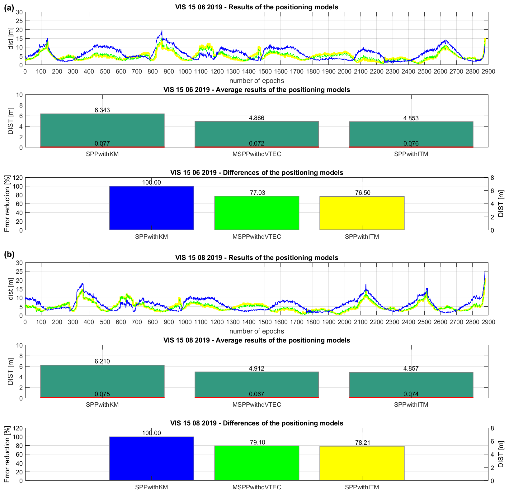
Figure 1 Set of the results of the positioning models: (a) VIS 15 June 2019 and (b) VIS 15 August 2019.

3 Numerical experiment and discussion

In this section, the explanation of the research concept will be done. Next, the appropriate numerical experiment in view of graphics and numeric settings will be presented. The parallel discussion about obtained results for appropriate interpretation will be made.

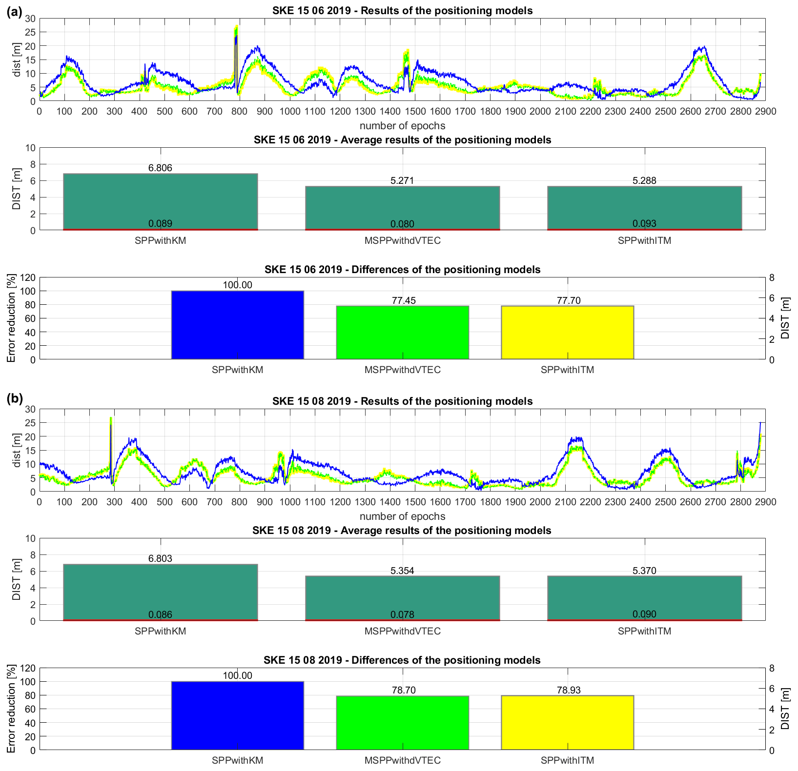
Figure 2 Set of the results of the positioning models: (a) SKE 15 June 2019 and (b) SKE 15 August 2019.

3.1 Research concept

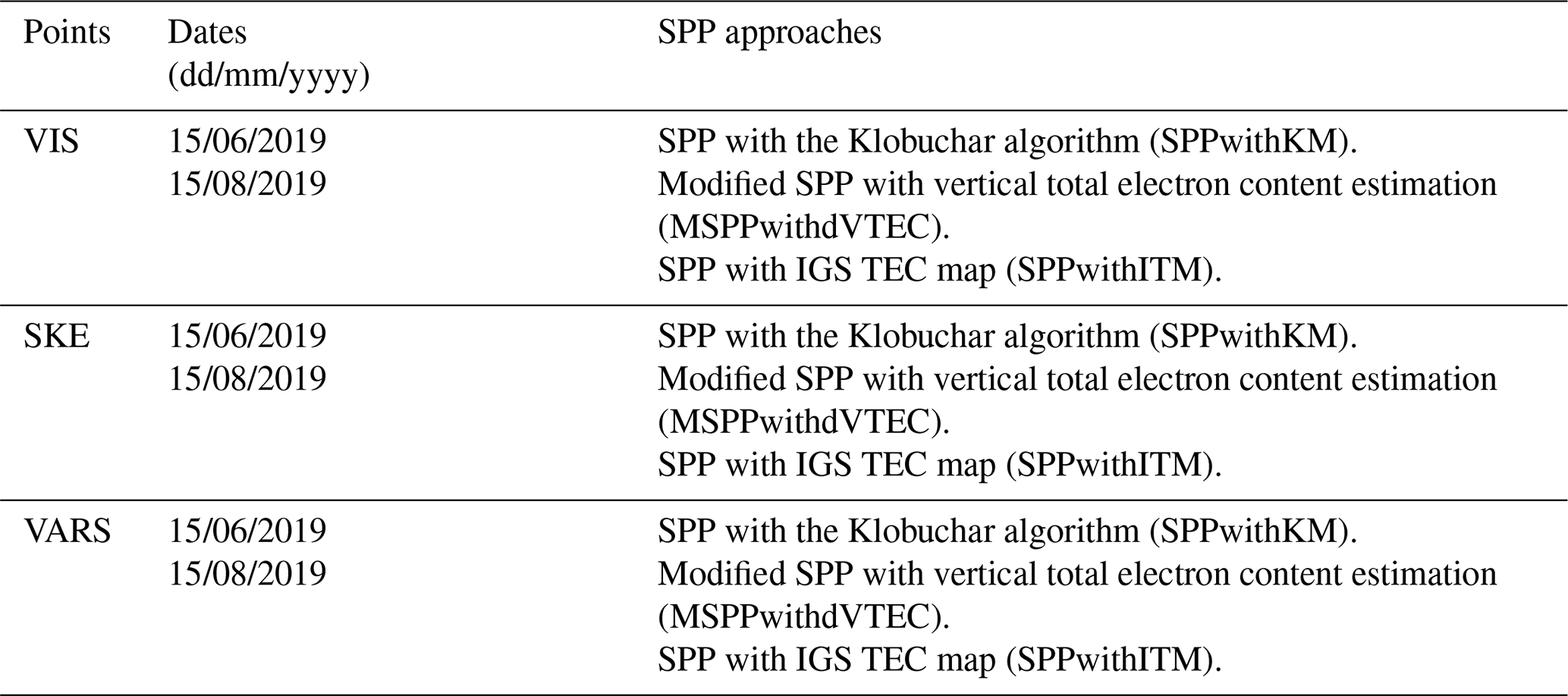
The numerical experiment is based on real single-frequency code pseudo-range observations from GPS, namely C1C code data on the L1 carrier frequency (1575.42 MHz). Continuing, three different EUREF (Regional Reference Frame Sub-Commission for Europe) Permanent GNSS Network stations have been chosen in Scandinavia: two stations in Sweden – Visby (VIS) and Skellefteå (SKE) – and one in Norway – Vardø (VARS). The observational files and initial coordinates of receivers were gained from the BKG (Bundesamt für Kartographie und Geodäsie) GNSS Data Center. The parameters of precise satellite orbits (SP3 file), broadcast ephemeris data and atmospheric data were obtained by means of CDDIS (Crustal Dynamics Data Information System) – in fact, IONEX only in view of atmospheric data, as a source of IGS TEC map. The coordinates of points were treated as the true coordinates in the practical part of the experiment. The reference coordinates are presented in Table 1.

Table 1 Actual coordinates of points.

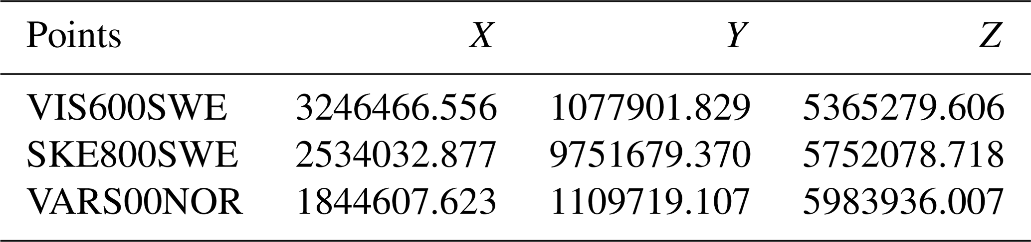
In the models, the actual coordinates have been converted to the antenna phase centre to make a comparative analysis with the SPP results, where measurements were executed to the antenna phase centre.

Three different localizations allow checking how the modified SPP model works on different geodetic latitudes because of ionosphere activity changes, so its quality in the GPS code domain can be widely stated.

The research concept focuses on measurement on two different days in the cited locations. Therefore, three stations of the EUREF Permanent GNSS Network were employed for comparative analysis based on data from two parallel days.

Table 2 Experiment concept.

To execute the numerical experiment of the research, the MATLAB environment from MathWorks was used. The “PostCalc” software developed by Dawid Kwaśniak was utilized as the base MATLAB programme. Next, the complementary changes were done by the authors of paper because of the numerical experiment requirement.

3.2 Discussion of the experiment results

Figures 1–3 present the distribution of dist values during the observational day (results of the positioning models) and their average value (DIST) with appropriate mean errors in the middle (average results of the positioning models). In turn, the bottom parts show the error reduction of the models (differences of the positioning models). The upper part of Fig. 1a demonstrates the solutions for Visby station on 15 June 2019. The dist results are significantly improved for MSPPwithdVTEC, referring to the SPPwithKM which is confirmed by the average value of DIST equal to 4.886 m. There is not a major difference of DIST between MSPPwithdVTEC and SPPwithITM (0.033 m). Therefore, the mean error of DIST (0.072 m) affirms the precision of the modified solution. Studying the bottom division of Fig. 1a, SPPwithKM was assumed as a reference one (100 %) in the calculation of the percent values of error reduction based on DIST. The results are satisfying because of error reduction on the level of 22.97 % in the MSPPwithdVTEC case and the close discrepancy with the error reduction of the SPPwithITM (0.53 %). The second day of using Visby station is 15 August 2019. In the middle of Fig. 1b, DIST is beneficial for the MSPPwithdVTEC (4.912 m) compared to the reference model, which leads to defining the tendency of improved accuracy in the SPP. Again, the difference in the average solutions of DIST between MSPPwithdVTEC and SPPwithITM is insignificant (0.055 m) according to code observations accuracy level. Thus, the accuracy of the estimation method is comparable with the IGS TEC map. Focusing on the average explanation of the DIST mean errors among the MSPPwithdVTEC (0.067 m) and the SPPwithITM (0.074 m), these approaches do not distinctly vary, which indicates that the proposed SPP model works well. At the bottom of Fig. 1b, the error reduction of the MSPPwithdVTEC is 20.90 % and is at a similar level with the SPPwithITM (21.79 %). The SPPwithKM proved to be the lowest accuracy method. Probably, the ionospheric corrections obtained by the coefficients from the navigation message cannot reflect the changes that take place in the ionosphere with the higher temporal accuracy. Briefly, in the first studied point, the MSPPwithdVTEC can be judged as the precise SPP model.

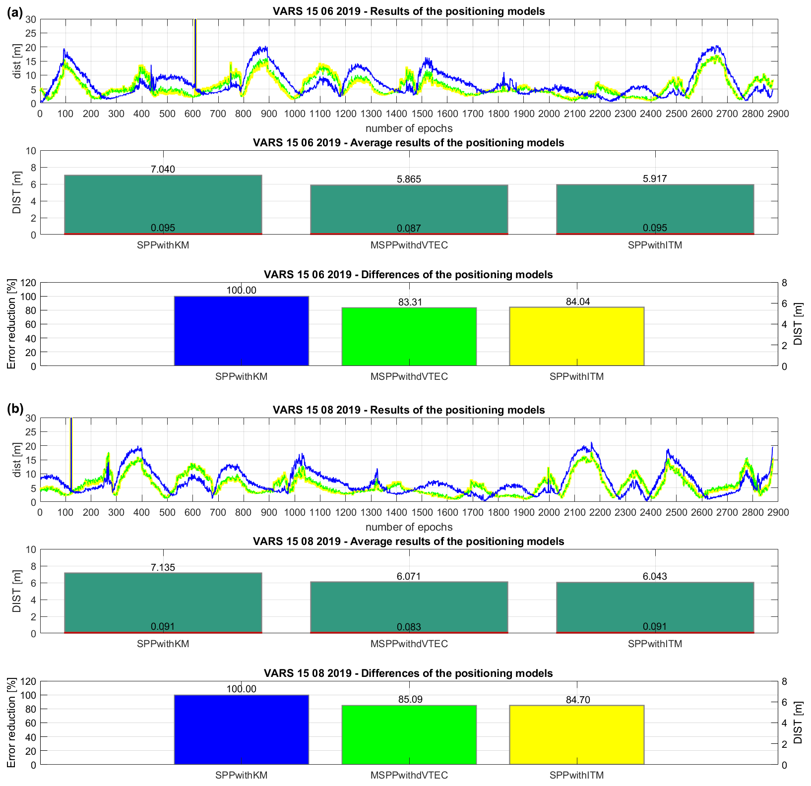
Figure 3 Set of the results of the positioning models: (a) VARS 15 June 2019 and (b) VARS 15 August 2019.

Following the experiment report, the next examined subject is SKE on 15 June 2019. Looking at Fig. 2a, the top part presents the dist distribution of the MSPPwithdVTEC solutions close to the SPPwithITM. The average description of DIST validates this declaration, where the difference between these two approaches is 0.017 m, in favour of the MSPPwithdVTEC. In turn, according to the base model, the MSPPwithdVTEC delivers solutions with highly increased accuracy, which is the most important. Despite such accuracy, the DIST precision of the MSPPwithdVTEC (0.080 m) is improved and is at a similar level to SPPwithITM (0.093 m), which confirms the consistency of the methods. Explaining the bottom part of Fig. 2a, the error reduction of the MSPPwithdVTEC is at the beneficial level of 22.55 %, which is again close to the reduction obtained by the SPPwithITM (22.30 %). Therefore, this method can be evaluated as the approach of a similar class compared to the case with IGS TEC map. The second day of tests is 15 August 2019. Based on dist at the top of Fig. 2b, it is noticeable that the MSPPwithdVTEC results are at a relatively similar level to the SPPwithITM. Looking at the middle part of Fig. 2b, the increased accuracy in MSPPwithdVTEC is verified by the DIST solution equal to 5.354 m, referring to the initial SPPwithKM. The mean error of DIST gives an acceptable value using the MSPPwithdVTEC at a comparable magnitude with the other models. Considering the bottom part of Fig. 2b, the error reduction amounts to 21.30 %, whereas the approach with the IGS TEC map achieves an equivalent value of 21.07 %. In sum, the MSPPwithdVTEC can be assessed on the next EUREF location as the valuable SPP approach by use of the new method of the ionospheric refraction estimation, without the need for external products, e.g. atmospheric factors or GIMs.

The last studied point is VARS00NOR. The first examined day is 15 June 2019. The middle part of Fig. 3a demonstrates that the DIST difference of the two approaches: the SPPwithITM and MSPPwithdVTEC difference is 0.052 m; therefore, the improved accuracy is at a similar level, referring to the SPPwithKM average observations. The precision of DIST confirms the reliability of the MSPPwithdVTEC, where the mean error is equal to 0.087 m with an insignificant discrepancy (0.008 m) compared to the SPPwithITM. The bottom part of Fig. 3a shows a decrease in the percent value of the error reduction. The error reduction of the MSPPwithdVTEC is at the level of 16.69 %; thus, the improvement of accuracy is verified. Again, the difference of error reduction among MSPPwithdVTEC and SPPwithITM is on a parallel level (0.73 %), which confirms the method credibility. The second tested day, and therefore the last one, is 15 August 2019. The DIST elaboration in Fig. 3b presents the low differences between the two principal approaches on the level of 0.028 m. Studying the bottom division of Fig. 3b, the MSPPwithdVTEC achieves a positive level of error reduction of 14.91 %, relating to the SPPwithKM. In addition, the top parts of Fig. 3a and b present the distribution of the MSPPwithdVTEC dist results as close in value to the SPPwithITM with increased accuracy to the SPPwithKM. This finding is also valid for other examined cases. Thus, the proposed model can be identified as stable and accurate. The error reduction is at a satisfactory level.

Focusing on the mean errors of the final solution in the NEU system, we will consider the average precision of the differences of the components ΔN, ΔE and ΔU, referring to the daily result. The difference indicates the discrepancy between the actual station's coordinates and the received position from the SPP methods. For this purpose, Eq. (26) was used to determine the mean values of ΔN, ΔE and ΔU errors which are summarized in Table 3.

Table 3 Average errors of the difference in the positions using the NEU system.

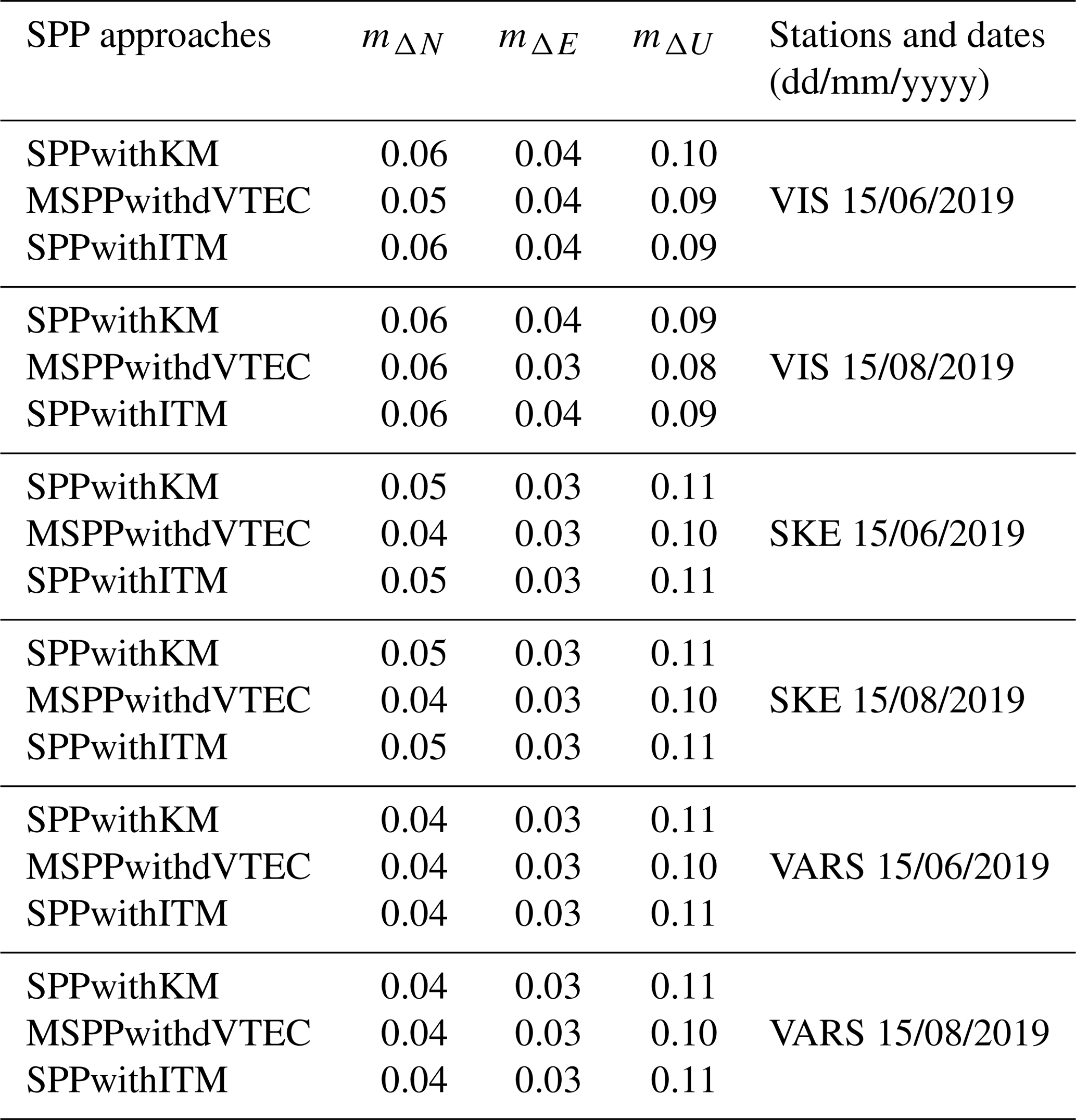
The error quantities of the difference in the positions were achieved for the MSPPwithdVTEC and SPPwithITM on a close level. Separating the horizontal and the vertical components of the position, the MSPPwithdVTEC is characterized by comparable precision to SPPwithKM in the north and east directions; therefore, the additional estimated parameter in the code equation does not change the SPP model enough to reduce its quality. The case is repeated in the context of the vertical component U. The MSPPwithdVTEC is profitable and achieves the similar values of the mean errors to SPPwithITM. In general, the values are close to each other and the differences are not as clear in the context of the code data use. Therefore, the quantities of average errors demonstrate that MSPPwithdVTEC is the approach of the closest precision to the SPPwithITM, specified as a high-quality product, which is the most important from the authors' point of view.

4 Conclusions and future perspectives

The main idea of this paper was to introduce the new method to estimate the ionospheric delay in the SPP without using the external data. Moreover, in the case of comparative analysis, two common approaches in SPP were employed: SPP with the Klobuchar algorithm and SPP with IGS TEC map. The first one was treated as a reference one. The SPP model with IGS TEC map was utilized to authenticate the proposed model in view of IGS TEC map use – defined as a high-quality product. The explanation of mathematical models and appropriate accuracy analysis criteria were done. Next, the numerical experiment using real code data from three different GNSS stations with discussion to interpret the obtained results was conducted. Referring to achieved solutions, the proposed approach can be defined as a simple and independent way to improve SPP. Moreover, the MSPPwithdVTEC can be employed in the procedure of determining the approximate position for the need of the single-epoch precise positioning.

Based on the mean distance of the solution from the true position, the MSPPwithdVTEC achieved improved GPS position in comparison to the basic SPPwithKM in each tested station. Moreover, the MSPPwithdVTEC acquires a similar level of error reduction to the SPPwithITM, which is the most satisfying in view of method authentication.

Finally, the results of the MSPPwithdVTEC confirm the potential use of the mathematical model in the SPP. The strategy should be developed in the future through the verification of model stability in the other stations since ionosphere changes are highly dependent on localization. Therefore, the proposed method of SPP can be recognized as a good forecast to become independent of external products delivering information about the ionospheric delay.