Experiments on magnetic interference for a portable airborne magnetometry system using a hybrid unmanned aerial vehicle (UAV)

Using unmanned aerial vehicles (UAVs) for airborne magnetometry offers not only improved access and rapid sampling but also reduced logistics costs. More importantly, the UAV-borne aeromagnetometry can be performed at low altitudes, which makes it possible to resolve fine features otherwise only evident in ground surveys. Developing such a UAV-borne aeromagnetometry system is challenging owing to strong magnetic interference introduced by onboard electric and electronic components. An experiment concerning the static magnetic interference of the UAV was conducted to assess the severity of the interference of a hybrid vertical take-off and landing (VTOL) UAV. The results of the static experiment show that the wing area is highly magnetic due to the proximity to servomotors and motors, whereas the area along the longitudinal axis of the UAV has a relatively smaller magnetic signature. Assisted by the static experiment and aerodynamic simulations, we first proposed a front-mounting solution with two compact magnetometers. Subsequently, two dynamic experiments were conducted with the setup to assess the dynamic interference of the system. The results of the dynamic experiments reveal that the strongest source of in-flight magnetic interference is the current-carrying cables connecting the battery to the flight controller and that this effect is most influential during pitch maneuvers of the aircraft.

1 Introduction

Magnetic surveying has been extensively used in the search for mineral deposits, oil and gas reservoirs, and geothermal resources, as well as for a variety of other purposes, such as natural hazards assessment, basement structural studies, mapping subsurface archeology, and unexploded ordnance (UXO) (Nabighian et al., 2005; Hinze et al., 2013; Kruse, 2013; Haldar, 2018; Turner et al., 2015). In general, magnetic measurements can give insight into the physical, chemical, and even biological processes that have affected the iron phases within.

Airborne magnetometry (aeromagnetometry) is an inexpensive, efficient, and effective regional reconnaissance tool (Reeves, 2005). The method offers improved accessibility to areas previously restricted to terrestrial surveys, such as remote areas, offshore areas, and thickly vegetated regions, as well as a rapid sampling of the local geomagnetic field compared to its ground or space counterpart (Council, 1995; Haldar, 2018).

Conventionally, aeromagnetic surveys are often conducted using fixed-wing aircraft with sensors mounted on both wings (horizontal sensor configuration) or a tail-stinger behind the aircraft. Thanks to decades of development in noise-reduction techniques coupled with new advances in sensor technologies, such modern aeromagnetic surveys can achieve a sensitivity of 0.1 nanotesla (nT) (Eppelbaum, 2015; Turner et al., 2015). Geophysicists have realized that aeromagnetometry using lightweight and compact platforms such as unmanned aerial vehicles (UAVs) can even further reduce surveying costs (Eppelbaum and Mishne, 2011; Tuck et al., 2018; Mu et al., 2020). More importantly, UAV-borne magnetometry systems are capable of flying with low terrain clearances, thereby improving detectability significantly (Eppelbaum and Mishne, 2011).

In the recent decade, the feasibility and effectiveness of lightweight UAV-borne magnetometry systems have been demonstrated by various geophysical applications, from identifying various rock types and structures in the subsurface and delineating ore deposits to locating synthetic ferrous objects, such as UXO (Perry et al., 2002; Cunningham, 2016; Malehmir et al., 2017; Parvar et al., 2017; Kolster and Døssing, 2021). However, developing a low-noise UAV-borne magnetometry system is challenging given the compact size of a UAV platform; i.e., magnetometers easily fall in the vicinity of sources of magnetic interference from the platform, such as motors, electric-powered devices, and even current-carrying cables (Forrester, 2011; Sterligov and Cherkasov, 2016; Hansen, 2018; Tuck et al., 2018; Tuck, 2019). As a result, UAV-borne magnetometry systems are often suspended in a magnetometer bird (housing magnetometers, global navigation satellite system (GNSS) antenna, and a data logger) a few meters below the airframe to minimize the interference from the platform (Malehmir et al., 2017; Parvar et al., 2017; Parshin et al., 2018; Sterligov et al., 2018; Nikulin and de Smet, 2019). This configuration is only slightly prone to the magnetic interference from the platform, but this is at the cost of efficiency and positioning accuracy (Tuck et al., 2018). Alternatively, magnetometers may be mounted directly on a boom attached to the UAV airframe (Samson et al., 2010) or on the wing tips of the platform (Wood et al., 2016).

To facilitate high-resolution and efficient UAV-borne magnetometry, we intended to develop a lightweight (less than 10 kg), efficient (more than 70 km per charge), and flexible (vertical take-off and landing) UAV-borne magnetometry system, capable of conducting magnetic surveys in various terrains. To meet the requirements, we chose a hybrid fixed-wing UAV platform capable of taking off and landing vertically. To determine the optimal placement of the magnetometers, a good understanding of the magnetic interference of the platform is necessary at the early stage of the development. For example, Forrester (2011) and Sterligov and Cherkasov (2016) successfully mapped magnetic signatures of the UAVs and also managed to locate sources of interference. However, they neglected to address the complex interplay between active and passive components (Tuck et al., 2018). Therefore, Tuck et al. (2018) proposed a systematic method to investigate magnetic interference of UAVs and demonstrated their method on a 25 kg fixed-wing UAV. Instead of investigating every possible source from the platform, we will present a static and two dynamic experiments to investigate both the static and dynamic magnetic interference and their interplay from the platform in operation.

2 Platform – a hybrid VTOL UAV

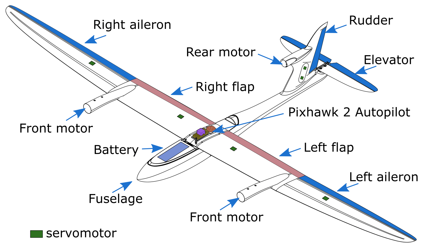
The UAV for the airborne magnetometry system is a beta prototype version of a hybrid vertical take-off and landing (VTOL) UAV from Kapetair. The UAV is capable of taking off and landing vertically without a runway, so it can be deployed in various terrains. It is also capable of flying in both multi-rotor mode and fixed-wing mode. The UAV has three position-adjustable motors. The two front motors are used for multi-rotor mode. The third (tail) motor is used for take-off and landing and provide thrust during the fixed-wing (cruise) mode; i.e., the front motors stay inactive during the cruise mode, and only the rear motor remains active. The fuselage of the UAV houses various hardware components, including a flight controller (FC), several electronic speed controllers (ESC), an inertial measurement unit (IMU), a global navigation satellite system (GNSS) module, a radio-frequency (RF) module, a data-logger for magnetometry, and a few cables connecting those components. A 22 000 mAh Li-Po battery is also placed in the front of the fuselage. The technical specifications of the platform are listed in Table 1.

Table 1 Specifications of Kapetair VTOL UAV.

Figure 1 Schematic view of the layout of the UAV.

Source of magnetic interference

For a lightweight UAV platform such as the Kapetair VTOL UAV, brushless direct-current (BLDC) motors are often used due to their better speed control, higher efficiency, and compact design (Juliani et al., 2008). BLDC motors are comprised of permanent magnets and solenoids, which can generate a strong magnetic signature. The BLDC motors are driven to revolve by sending tuned pulses of current to the solenoids, which means constant electrical switching, probably causing discontinuous magnetic interference. Tuck et al. (2018) observed magnetic interference due to the current-carrying cables connecting the ESC to the batteries. According to Ampere's law, the magnetic field is proportional to the electric current. Therefore, the magnetic interference varies with the current in the cables. In addition, the airframe of the UAV is composed of carbon fiber, which is non-magnetic but conductive, akin to graphite (Chung, 2010). As a result, eddy currents (Stoll, 1974) may play a role in magnetic interference during flight. Finally, the onboard avionics system that is comprised of several electronic components (such as the FC module, the IMU module, the GNSS module) may generate complex electromagnetic interference. A rule of thumb is, therefore, always to place magnetometers as far away as possible from the UAV components that are magnetic.

3 UAV magnetic signature mapping – static experiment

An airborne magnetometry system using a compact UAV platform is affected by the UAV's magnetic signature (Tuck et al., 2018). Mapping the magnetic signature of a UAV is useful to identify magnetic highs and lows of the UAV and pinpoint favorable regions less susceptible to the UAV's magnetic interference. Because the magnetic signature varies from platform to platform, it is imperative to map a specific platform's magnetic signature.

3.1 Method

The magnetic signature mapping of the Kapetair UAV was carried out at the Brorfelde geomagnetic observatory in Denmark. A customized 2300 × 958 × 700 mm wooden frame was built for the experiment (Fig. 2). Since the magnetic signature of a UAV can change significantly over a few centimeters, it is beneficial to have the magnetic signature on a fine grid with cells of 10 × 10 cm (Sterligov and Cherkasov, 2016). However, such an approach is time-consuming if carried out manually. We adopted a slowly revolving DC motor to pull a slider holding a high-precision potassium scalar magnetometer (GSMP-35U from GEM Systems). The sampling rate of the magnetometer was set to 10 Hz and the speed of the slider was 2 cm s⁻¹ on average. The DC motor, a laptop for data logging, and two power supplies were placed in another room away from the measurement. Due to the limited space in the observatory, only one wing and the mainframe were measured at once (Fig. 2). The UAV remained off during the magnetic signature measurement.

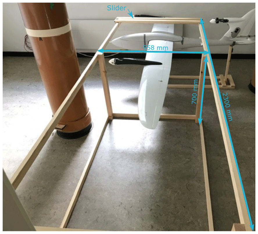
Figure 2 Demonstration of the magnetic signature measurement of the port wing. The length and the width of the slider are 1000 and 150 mm, respectively.

3.2 Magnetic signature

With the help of the semiautomatic magnetic measurement, we collected more than 70 000 magnetic observations of the magnetic signatures of the starboard wing, the port wing, and the area along the longitudinal axis of the UAV, together with their respective background field. The background fields and the magnetic signatures experienced diurnal corrections. After the diurnal corrections and background removal, the corrected magnetic signatures were gridded on a planar surface with a 2.5 cm grid interval shown in Fig. 3. As seen in Fig. 3, the magnetic signature of the wing area has a high amplitude (up to 600 nT) and peaks over the servomotors and the motors. The servomotors make a major contribution to the overall magnetic signature of the UAV, their magnetic signatures also decrease rapidly with distance toward the main fuselage of the platform. For a high-resolution aeromagnetic system, the standard of commercial aeromagnetic practice that only allows a noise envelope of 0.1 nT (Reeves, 2005) requires the magnetometers to be mounted in places with the least magnetic signature. Due to the high magnetic signatures of the servomotors, we replaced the originally highly magnetic servomotors with BLDC servomotors with a smaller magnetic signature (see Fig. 4b).

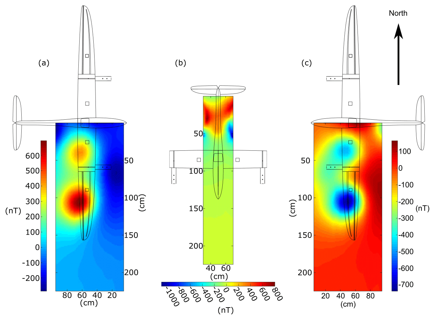
Figure 3 The diurnal-corrected and background-subtracted magnetic signature: (a) the starboard wing, (b) the area along the longitudinal axis of the UAV, and (c) the port wing.

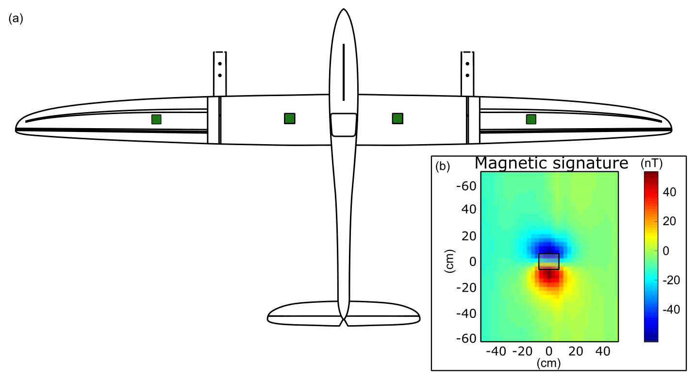
Figure 4 Locations of the replaced servomotors and the magnetic signature of the new BLDC servomotor: (a) the locations of the replaced servomotors, indicated by green squares, and (b) the magnetic signature of the new low-magnetic servomotor. The small black square in the middle indicates where the servomotor was located, and the servomotor was off during the measurement. The measurement was conducted on a planar 10 cm above the servomotor.

According to the map of the magnetic signature (Fig. 3), the wing tips and the nose tip are magnetically low-amplitude zones. Mounting two magnetic sensors at the tip of the wings renders it possible to measure the horizontal gradient, which is useful for both data-processing and interpretation purposes. However, the wings are deliberately flexible to adapt to dynamic airflow in flight; i.e., the high-frequency vertical displacement due to the flexibility (readily up to 120 mm) during flight may introduce unpredictable noise (Tuck et al., 2018). Moreover, aerodynamically, the wing tips are sensitive to the disturbance caused by geometric changes; i.e., mounting magnetometers onto the wings' exterior may lead to wing stall and even a crash.

4 A front-boom setup

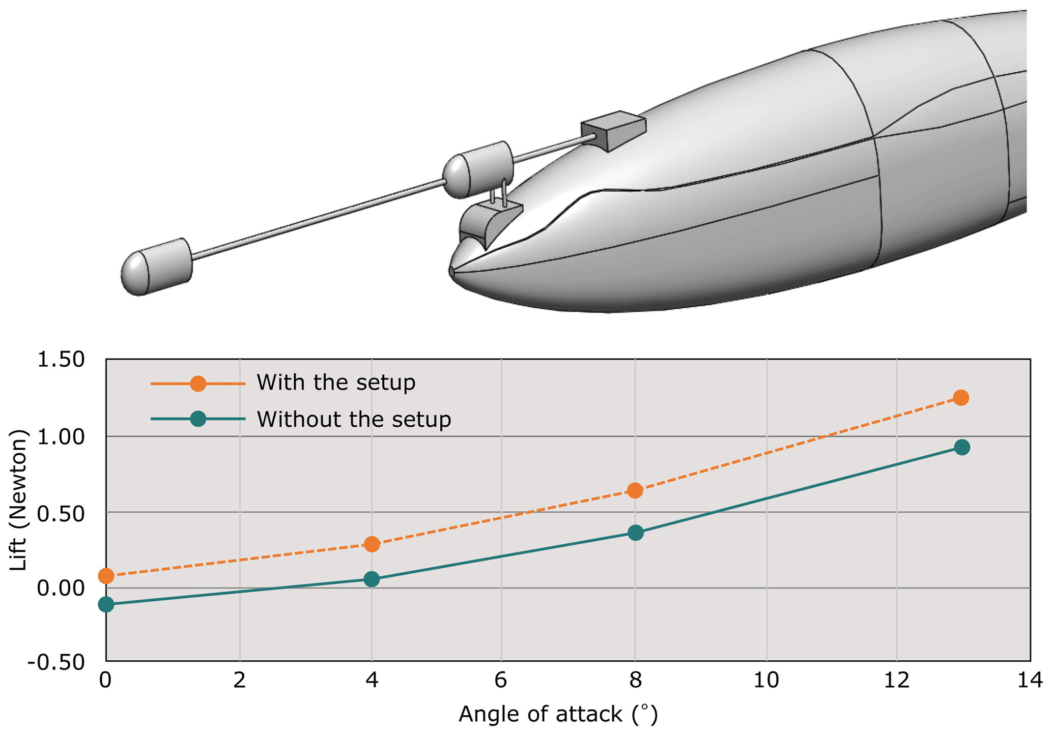
Mounting magnetometers on the nose tip does not provide the typical horizontal gradient but provides an aerodynamically stable solution (see Fig. 5). This configuration will theoretically not cause any aerodynamic instability because the geometric modification to the nose area should cause only small aerodynamic forces. We carried out a computational fluid dynamics (CFD) simulation on the fuselage to investigate the aerodynamic stability of the nose setup. The plot (Fig. 5, lower panel) shows that the influence introduced by adding the mount on the nose is negligibly small, with the maximum magnitude of lift forces being around 1 N (compared to the total lift force of the UAV during leveled flight of around 60 N, as it should balance a mass of 6 kg). In principle, the center of gravity (CG) can be fixed by adjusting the battery position and some changes in the moment of inertia can be easily handled by the flight controller. A flight test with this setup showed stable behavior of the UAV, confirming that the change in the moment of inertia is within the capabilities of the flight controller. Increasing the boom length does not cause significant aerodynamic forces as long as the rod is kept at small angles in relation to the airflow during flight.

Figure 5 The nose-mounting solution and its aerodynamic forces.

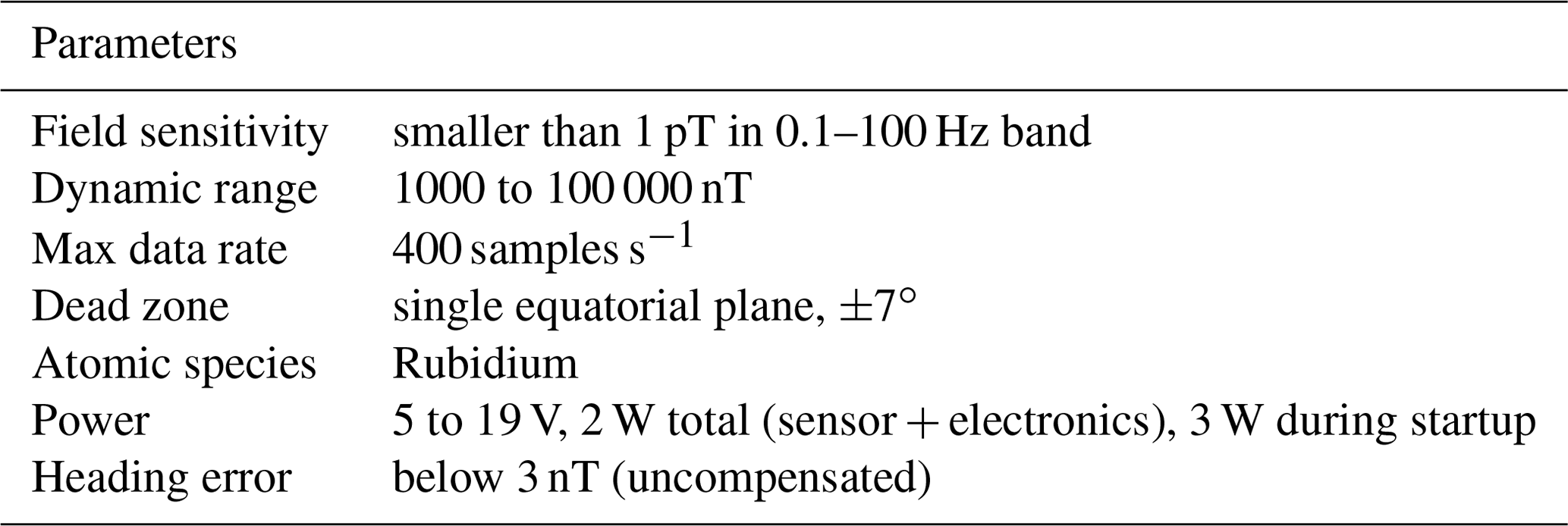
Based on the results of the static experiment and the aerodynamic analysis, some changes were made to the initial setup (Fig. 5), resulting in the two magnetometers on the boom now being placed further away from the aircraft (Fig. 6) to further reduce the magnetic noise from the UAV. Meanwhile, the two-magnetometer setup provides a solution that eases the filtering of the magnetic noise (Chen et al., 2018; Mu et al., 2020). The two compact magnetometers are manufactured by QuSpin, abbreviated as QTFM. The QTFM is a compact, low-power, and high-sensitivity scalar magnetometer that is capable of sampling the geomagnetic field over 200 times per second (Table 2). The primary magnetometer (front magnetometer) is responsible for observing the geomagnetic field, whereas the secondary sensor placed closer to the nose tip is used to monitor the in-flight noise from the platform. The distance d is used to indicate the distance between the primary and secondary magnetometer, whereas L is for the distance between the secondary magnetometer and the mounting point on the UAV (see Fig. 6).

Figure 6 Side view of the final front-boom-mounted setup.

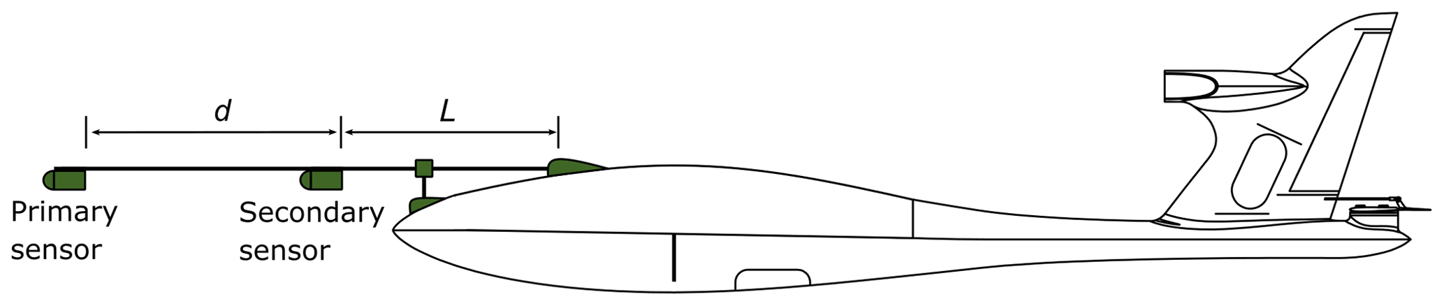
Table 2 Specifications of QuSpin total field magnetometers (QTFM).

5 UAV in-flight magnetic signature – dynamic experiment

To understand the real dynamic noise of the UAV in operation, we flew two dynamic experiments in Støvring, Denmark (Fig. 7). The test site is covered with up to 12 km of unmetamorphosed sediments lodged over the crystalline basement, and the surface of the region consists mainly of unconsolidated Quaternary glacial and interglacial deposits (Håkansson and Surlyk, 1997). Normally, sediments are considered non-magnetic, which is the basis for many applications of aeromagnetic surveys (Reeves, 2005). As a result, the local magnetic field is insignificant, which renders the data collected during the dynamic experiment a direct reflection of the dynamic noise from the platform.

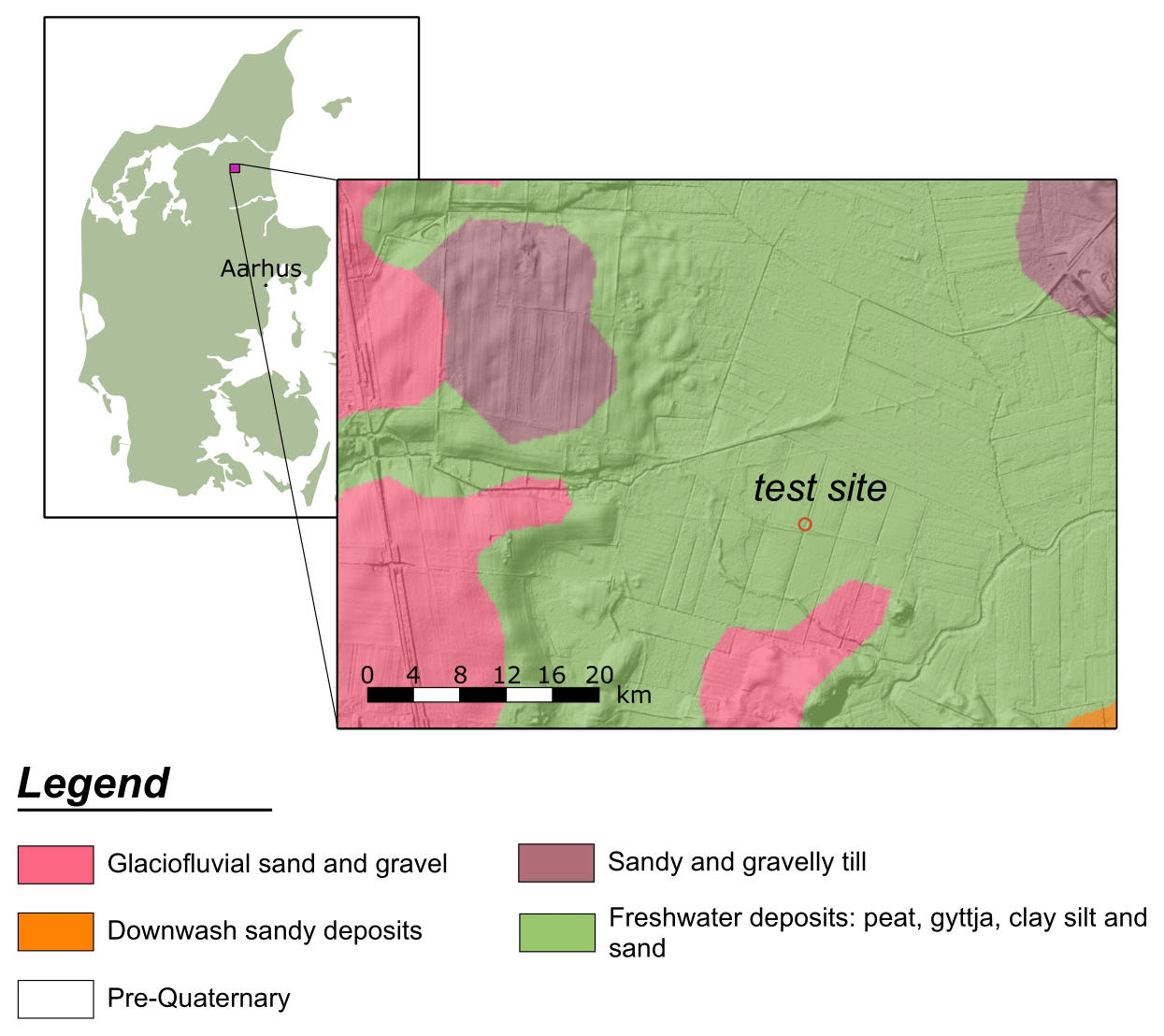
Figure 7 Location and surface geology of the test site according to Surface Geology Map of Denmark 1 : 200 000. The surface geology map of Denmark at a 1 : 20 000 scale is credited to Pedersen et al. (2011), and the map of Denmark is credited to https://MapSVG.com (last access: 25 January 2021).

5.1 Method

Dynamic effects that originate from revolving solenoids, permanent magnets, eddy currents, or loose current-carrying cables can be divided into discontinuous and continuous noise. The discontinuous noise appears as isolated spikes or a set of closely spaced spikes on an aeromagnetic profile, which is typically associated with the pilot's actions such as radio transmissions and switching direct current, along with lightning strikes or cultural sources (e.g., trains, power lines) (Reeves, 2005; Eppelbaum, 2011, 2015). The continuous noise comes from the motions of the aircraft, such as the oscillation of wings due to turbulent weather. The empirical real-time fourth difference is widely used for monitoring the in-flight discontinuous noise in aeromagnetometry (Reeves, 2005). Complying with the widely accepted industry standard, the fourth difference should lie between ±0.05 nT (or 0.1 nT peak to peak) (Coyle et al., 2014; Cunningham, 2016). The fourth difference for an airborne magnetic survey can be calculated as follows:

$$\begin{array}{}\text{(1)}& \mathrm{\text{fourth difference}}={\displaystyle \frac{T_{-\mathrm{2}}-\mathrm{4}{T}_{-\mathrm{1}}+\mathrm{6}{T}_{\mathrm{0}}-\mathrm{4}{T}_{+\mathrm{1}}+T_{+\mathrm{2}}}{\mathrm{16}}},\end{array}$$

where T₋₂, T₋₁, T₊₁, and T₊₂ are five consecutive readings centered on the current reading T₀.

5.2 The first dynamic experiment – multi-rotor mode

The first dynamic experiment was flown on 13 January 2020. The front-mounting boom (Fig. 6) was configured as d=20 cm and L=20 cm. The sampling rate of the QTFMs was set to 200 Hz. The UAV was switched on with all required components in position (such as the magnetometers, the power supply for the system). At first, the UAV was placed on the ground while the pilot was conducting the last-minute check. During this time, the magnetometers could observe dynamic interference from the UAV irrelevant to motions. In this pre-take-off phase (hereafter called “standby phase”) and with only a few UAV components being active, the power consumption of the UAV should be low, and the current in the cables connecting the battery with the flight controller should be low as well. As a result, the observed magnetic interference in the standby phase should mainly arise from the current-carrying cables in the front of the fuselage, permanent magnets of the actuators, and radio transmission (alongside dynamic and/or static cultural noise in the vicinity). Figure 8 shows residual magnetic intensity (RMI) with the International Geomagnetic Reference Field (IGRF) being removed from the raw magnetic measurements collected in the standby phase. As seen in Fig. 8, the plots show continuous superimposed effects of the magnetic interference from the UAV, cultural noise in the vicinity, and the magnetic field by the local geology (probably a constant offset). The RMI shown in the top panel in Fig. 8 is oscillating around 2.8 nT with mean variations of less than 0.5 nT, probably due to radio transmission and cultural noise. The average difference between the data from the primary and secondary magnetometer in this configuration is around 45 nT, even when the UAV is on standby. The fourth difference of the measurements from the primary magnetometer is spiky and lies within ±0.15 nT, significantly higher than the industry standard, whereas the fourth difference of the magnetic profile recorded by the secondary magnetometer (Fig. 8) is even bigger, up to ±1 nT. The difference in the fourth difference indicates that the interference mainly originated from the UAV rather than the surroundings because the secondary magnetometer is closer to the source of interference. The distance between the two magnetometers attenuates the interference, leading to the relatively smaller fourth difference of the data output by the primary magnetometer.

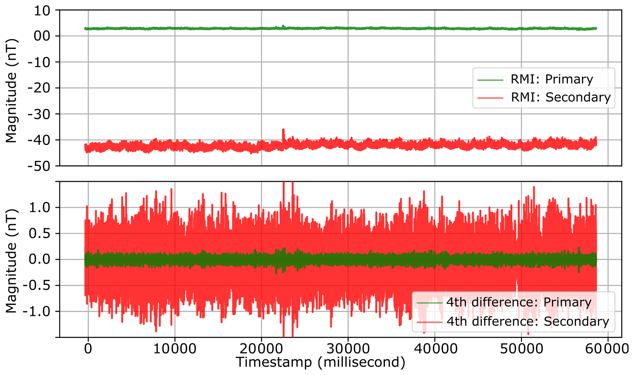
Figure 8 Data excerpt of RMI profiles recorded by the primary and secondary magnetometer and their respective fourth difference while the UAV was on standby on 13 January 2020 with d=20 cm and L=20 cm. The IGRF (50 560 nT) has been removed.

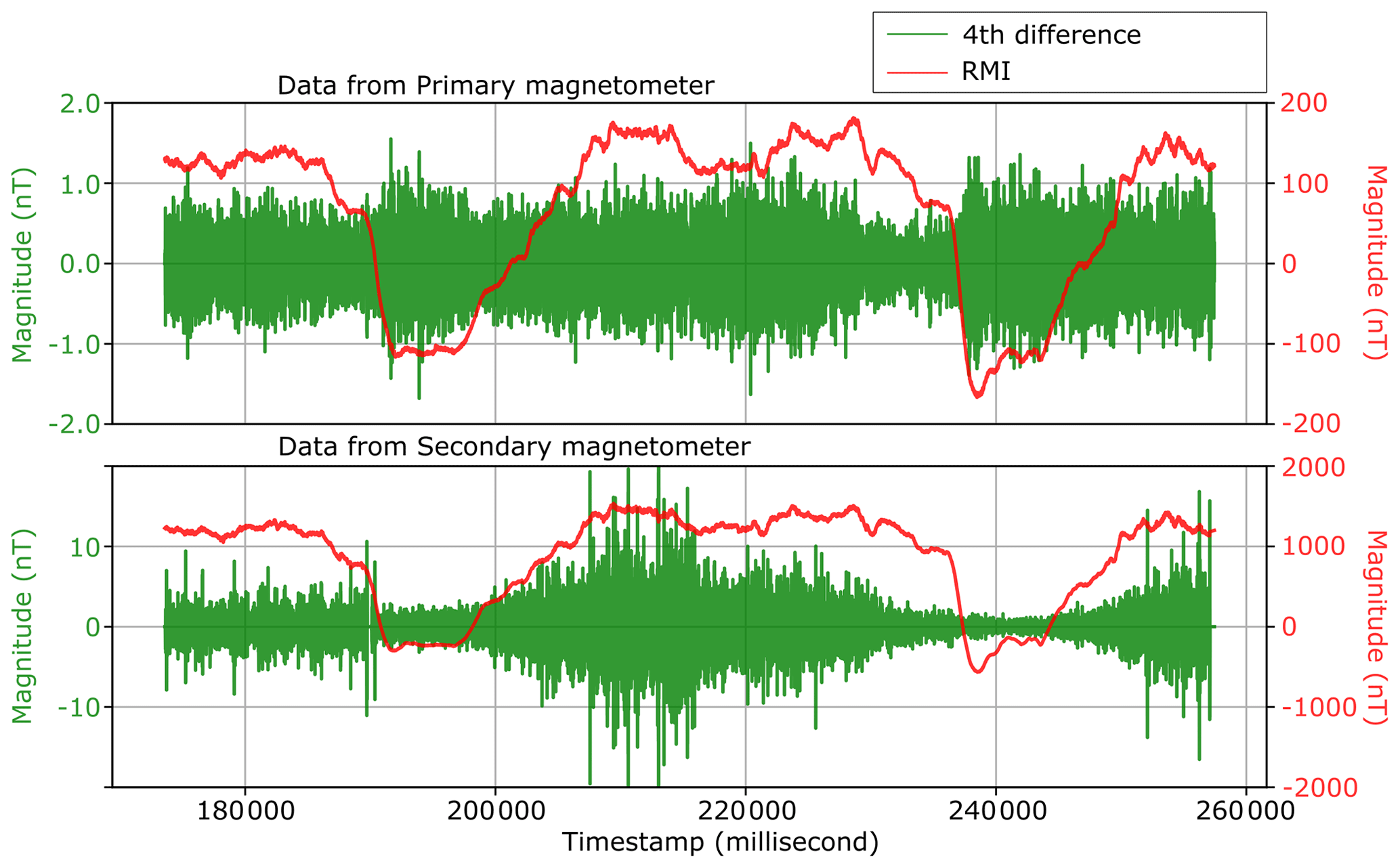
Figure 9 Data excerpt of RMI profiles recorded by the primary and secondary magnetometer and their respective fourth difference while the UAV was flown manually in the multi-rotor mode on 13 January 2020 with d=20 cm and L=20 cm. The IGRF (50 560 nT) has been removed.

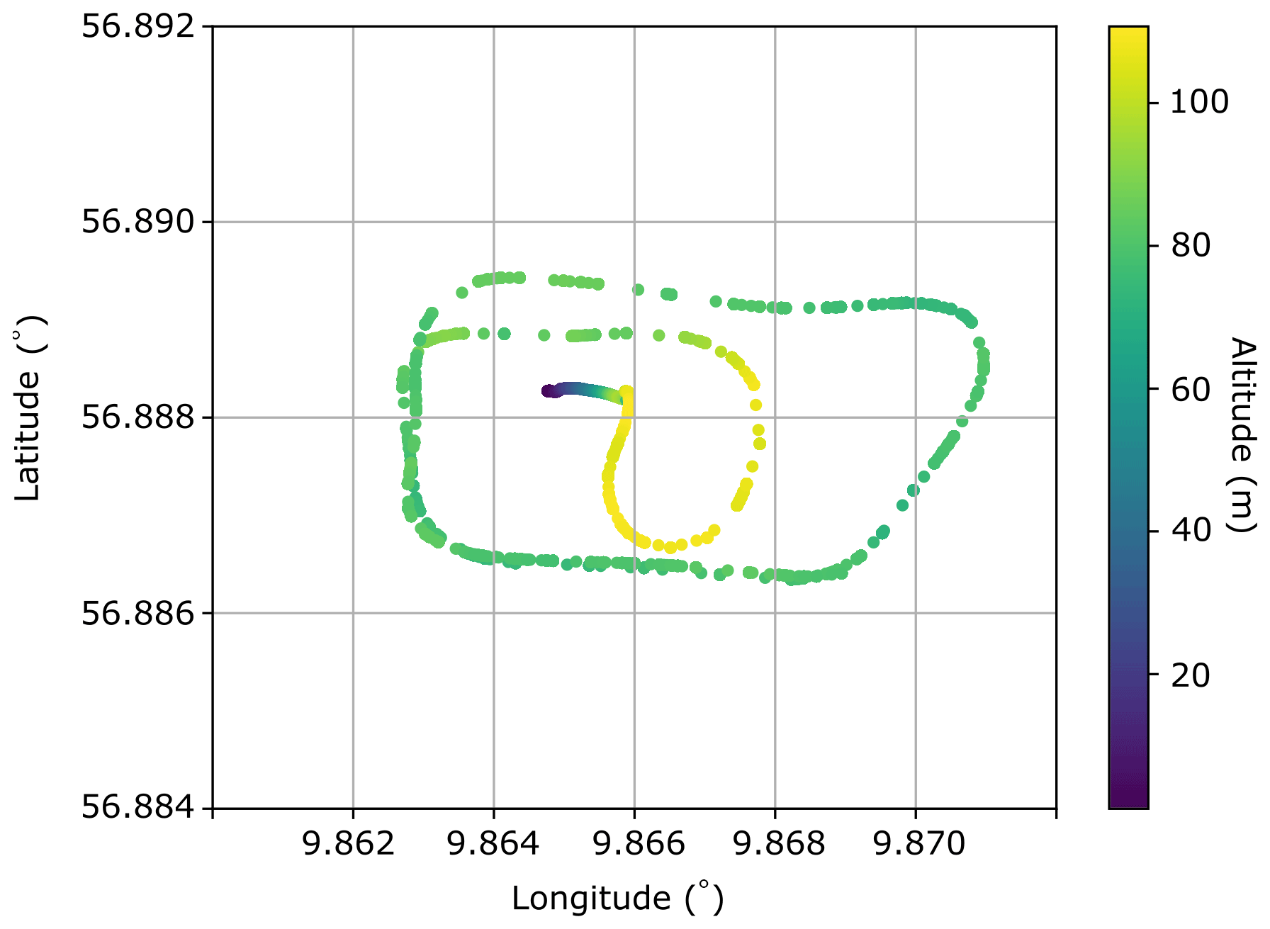
Following the standby phase, the UAV took off and was flown manually in the multi-rotor mode. Figures 9 and 10 show the in-flight RMI collected by the primary and secondary magnetometer and their respective fourth difference, together with its flight path. The two RMI profiles in Fig. 9 are almost identical in shape. The major difference lies in the magnitude. The RMI from the primary magnetometer is 10 times smaller than that from the secondary magnetometer. The in-flight fourth difference of the primary magnetic profile in Fig. 9 is spiky, with magnitudes up to ±1 nT, 20 times higher than the industry standard. The increase in the fourth difference is directly associated with the platform. It indicates that the observed signals from the two magnetic sensors are dominated by the noise from the platform. This noise could be due to the high output current flowing in the cables connecting the flight controller to the battery and the leakage of the alternating magnetic field from the BLDC motors in the multi-rotor mode. Nevertheless, in principle such strong noise can still be reduced by distancing the magnetic sensors even farther away from sources of magnetic interference.

5.3 The second dynamic experiment – fixed-wing mode

Because of the demonstrated strong interference from the UAV in the previous experiment, we increased the distance (L) between the secondary magnetometer and the mounting point to 30 cm to improve the signal-to-noise ratio. The distance (d) between the two magnetometers remained 20 cm. To reduce the dynamic noise observed in the first experiment and given that the aforementioned changes may lead to some instability, the UAV was also flown manually but in the fixed-wing mode for the second experiment. The sampling rate of the QTFMs was 200 Hz. The data collected in the standby phase and then during the fixed-wing flight are shown in Figs. 11, 12, 13, 14, and 15.

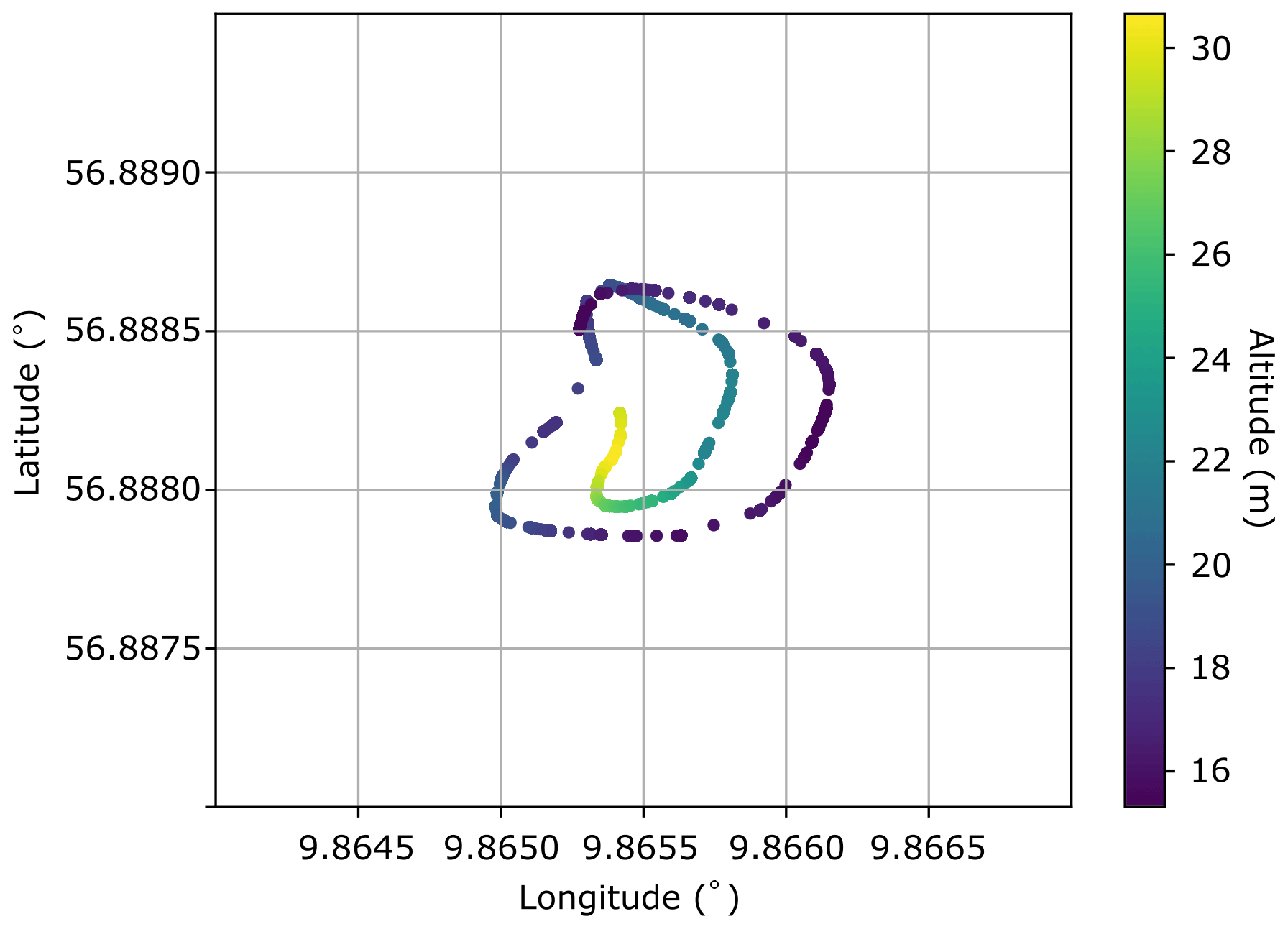
Figure 10 The production flight of the data excerpt shown in Fig. 9. The altitude indicates the in-flight height above mean sea level.

In comparison with the data gathered in the previous experiment, there is a noticeable increase in the magnitude of the RMI in Fig. 11, probably because of changes in the direct current flowing in the cables, the orientation of the cables, and even the actual distance between the magnetometers and the cables while the system in the field was being prepared. An extra metal GNSS antenna was deployed inside the fuselage to timestamp magnetic recordings during the first experiment, which was solely used at the beginning to synchronize the sensors, after which it was removed to reduce the magnetic interference. Nevertheless, the difference between the actual measurements from the two magnetometers was still surprisingly big, around 106 nT. The second experiment was conducted at the same test site as the first one, so the local geomagnetic field should remain roughly constant. Consequently, the big difference between the two magnetic profiles must be somehow introduced by the platform. Interestingly, the fourth difference of the measurements from the secondary magnetometer is slightly bigger than that of the data from the primary magnetometer within an envelope of ±0.2 nT. Since the fourth difference of the primary and secondary magnetic profiles is comparable in magnitude, it is difficult to say whether the noise originates mainly from the platform or cultural noise in the vicinity. It is clear that with the longer boom, the signal-to-noise ratio irrelevant to aircraft maneuvers is improved significantly, especially for the secondary magnetometer.

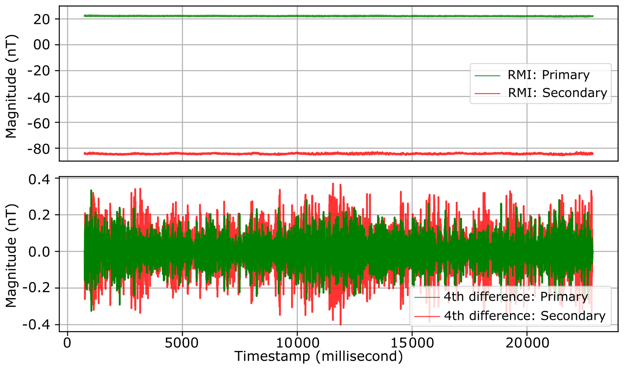
Figure 11 Data excerpt of RMI profiles recorded by the primary and secondary magnetometer and their respective fourth difference while the UAV was on standby with d=20 cm and L=30 cm on 5 March 2020. The IGRF (50 563 nT) has been removed.

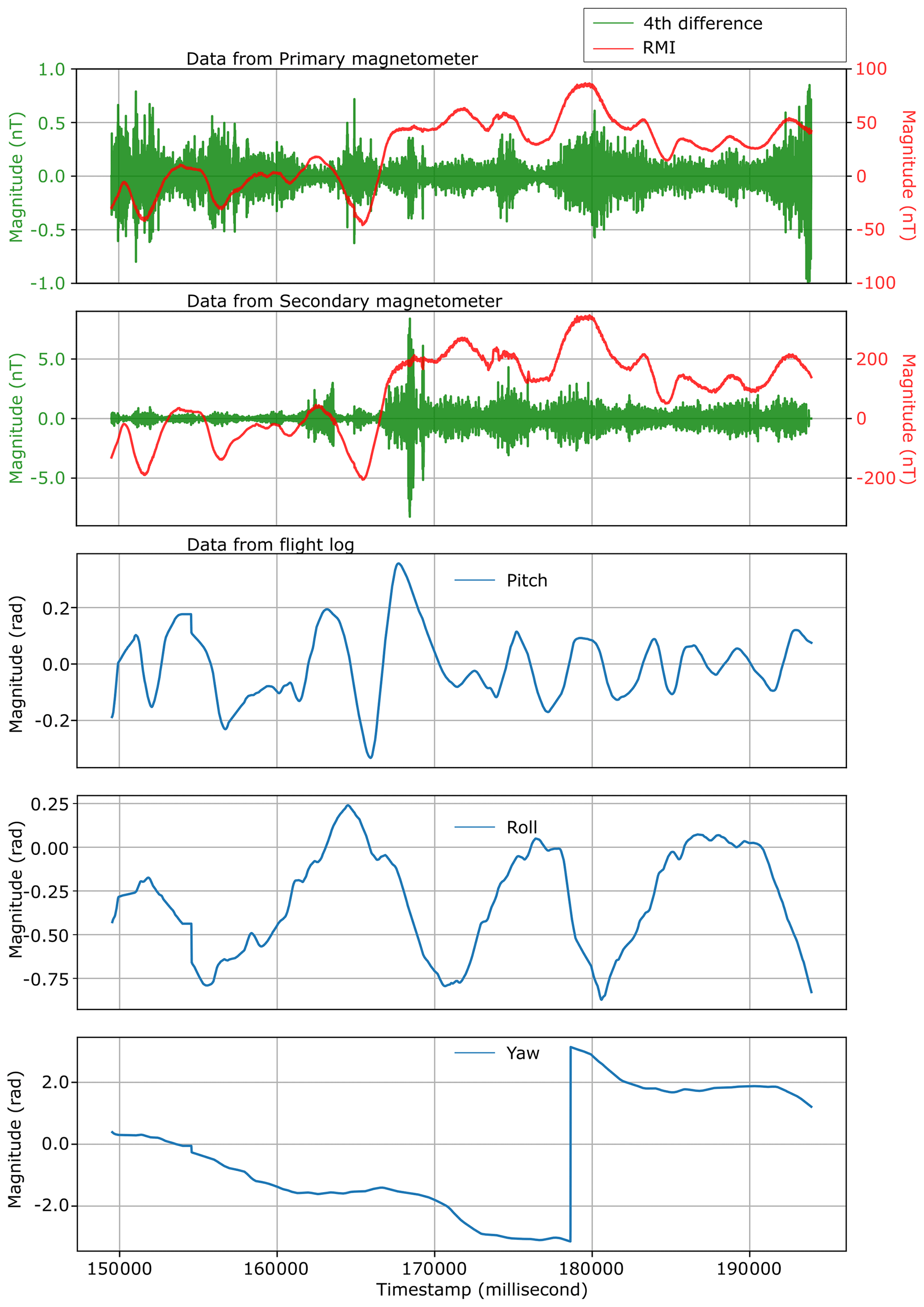
Furthermore, Figs. 12 and 13 present the RMI from both magnetometers and the current load from the battery monitored by the system in the flight from the take-off to the fixed-wing cruise, accompanied by their respective fourth difference. Take Fig. 12 for example – the first part of the RMI (outlined with dark grey box) was collected in the take-off phase (in the multi-rotor mode), whereas the rest was recorded in the fixed-wing cruise mode. The gaps inside each RMI profile were due to in-flight maneuvers of the UAV somehow rendering the magnetic field falling into the QTFMs' dead zone. The two RMI profiles in Figs. 12 and 13 are also visually identical, akin to the previous experiment. But the two profiles look visually smoother than those collected in the multi-rotor mode. Interestingly, a clear correlation between the RMI profiles and the output current from the battery, especially during the take-off phase, is observed. After transitioning to fixed-wing mode, there is a clear decrease in the current and the magnetic field. The magnitude of the two magnetic profiles in Fig. 15 are quite comparable before 170 000 ms, but after that moment the difference in the magnitude increases significantly, which means that the magnetometers are still highly susceptible to the inference from the UAV. The plots of the RMI in Fig. 15 show a visually clear correlation with the pitch. The fourth difference of the in-flight measurements of the primary magnetometer during the fixed-wing cruise is around ±0.2 nT (Fig. 15), slightly higher than the data collected before the take-off. It is evident that the fixed-wing mode gives less noisy data.

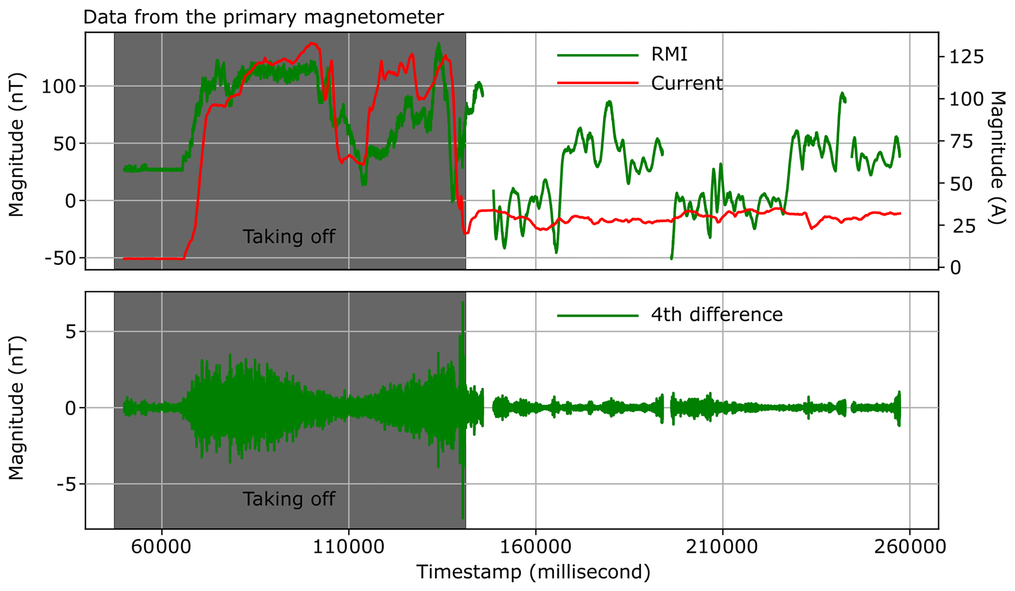
Figure 12 Data excerpt of RMI profile recorded by the primary magnetometer and its fourth difference, together with the profile of output current from the battery with d=20 cm and L=30 cm. The IGRF (50 563 nT) has been removed.

Figure 13 Data excerpt of RMI profile recorded by the secondary magnetometer and its fourth difference, together with the profile of output current from the battery with d=20 cm and L=30 cm. The IGRF (50 563 nT) has been removed.

Figure 14 The production flight of the data excerpt shown in Figs. 12 and 13. The altitude indicates the in-flight height above mean sea level.

Figure 15 The RMI of the second segment from left to right in Figs. 12 and 13 and the corresponding attitude from the flight log.

6 Discussion

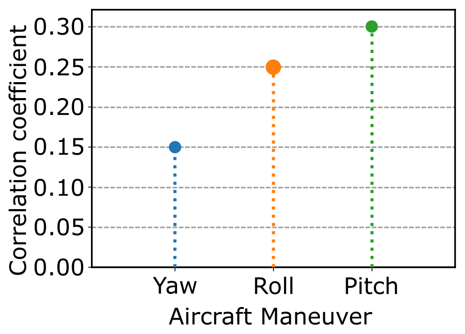
Based on the static and dynamic experiments, it is obvious that the magnetic interference from the platform is rather complex, especially when the platform is in flight. From the static magnetic interference mapping, we have acquired insights into some potential regions on the platform. However, solely measuring static magnetic signature is not sufficient to provide decisive information for the development of an airborne magnetometry system. It seems more practical to understand the interplay between the dynamic and complex magnetic interference when the platform is properly powered and in operation. For example, the static magnetic signature indicates that the interference at the primary and the secondary magnetometer is minimal and the longitudinal difference is less than 5 nT. This is because during the static magnetic interference measurement the major interference is due to the permanent magnets of the electric servomotors and electric motors. Once the platform is powered and flying in operation, magnetic interference increases significantly. The reason for the increase can be attributed to magnetic leakage of the electric servomotors and electric motors, the magnetic field generated by dynamically varying current flowing from the battery to the flight controller, and the magnetic interference due to eddy current in the airframe. Surprisingly, in comparison with the first dynamic experiment, the magnetic interference observed in the standby phase in the second dynamic experiment has also changed considerably. In principle, the longer boom provides increased distance to sources of interference, leading to a stronger attenuation of interference from the platform, but in the experiments the longitudinal gradient between the primary and the secondary magnetometers increased by 10 times over that in the first dynamic experiment. The first variable between the two dynamic tests is power consumption because the platform consumes much more power in the multi-rotor mode than in the fixed-wing mode, which leads to strong current in the cables. The second variable is the layout of the components inside the fuselage, such as the orientation of the current-carrying cables connecting the battery with the flight controller. The current-carrying cables are quite soft and can dangle with the aircraft's attitude along the longitudinal axis of the fuselage, which led to such a stronger correlation with the pitch (Fig. 16) other than the superimposition effects of all the maneuvers.

Figure 16 Correlation coefficient of the RMI and aircraft maneuvers.

Regarding the issues that have been discovered, we will try to further increase the distance between the magnetometers and the platform without compromising the flight stability because the noise envelope is too high at the moment to meet the industry standard for mineral exploration. Secondly, the cables connecting the battery with the flight controller should be properly placed and shielded to further reduce the interference.

7 Conclusions

We presented a static experiment, and based on the assessment of the results of the static experiment we proposed a front-boom mounting system, the stability of which is supported by our aerodynamic simulations. Following this, we conducted two dynamic experiments to assess in-flight noise in operation. The results are insightful because the strongest interference surprisingly originates from the cables connecting the Li-Po battery to the flight controller. As a consequence, we propose to further increase the distance between the magnetic sensors and the UAV. Additional noise-reduction measures include shielding the cables causing strong magnetic interference and relocating the UAV's wiring harness.