A towed magnetic gradiometer array for rapid, detailed imaging of utility, geological, and archaeological targets

Efficient and accurate acquisition of magnetic field and gradient data have applications over a large range of environmental, archaeological, engineering, and geologic investigations. Developments in new systems and improvements in existing platforms have progressed to the point where magnetic surveying is a heavily used and trusted technique. However, there is still ample room to improve accuracy and coverage efficiency and to include reliable vector information. We have developed a vector magnetic gradiometer array capable of recording high-resolution field and gradient data over tens of hectares per day at 50 cm sensor spacing. Towed by an all-terrain vehicle, the system consists of eight vertical gradiometer sensor packages and incorporates differential GPS and an inertial measurement system. With a noise floor of around 6 nT at 15 km/h towing speed and 230 Hz sample rates, large areas can be mapped efficiently and precisely. Data are processed using a straightforward workflow, using both standard and newly developed methodologies. The system described here has been used successfully in Denmark to efficiently map buried structures and objects. We give two examples from such applications highlighting the system's capabilities in archaeological and geological applications.

1 Introduction

Ground-based magnetometry has been a staple for environmental geophysics for decades. The method has enjoyed extensive use in unexploded ordnance (UXO) (e.g. Billings, 2004; Barrow and Nelson, 1998) and archaeology (e.g. Linford et al., 2007), with a number of other additional applications such as utility detection, geologic investigations, environmental surveys, and engineering studies (Nabighian et al., 2005).

In many cases, simple but accurate detection of a large anomaly is sufficient, for example finding capped, abandoned wells (Kaminski et al., 2018). Other applications, such as in multipole expansion in UXO discrimination (Sanchez et al., 2008) or detailed archaeological investigations, require densely sampled data of high quality. Often, the area of interest in these surveys is large, requiring an efficient acquisition scheme.

There are many commercial turn-key magnetometer systems available, both in total-field and gradient configurations. Most systems (e.g. Geometrics 858, Sensys MXPDA, or Gem Systems GSM-19) utilize Overhauser (Hrvoic, 1989) or alkali (often caesium) vapour (Hardwick, 1984) total-field sensors; i.e. the sensors measure the scalar magnitude of the magnetic field. This has the benefits of providing stable, absolute measurements insensitive to sensor orientation when measuring the magnetic field and minimally sensitive when measuring the total vertical gradient, i.e. the vertical gradient of the total field, or TVG. Other systems, like the US Geological Survey TMGS system (Bracken and Brown, 2005) or the Foerster Ferex (https://www.foerstergroup.com, last access: 26 November 2021), use fluxgate sensors (Gavazzi et al., 2016), which are inherently vector sensors and have a lower power consumption relative to traditional alkali vapour systems.

In principle, any of these systems can be mounted to a vehicle or towing platform with a bit of engineering creativity if not built as such. Towing a magnetic system, whether total field or gradient, has obvious advantages to acquisition speed and ease. No longer limited to walking speed, spatial coverage of an area of interest can be expanded dramatically in areas accessible by vehicle. However, careful calculation and removal of the self-gradients from the vehicle are required.

We have developed a new vector magnetic gradiometer array (tMag) designed for near-surface geologic, environmental, and engineering applications to complement the existing, available instruments. The tMag system strives to provide efficient and high-resolution mapping of magnetic field and gradient data from a towed platform: tens of hectares a day at 50 cm line spacing with a noise floor of approximately 8 nT/m while moving.

The tMag design differs from many other systems in two critical ways; first, the system was designed from the start to be towed rather than modified for vehicle mounting, and second it utilizes commercially available fluxgate vector magnetometers rather than total field. Additionally, the sensors have a high sample rate. These features coupled with completely custom acquisition and processing software allow for a flexibility not generally available in commercial systems.

By designing the platform from the start to be towed, we had the ability to move the majority of the electronics over 10 m away from the sensors, significantly reducing bias noise. Being towed also allows flexibility in the towing vehicle, as a modular part of the whole system, requiring only a tow hitch and no special modifications. Smaller and more nimble vehicles, such as an all-terrain vehicle (ATV), improve site access and create a smaller magnetic footprint.

Utilizing vector magnetic sensors looks forward to the construction of the full gradient tensor (all spatial derivatives of the magnetic field), while still providing the standard data components available in other systems. The derivatives provide additional data component maps for direct interpretation that highlight different features, such as edges, as well as increasing the data available for inversions and other interpretation techniques.

We describe the tMag system design and data workflow scheme. Specifically, we discuss design specifications, as well as discussing optimal acquisition parameters. We then discuss all aspects of the workflow, from system calibration through data processing, including looking forward to accurate construction of the full tensor gradient. We present a successful archaeological mapping example from Ørregård, Denmark, to demonstrate the system capabilities.

2 The tMag system

We designed the tMag system to utilize the capabilities of a vector magnetic array to potentially construct all components of the magnetic gradient tensor, while keeping the noise levels from system electronics, the towing platform, and motion as low as possible. A key performance indicator was to reliably identify anomalies down to 8 nT/m total vertical gradient amplitudes from a towed platform based on specific anomalies we expected to encounter and a 20 km/h driving speed. In addition, we desired efficient mapping, with the goal of several tens of hectares mapped per day at full coverage, i.e. no gaps between lines. We achieved these goals through a detailed engineering system design, particular attention to noise sources, and with careful calibration and data processing techniques.

2.1 System description

The tMag system comprises an array of eight vector magnetic gradiometer sensor packages, each with two three-component fluxgate sensors arranged in a vertical gradient configuration, resulting in 48 independent measurements. We use commercially available fluxgate sensors from Bartington Instruments (Grad-13, https://www.bartington.com/grad-13, last access: 26 November 2021), with a customized data logging platform. Figure 1a shows the physical configuration of the system, with Fig. 1b showing a systems collaboration diagram. In Fig. 1a, each of the eight Bartington sensors can be seen as a white tube, rigidly holding the two sets of vector sensors 1 m vertically separated. Each sensor package contains an independent analog-to-digital converter and returns a digitized data stream to a multiplexer on the ATV.

Fluxgate sensors provide multiple advantages to proton precession, alkali vapour, or Overhauser systems. The simpler, solid-state design is more robust and can provide vastly higher sample rates with relatively low power draw, though we note the newest generation of total-field sensors may match or exceed the fluxgate power and sampling performance. Most significantly, the sensors are naturally vector sensors (when used in sets of three), coupling only to one component of the magnetic field. The use of fluxgate sensors, however, requires periodic calibration and bias correction during processing, detailed below.

In addition to the magnetic sensors, the array contains a system for positioning and attitude measurement. Two GPS units are mounted on the frame for accurate position and heading estimation, while an inertial measurement unit (IMU) records yaw, pitch, and roll of the frame.

The output from all magnetic sensors, GPS, and IMU are transmitted by cable to the recording electronics, mounted on the ATV. This eliminates any electronic noise on the sensor platform from the recording electronics and computer system.

2.2 Design aspects

The instrument packages are mounted on a towed sled, consisting of a wooden platform and front shield to protect the sensors from rocks and debris, a fibreglass frame system for rigid support, and three polyethylene (ultra-high molecular weight for durability) sled runners to provide as stable a platform as possible. All brackets are non-metallic and 3D printed in a carbon-fibre-enforced plastic material, with bolts and nuts made of nylon. The sled system is 3.75 m wide by 1 m. It is rigid, without suspension, as discussed in further detail below, and is easily transported on a long trailer.

2.2.1 Sensor and electronics configuration

The eight gradiometer packages (each comprising two, three-component magnetometers in a vertical gradient configuration) are mounted 50 cm apart, perpendicular to towing direction, allowing for full definition of total-field anomalies from sources as shallow as 25 cm and gradients at 50 cm. Each is aligned with the x axis facing the driving direction, the y axis to the right, and the z axis as positive downward. The bottom sensors are 15 cm above ground level, with 1 m between the top and bottom sensors (Fig. 1a).

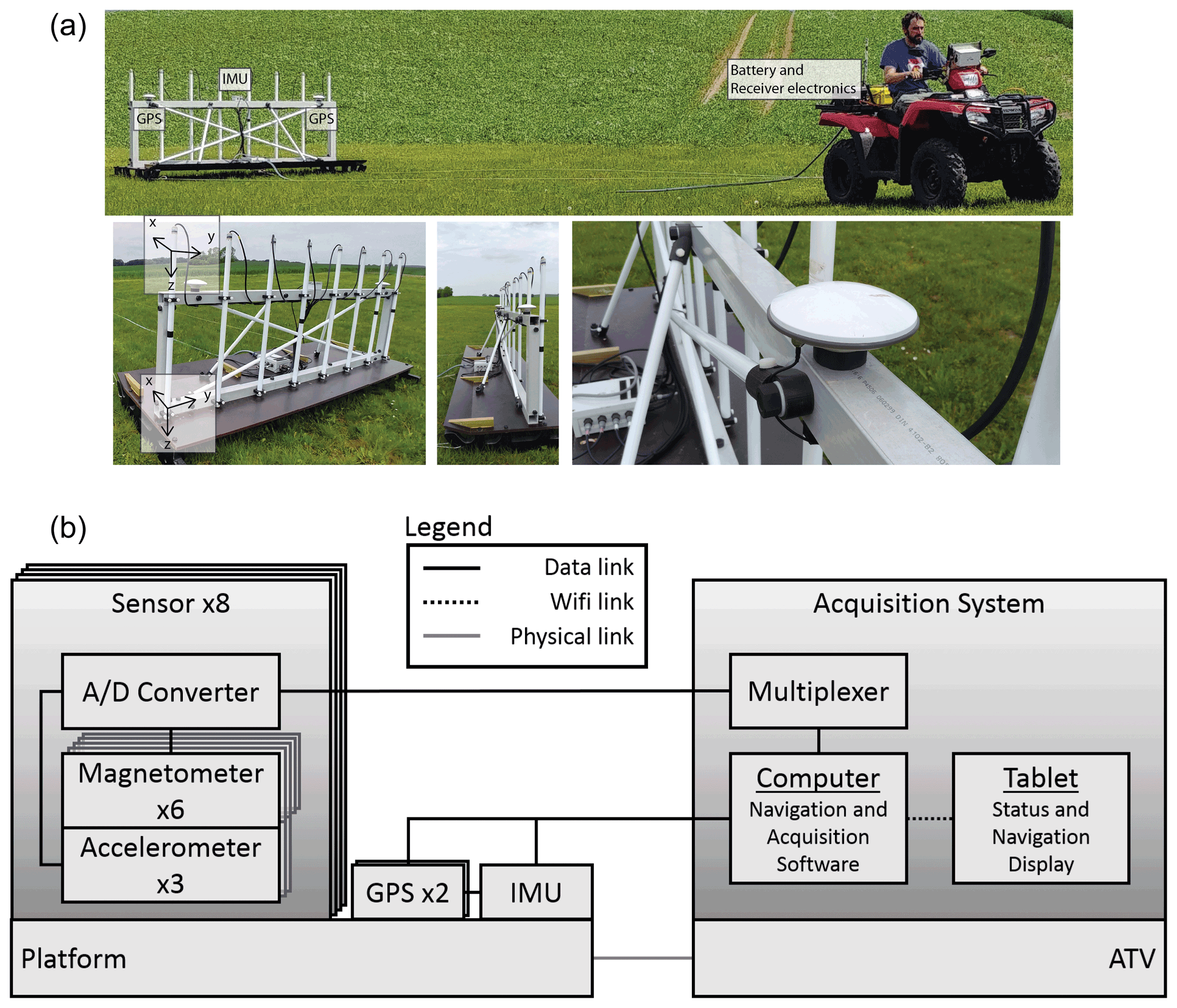
Figure 1 (a) tMag system. GPS and inertial measurement units labelled. Vectors indicate approximate sensor position and orientation. (b) Systems collaboration diagram for the tMag system.

In order to eliminate noise from the acquisition electronics, the data logging and control system as well as the power supply are mounted on the towing vehicle, 10 m ahead of the sled – the exact distance necessary is dependent on the towing vehicle, but in our case the contribution of the ATV to the total vertical gradient was statistically insignificant past 7 m. The logging and control system consists of a multiplexor to accommodate the high-throughput data streams from the eight gradiometer packages, which interfaces with an Intel NUC PC, also mounted with the electronics system. Figure 1b shows a systems collaboration diagram, showing the interconnected elements.

The GPS and IMU units are mounted to the frame, in as close to a null coupling position as possible. Various locations were tested, with the final location chosen for both stability and to minimize the induced magnetic signal given the requirement that the sensors must be rigidly mounted on the frame. Any coupling from induced alternating currents is filtered or aliased out, while the small DC contribution is removed by the bias corrections.

2.2.2 Positioning and attitude measurement system

Two GPS units (Tersus BX316) are mounted 2.4 m apart on the frame (Fig. 1a). These units are fully post-processing kinematic (PPK) compatible with a third unit, set up as a base station near the survey area. The two units are interfaced to report heading information in real time. The binary data stream reports positions at 5 Hz with all information necessary for post-processing the differential corrections.

An IMU (Redshift Labs UM7 attitude and heading reference system) is also positioned on the frame to record yaw, pitch, and roll utilizing a system of three-component gyroscopes, accelerometers, and magnetometers incorporated with an extended Kalman filter. This information is recorded at 30 Hz as quaternions for correcting the magnetic data during the processing workflow. The IMU receives direct, real-time GPS input through a separate connection to improve heading estimate accuracy and provide accurate timing.

2.2.3 ATV setup

The ATV is positioned 10 m ahead of the acquisition platform or 10.5 m ahead of the sensors themselves. The sled is pulled with three tow ropes, with the power and sensor cables protected in a hose adjacent to the central rope. The distance was selected to eliminate the signal contribution from the ATV to the total vertical gradient component below the noise floor while still allowing for safe towing. We note that a larger ATV (such as a two-seat side by side) may have different noise characteristics and require re-evaluation of the required distance.

The entire system is powered by one lithium-ion 12 V, 100 Ah battery bank, providing ample power for a day of acquisition. The PC mounted in the receiver electronics is controlled by a tablet via Wi-Fi and a remote desktop connection.

2.3 Acquisition parameters and data recording

The sensor data from the magnetometers and positioning system are recorded at a variety of sample rates and file types to maximize efficiency (Table 1). The various data streams are logged with custom software, MagLog, running on the mounted PC.

Table 1 Maximum and nominal sample rates for each sensor system.

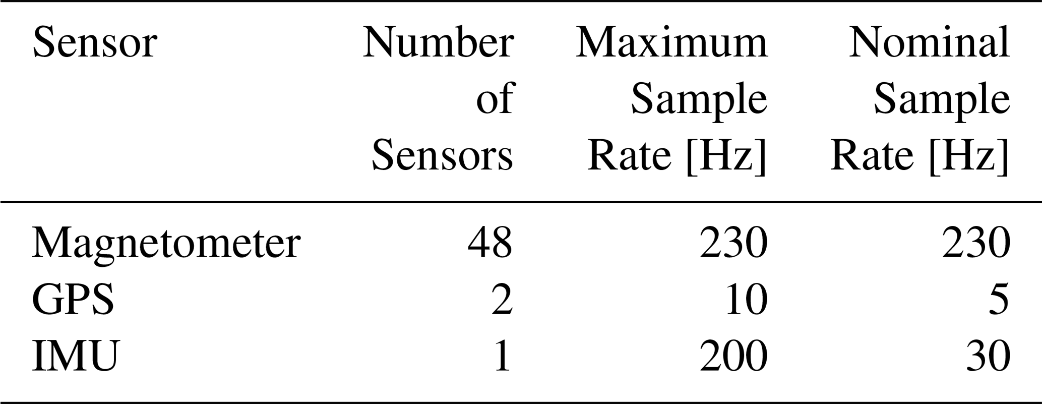
Each of the eight gradiometer packages reports an independent data stream at a user-defined sample rate of up to 230 Hz via an RS-485 interface, which is collected by a multiplexor and delivered via Ethernet cable to the PC. The individual data packets reported by each gradiometer consist of the readings from each of the six magnetometers, plus a unique packet number and a checksum value for error checking, resulting in an 81-byte packet. This yields over half a gigabyte of data per hour at the full sample rate.

2.4 Standard survey procedures

For many archaeological and UXO applications, full sensor coverage is desired; that is the distance between lines should be the same as the distance between sensors on the platform, resulting in an effective line spacing of 50 cm. This follows from an oft-used rule of thumb in magnetics: that the line spacing should be no more than twice the depth to the target (Reid, 1980). When performing such a survey, the subsequent 4 m line spacing requires a “racetrack” or “sequential looping” acquisition approach, rather than attempting to turn a sled with a 10 m tow cable. For a roughly rectangular survey area, the survey begins with an acquisition line along the long edge of the area of interest, turning 90^∘ and continuing to the middle of the short edge, proceeding back down the middle of the area, and turning to complete a large “oval” pattern. The next line proceeds immediately adjacent to the first, continuing in the same direction and completing a second oval. This continues in sequence, creating a pattern that fully covers the area without requiring sharp turns.

To assist with mapping, the operator has a tablet mounted on the ATV, interfaced to the PC. Along with the logging software, the PC also runs Aarhus Navigator, an in-house developed navigation system, which provides a real-time map showing acquisition lines, any GIS background maps, current and past position of the ATV, driving speed, etc. The user can select to monitor one or more data streams as well.

The survey can be conducted with one field operator. However, we generally operate as a two-person crew (and suggest doing so) for safety. We find the greatest efficiency when one operator runs the instrument while the other secures site access in the area.

Over time, the gimbals in the IMU drift and must be re-zeroed every 3 to 5 min to ensure accurate attitude estimates. The procedure is nearly instantaneous but requires that the platform be held still. We pause at the end of every third or fourth line and allow the gimbals to zero.

3 Data processing

The data processing scheme is designed to highlight isolated targets and avoid Fourier-domain operations, which can introduce artefacts and potentially obscure anomalies of interest. All steps are performed on the data as recorded; the data are only gridded for visualization as a final step. The workflow can easily be modified, however, with any standard magnetic processing technique such as upward continuation (Blakeley, 1996) or levelling (Mauring et al., 2002) if tie-lines are acquired, should it be desired, taking care that they are incorporated properly. For example, upward continuation cannot be done on a line-by-line basis and would benefit from calculation in a 2D Fourier domain. The modular workflow begins with completely unprocessed data and so can be tailored to any processing approach.

3.1 System calibration and timing

The system is periodically calibrated for magnetic sensor gain and IMU heading. In principle, the sensor gain need only be recalculated when the sled is modified; however we periodically recalibrate for quality control, approximately once per month during “field season” when the system is in common use. We have not observed drift on any scale in the magnetic system gains.

Sensor gain values must be determined in a magnetically quiet region, ideally in an area with a constant magnetic field. To overcome small variations in the local field, we acquire a large amount of calibration data and solve for the values in a least-squares sense. We set up a vertical gradiometer (Geometrics 858) near the field site as a base station with the two total-field sensors at the same heights as the sensors on the array. The array is driven in a large figure of eight pattern, keeping the tow rope as straight as possible behind the ATV – a radius of 75 m is sufficiently large. This figure of eight is repeated several times and in opposite directions and ideally rotated 90^∘ and done again (a clover-leaf pattern). In post-processing, each three-component magnetic sensor on the array is calibrated to the corresponding base station sensor, computing an individual gain for each of the 16 sets of three-component magnetometers. The gain factors on each of the three components should be equal (Olivier Masseglia, Technical Director, Bartington, personal communication, 12 April 2018). Figure 2 shows an example of data before and after calibration. The gain factors can be up to 10 % (Olivier Masseglia, Technical Director, Bartington, personal communication, 12 April 2018) though are closer to 2 % per sensor.

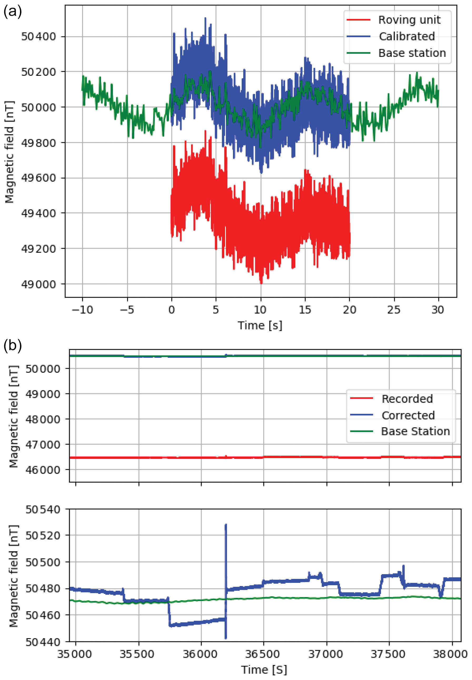
Figure 2 Demonstration of gain correction for a synthetic case (a) and field calibration (b). The steps seen in the blue curve in (b) correspond to changes in heading in the system, indicating heading-induced biases corrected during processing.

The IMU magnetometers are calibrated in a similar manner, with the additional step of tipping the system to horizontal several times to rotate the magnetometers as much as possible. The IMU software then automatically computes gains and biases, and all computed yaw, pitch, and roll values are relative to magnetic north.

Each of the eight gradiometer packages has an on-board A/D converter, with an independent non-controllable timing system and with data transmitted in packets. In other words, the data streams cannot be started synchronously, but the individual samples in a data stream are accurate to the accuracy of the A/D converter. To obtain a sufficient accuracy of the timing between the data streams from each A/D, GPSs, and IMU a real-time timing correction algorithm was developed resulting in an estimated accuracy of the data streams of 10–20 ms. This is sufficient in the subsequent data processing algorithms.

As mentioned, the system calibration is not a regular procedure in contrast to the standard processing steps outlined in the following paragraphs.

3.2 Geometric correction

The first step in a standard processing flow is to correct the positions of the sensors relative to the GPS. The GPS times are first linearly interpolated onto the sensor observation times, with the position subsequently also interpolated. The position of each sensor package relative to the GPS is computed as a function of heading. This yields an estimated position for each magnetic observation. Note that this requires accurate synchronization between the GPS timing and the sensor timing.

3.3 Bias correction

In addition to a gain, each of the 48 sensors has an individual bias that must be computed. This bias does change on a daily basis, essentially every time the system is moved in an area of high magnetic gradient, e.g. onto a trailer and therefore needs to be established regularly. The bias can be directly measured by recording data before and after rotating each sensor 180^∘ around each axis; this, however, requires the entire platform be turned upside down and is therefore not practical. We instead approximate the biases in post-processing.

We use an iterative, windowed process to return the data to zero mean. Simply subtracting the mean from the data could be severely influenced by large magnetic anomalies in the survey area, and removal of either the mean or median from the entire line could be affected by lines not perfectly straight, so we remove large standard deviations in an iterative process. We divide each line of data into half-overlapping windows of 30 m width and remove all data more than 2 standard deviations away from the mean. We then recompute the mean and iterate four times within each window. A second-order polynomial is fit to the computed means, which is then subtracted from the data. Figure 3 shows an example of a single line of data with four sensors before and after bias removal. We note that after bias removal, levelling is generally not required. Figure 3 clearly shows the mean has been removed from the data; more subtle long-period variations on the order of several nanotesla have also been removed.

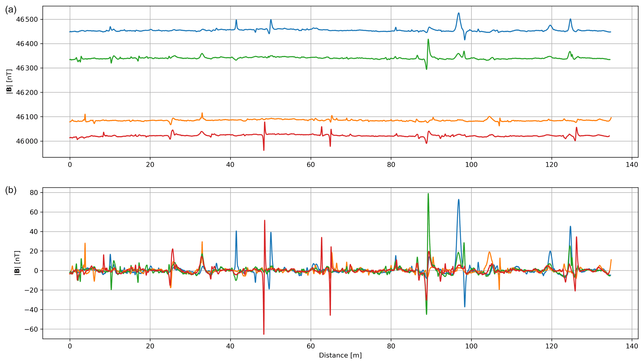
Figure 3 Example of a line of total-field data from four representative sensors before (a) and after (b) processing with bias correction. The data values have been iteratively set to zero mean, discounting values more than 2 standard deviations away. The windowed approach additionally removes longer-period variations.

3.4 Power line removal

Power line noise linearly adds a 50 or 60 Hz (plus harmonics) signal to the recorded data. This signal varies with proximity to the power line, as well as from variations in the power grid itself. We remove this contribution through a model-based approach as detailed in Kass et al. (2021) and summarize the procedure here. We use a windowed, model-based fitting of a 50 Hz signal and harmonics to estimate and subtract out the contribution from power lines. Windowing the data is critical, as not only does the amplitude of the signal change with proximity to the source, but the power line characteristics are also not constant; there are slight variations in the frequency and amplitude. We therefore define a temporal window, 0.25 s in this case, where the amplitude, phase, and frequency of the signal are assumed to be constant. We solve for a best-fitting 50 and 100 Hz harmonic set of sinusoids for each window with amplitude, phase, and frequency as free parameters. We add a constraint that each parameter must vary smoothly between windows using Tikhonov regularization (Hansen, 1998). Synthetic and field examples show that more than 98 % of the power line signal can be removed with this method, without the need for filtering operations, which may distort the frequency content of the data. Figure 4 shows an example dataset before and after harmonic removal. The power line signal is almost completely removed except in the area of the most severe contamination, while leaving the anomaly undisturbed. We prefer to compute and remove the signal from the total-field and gradient data to avoid error accumulation; however the procedure can be applied to individual vector components before calculation of the derivative products if desired.

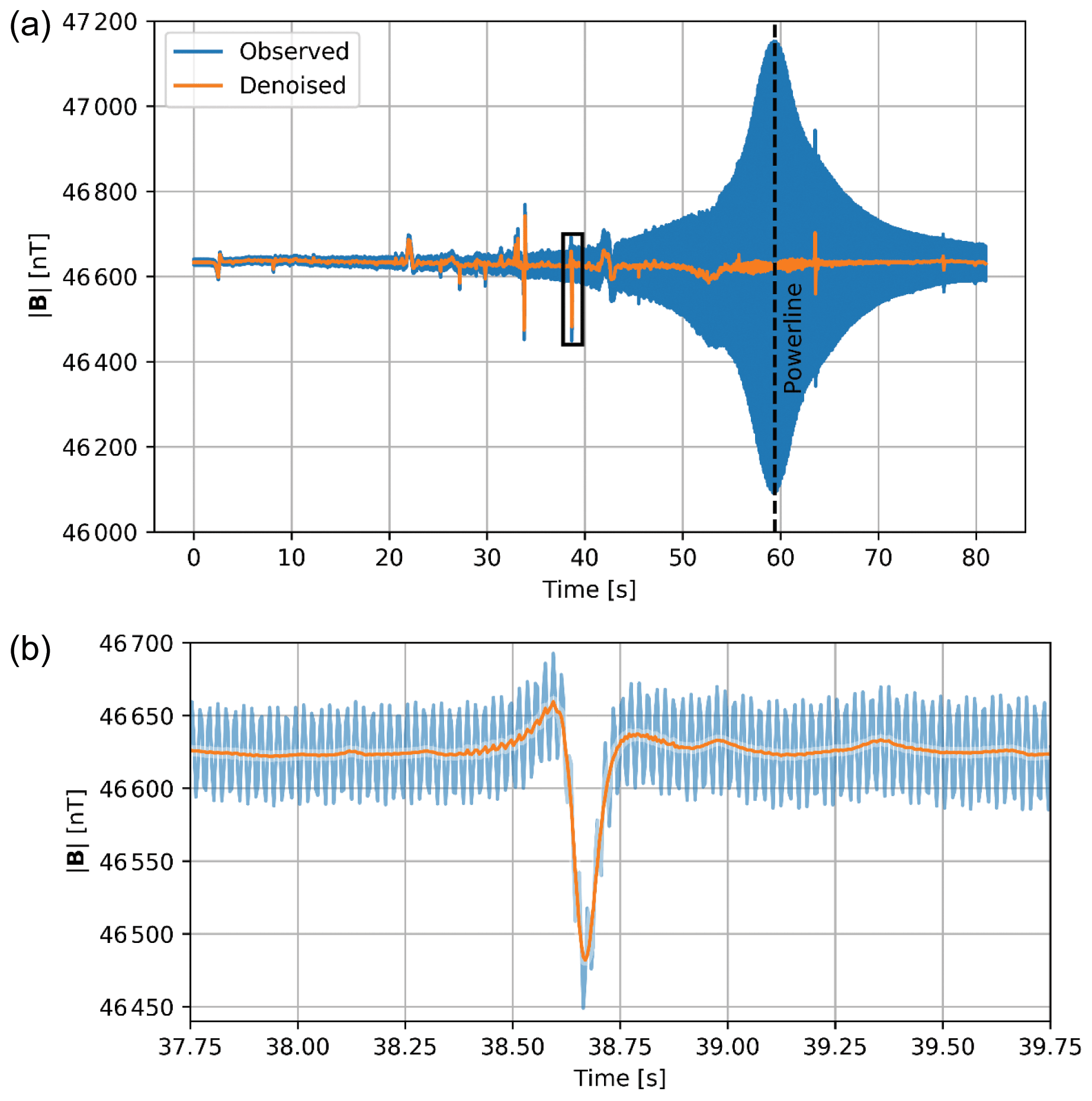
Figure 4 (a) Example of a line of total-field data acquired beneath a power line before and after power line removal. In total, 98 % of the power line signal is removed. The black box indicates the zoomed area in (b). (b) Zoom on 2 s of data.

3.5 Attitude correction

While total-field magnetic data are insensitive to orientation of the sensor package, the vector components are critically dependent on the attitude of the acquisition platform. Figure 5a shows the effect of pitching and rolling the sensor: for a survey in Denmark, just 6^∘ of roll can induce 2000 nT of error into the measurement. We therefore use the data from the IMU to rotate the vector components back to a common coordinate system, regardless of the heading of the instrument.

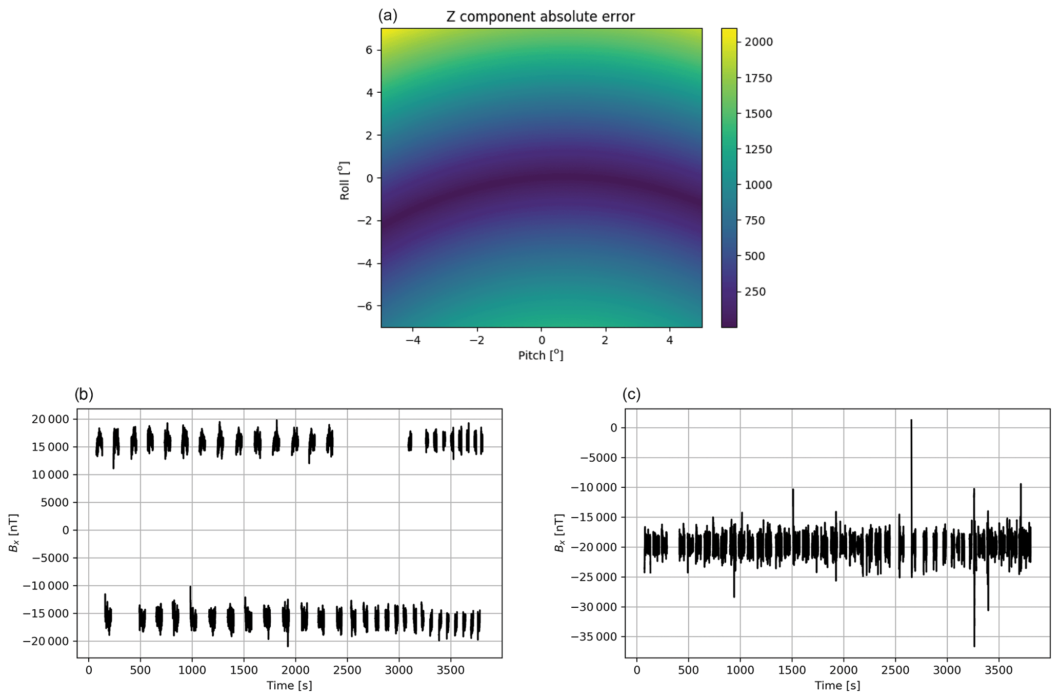
Figure 5 (a) Example of the error (nT) introduced in magnetic vectors due to roll of the platform for a survey at Danish magnetic latitudes. For example, 6^∘ of roll can contribute 2000 nT of signal to the y component. (b) Example x component of the data presented as a time series for an entire survey. Each block of data corresponds to one line (i.e. driving direction), showing how the x component of the field is primarily controlled by driving direction. (c) The same data after correction with the inertial measurement unit. The data have been rotated to a common coordinate system from relative to the acquisition platform.

The attitude of the acquisition platform is recorded as quaternions, a four-component vector consisting of three imaginary and one real component (Hamilton, 1866). Quaternion algebra defines a matrix multiplication that rotates the observed magnetic vector back to a common coordinate system in a single operation. As an example, Fig. 5b shows the data for a single sensor, in this case the x component of one of the bottom sensors, over an entire survey. Each “block” of data corresponds to a single line. In this case, the x component is aligned with the driving direction and therefore alternates between each line where the system was driving either north or south. In effect, the sensor is acting as a compass. Figure 5c shows the data after incorporation of the IMU data. The x component is now no longer the driving direction but rather is aligned with grid north. Not only the gross effect of heading is removed but also the smaller changes in orientation as the system moves over rough terrain. Pitch and roll are generally less than 5^∘ in a survey, limited mostly by ATV safety though may exceed this number for short periods due to vibration or jostling.

3.6 Calculation of derivative components

The system records individual vector components. For each gradiometer package, a total-field measurement is computed from the vector sensors for the top and bottom set; the total field is simply computed as the square root of the sum of the squares of each component. The total vertical gradient is computed as the difference between the bottom and top total-field sensors divided by the 1 m distance.

3.7 Visualization

Only at the final step are data gridded for visualization. Any appropriate algorithm can be used; we use an inverse-distance weighted (IDW) approach for efficiency, given the large number of data points. Data are generally gridded to 25 cm with the inverse distance weighted to a power of 2, but these numbers can be adapted given specific survey conditions.

4 Examples

We demonstrate the capabilities of the tMag system with two field examples from archaeological investigations in Denmark: Ørregård and Aggersborg.

4.1 Ørregård, Denmark

The Ørregård area covers an Iron Age settlement, which has been studied in detail by the Herning Museum and others. The settlement itself has archaeological significance as an anomalously early example of a hypothesized military production facility, possibly with Roman inspiration (Sommer, 2017). Of key interest to geophysicists is the large concentration of iron kilns, providing large geophysical anomalies in addition to the more subtle anomalies associated with the settlement buildings.

The data were acquired using the standard procedure described above to achieve full spatial coverage. Acquisition of the entire survey field, approximately 4.5 ha, took slightly under 3 h from arrival to departure, including equipment setup and breakdown. For comparison, a walking survey was previously performed here which took nearly 3 weeks. Data were processed with the previously described workflow.

Figure 6a shows the total-field data for a section of the survey area, while Fig. 6b shows the corresponding TVG map. A variety of archaeological structures are visible in both datasets; as the TVG is a derivative of the total field, the anomalies are sharper than expected but decay in amplitude faster.

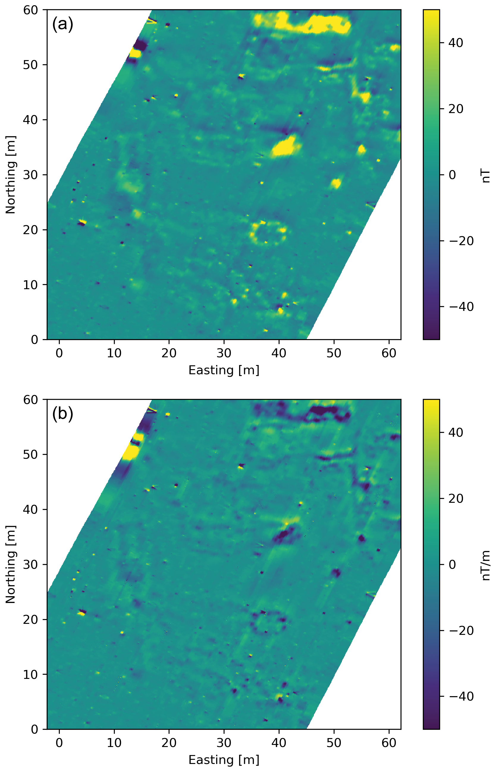
Figure 6 (a) Total-field data from Ørregård, Denmark, showing archaeological anomalies. (b) Total vertical gradient data from the same area.

There are two general sources of archaeological anomalies in the region: those from presumed iron production and those from the rest of the settlement. These sources result in a bimodal distribution of anomaly strengths: from 50 to 100 nT and the lower amplitude anomalies in the range of 10 nT. The longer linear, lower-amplitude anomalies correspond to a road, with some of the features seen to the north representing structure foundations.

Some striping along acquisition lines is still visible in the higher-amplitude regions; the asymmetric nature of the anomalies can be controlled by the bias correction process but not completely eliminated as there will always remain a slightly asymmetric signal biassing the mean estimation. Fine-tuning of the algorithm can improve the result slightly but with diminishing returns.

Figure 7 shows a spectrogram of the recorded noise at this field for 60 s of data both stationary (panel a) and moving (panel b). Note the noise level while moving is relatively flat across the spectrum.

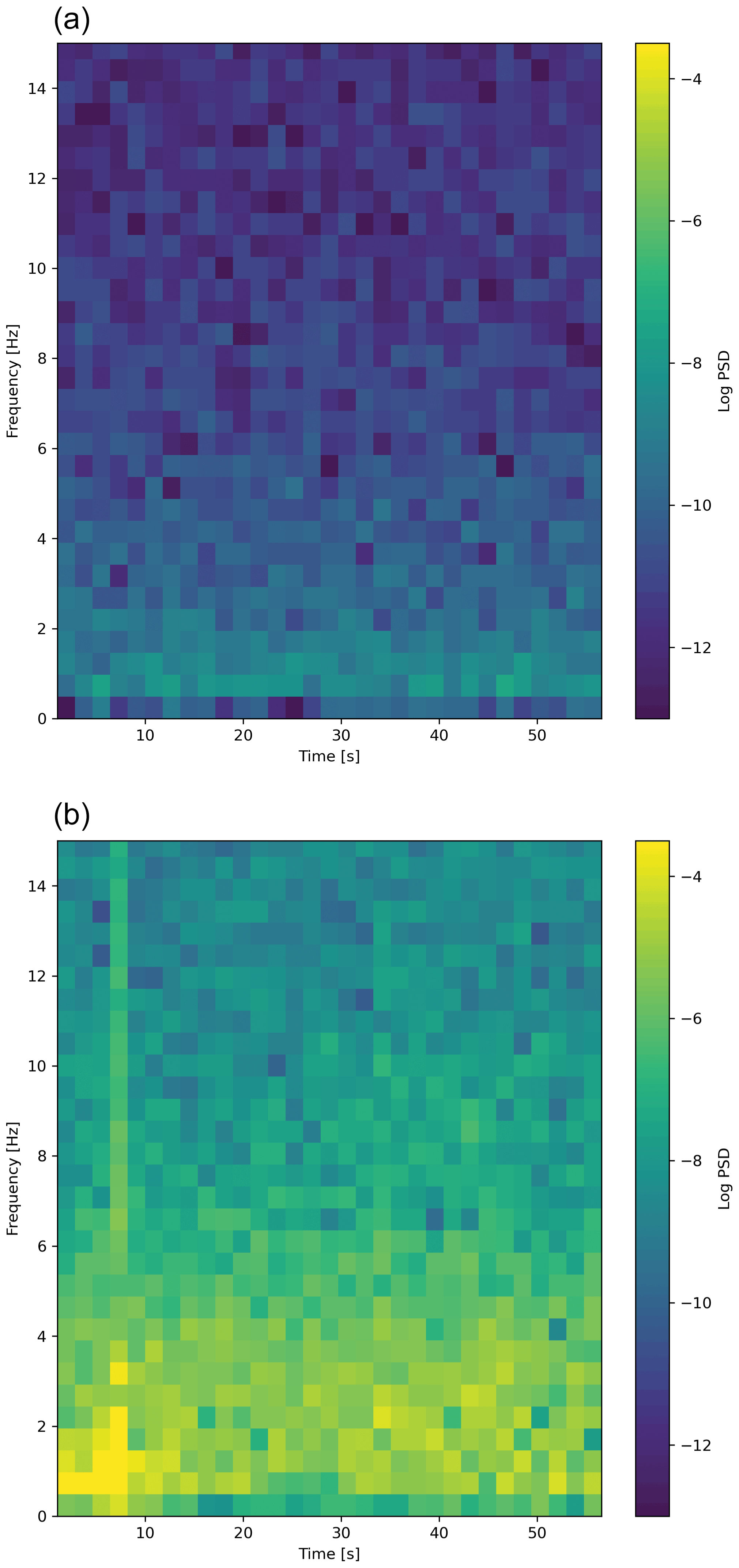
Figure 7 Spectrogram (log of power spectral density, PSD) of recorded vertical component data (B_z) for 60 s of stationary (a) and moving (b) records. The spectrum generally has power concentrated in the lower frequencies, and at 8 s the effect of a “bump” can be seen.

4.2 Aggersborg, Denmark

The Aggersborg archaeological site comprises Denmark's largest Viking ring fortress as well as buried villages outside the fortress proper. The site has seen at minimum three stages of construction: a Viking Age village, construction of the ring fortress by Harald Blåtand, and a later medieval construction and occupation period (Brown et al., 2014). Expected magnetic sources include isolated metallic artefacts, potential house foundations, and other construction using local materials. We performed a reconnaissance survey in the areas surrounding the fortress to identify any potential regions of interest for possible investigation later.

The surveys were conducted over 2 d, yielding approximately 80 line kilometres of data (or equivalent to 640 line kilometres of sensor data with all eight sensors), resulting in full 50 cm cross-line sensor coverage. Data were processed as described above.

Figure 8 shows the resulting total vertical gradient data for a subset of the area. In addition to compact anomalies, the map clearly shows periglacial features resulting from a type of permafrost polygon in sloping soft sediment or parallel to a paleo-shoreline (Davis, 2001). These features are a consequence of transported material with different magnetic properties than the surrounding soil infilling gaps left from melted ice wedges.

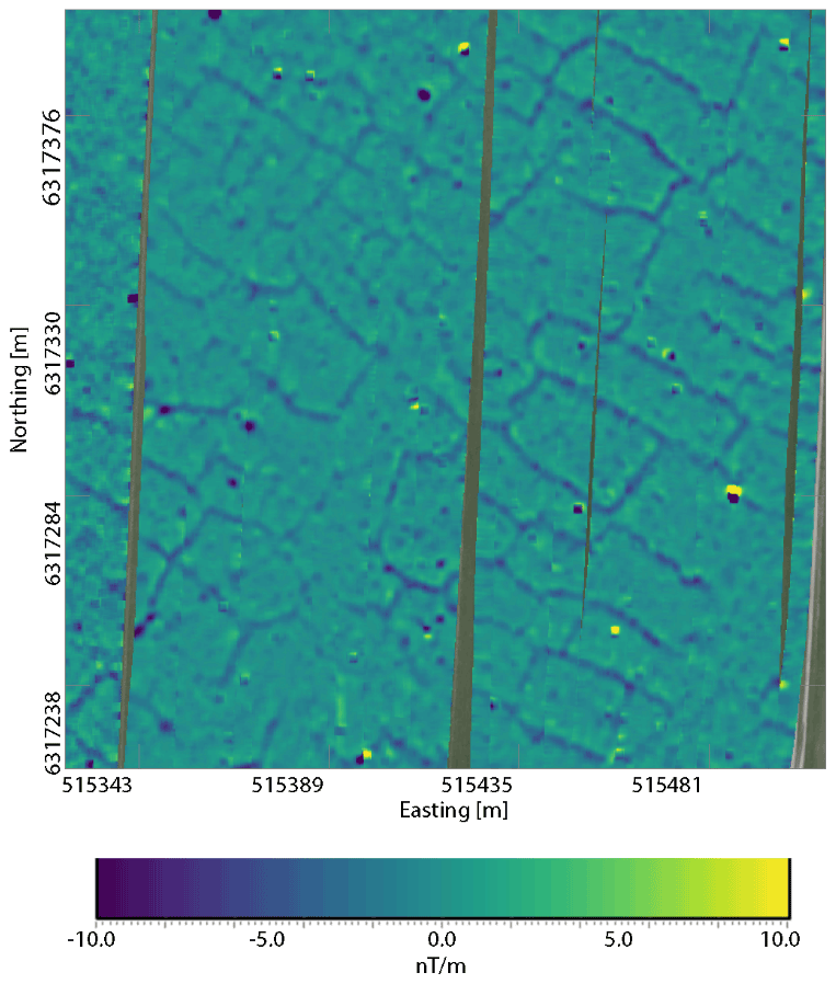
Figure 8 Total vertical gradient map in nT/m from Aggersborg, Denmark. Periglacial features can be seen as the polygonal background pattern, with a variety of compact anomalies of various shapes and magnetization visible.

5 Discussion

Noise levels for each sensor are slightly below 1 nT standard deviation at the full sample rate of 230 Hz when stationary (measured at multiple, rural locations, with the ATV engine idling). This value also matches published noise levels on the manufacturer website. Depending on terrain and driving speed, the noise floor is between 3 and 6 nT at 15 km/h based on repeated tests over multiple lines of data. Total vertical gradient standard deviations are approximately 6 nT/m, depending on terrain. We do not exceed 20 km/h with this system for both human and equipment safety. We did not observe significant drift as a function of temperature; however the temperature ranges under which the system has been used were quite small.

Our initial prototype of the system included a suspension system, whereby the central frame containing the sensors was isolated using elastic straps. We found that this introduced severe motion noise in the 10 to 20 Hz range, despite tension adjustments. With the high sample rate and desired spatial resolution, this noise was unsatisfactory. After trialling a second, rigid prototype, we found that a rigid system on a sled had superior noise characteristics. We therefore abandoned the suspension in favour of a simpler approach.

The bias correction works well as a high-pass filter, removing not only bias between sensors but also long-period variations. This procedure is well-suited to near-surface target detection, but should not be used for investigations looking at variations in all but near-surface geology.

For smaller, shallower targets, a shorter vertical separation may be beneficial due to the rapid decay of the vertical gradient and the reduced effects of pitch and roll of the system. If designing a new instrument based on this concept, additional modelling incorporating the recorded motion from this platform could assist in the selection of sensor separation.

This system is well-suited to mapping large open areas, such as fields, or wide areas such as roadways. The long separation between the vehicle and sensors does restrict the turning radius somewhat, so we would not recommend mapping in forested areas, for example. While 6 nT/m is a higher noise floor than that of carried or hand-pushed systems, we note that slowing acquisition speed can reduce the noise level at the expense of aerial coverage. However, for many archaeological and infrastructure applications, 6 nT/m is more than adequate. Understanding the potential targets is critical for planning this or any other geophysical survey.

The accuracy of the attitude correction is completely dependent on the accuracy of the IMU. The IMU we have employed has a stated accuracy of ±3^∘, with a precision of 0.5^∘ and resolution of less than 0.01^∘. This can still introduce significant error (i.e. Fig. 5a) into the computed vector components. However, the accuracy of these systems is constantly improving, and we expect that a cost-effective solution with superior accuracy and precision will soon be available. As such, current development has focused on total-field and vertical gradients, with system design looking forward to the use of the additional vector components.

With improved accuracy in the computation of the vector components, construction of the full gradient tensor is within reach. While the system can directly record the vertical gradients (T_xz, T_yz, T_zz), the rest of the tensor (T_xx, T_xy, T_yy) can be estimated through multiple approaches. A Lanczos differentiation method (Groetsch, 1998) is the most direct but also the most susceptible to noise. Using this method, IMU precision must approach the current device's resolution of 0.01^∘ to achieve a sub-10 nT error, a technically difficult but achievable goal. An equivalent source approach (Dampney, 1969) is the most robust, at the expense of a generalized inversion process, and should require significantly less precision from the IMU; the exact requirements are the focus of future research. Additionally, a Hilbert Transform (Nabighian, 1984) can be applied if the data are first gridded. The ability to practically construct a full tensor can have massive benefits to magnetic interpretation and inversion. Construction of the full tensor with noisy IMU data will continue as future work.

We note that the workflow presented here is modular and flexible. Any standard processing technique may additionally be applied, such as filtering, levelling, or upward continuation, should it be necessary for a particular application. The workflow maintains the original data locations without gridding or resampling (until the visualization stage). The processing software was developed in Python 3 and is currently being translated into Aarhus Geosoftware's Workbench; the examples shown here were processed with Python on a PC.

6 Conclusion

We have presented a new, towed vector magnetic gradiometer system with high spatial resolution, a high sample rate, and low noise. As of writing this paper, the system has mapped hundreds of hectares, collecting hundreds of kilometres worth of magnetic data We have met our key performance indicators of 8 nT/m noise levels and measuring capability of tens of hectares/day. The array is easy to mobilize, requiring only one operator, and provides rapid acquisition over large areas. Incorporation of an inertial measurement unit and two GPS units provides the basis for the construction of not only magnetic field component maps but also the full gradient tensor.

Careful calibration allows for a simplified processing scheme that rapidly highlights desired anomalies and reduces noise. We have outlined this modular workflow, which is flexible and can be appended with any additional processing steps desired or deemed necessary for a specific application.

The field example demonstrates the resolution capabilities of the system, acquired in a fraction of the time required for mapping by foot, while providing a lower-noise and higher-resolution result.