A muographic study of a scoria cone from 11 directions using nuclear emulsion cloud chambers

One of the key challenges for muographic studies is to reveal the detailed 3D density structure of a volcano by increasing the number of observation directions. 3D density imaging by multi-directional muography requires that the individual differences in the performance of the installed muon detectors are small and that the results from each detector can be derived without any bias in the data analysis. Here we describe a pilot muographic study of the Izu–Omuroyama scoria cone in Shizuoka Prefecture, Japan, from 11 directions, using a new nuclear emulsion detector design optimized for quick installation in the field. We describe the details of the data analysis and present a validation of the results.

The Izu–Omuroyama scoria cone is an ideal target for the first multi-directional muographic study, given its expected internal density structure and the topography around the cone. We optimized the design of the nuclear emulsion detector for rapid installation at multiple observation sites in the field, and installed these at 11 sites around the volcano. The images in the developed emulsion films were digitized into segmented tracks with a high-speed automated readout system. The muon tracks in each emulsion detector were then reconstructed. After the track selection, including straightness filtering, the detection efficiency of the muons was estimated. Finally, the density distributions in 2D angular space were derived for each observation site by using a muon flux and attenuation models.

The observed muon flux was compared with the expected value in the free sky, and is 88 % ± 4 % in the forward direction and 92 % ± 2 % in the backward direction. The density values were validated by comparison with the values obtained from gravity measurements, and are broadly consistent, except for one site. The excess density at this one site may indicate that the density inside the cone is non-axisymmetric, which is consistent with a previous geological study.

1 Introduction

Scoria or cinder cones are a simple volcanic structure, along with stratovolcanoes, shield volcanoes, and lava domes. Understanding the internal structure of scoria cones is important for volcanic hazard assessments. The internal structure of scoria cones has been mainly investigated by geological approaches. Kereszturi and Németh (2012) presented a schematic cross-section of typical scoria cones, and Geshi and Neri (2014) presented detailed photographs of the feeder dike and interior of a scoria cone formed by the 1809 Etna eruption. Yamamoto (2003) investigated outcrops of the interior of scoria cones in the Ojika-jima monogenetic volcano group, Nagasaki Prefecture, Japan. Yamamoto (2003) classified 40 scoria cones according to their degree of interior welding and proposed a link between lava outflow and cone collapse. However, scoria cones with such outcrops are rare, and the internal structure can vary markedly among cones. Therefore, non-destructive methods are required to investigate scoria cones that lack outcrops.

Muography is a non-destructive technique for investigating the internal density structure of large objects, employing the strong penetrating force of muons, which are high-energy elementary particles contained in cosmic rays. Muography has also been used for studying volcanoes, including visualization of a shallow conduit (e.g., Tanaka et al., 2009), detection of temporal changes in water level due to hydrothermal activity (Jourde et al., 2016), and 3D density imaging of a lava dome using a joint inversion of muographic and gravity data (Nishiyama et al., 2017).

In unidirectional muography, the only measurable quantity is the density length, which is the integral of density and length along the muon direction. It has no spatial resolution along the muon path. Therefore, even if an interesting density contrast is found below the crater, this could reflect contributions from other parts of the volcanic body. Similar to X-ray computed tomography, which has been developed as a 3D density imaging technique, muography can obtain 3D spatial resolution by increasing the number of observation directions. In previous studies, muography of volcanoes has been conducted in two or three directions (Tanaka et al., 2010; Rosas-Carbajal et al., 2017). However, the spatial resolution is not sufficient to determine the detailed structure of the volcanic interior. Nagahara and Miyamoto (2018) undertook a 3D density reconstruction based on multi-directional muography and the filtered back-projection technique. Their study showed that it is necessary to increase the number of directions to obtain 3D spatial resolution in volcanological studies.

Nuclear emulsion is a type of muon detector, and has been used for studies of volcanoes (Tanaka et al., 2007; Nishiyama et al., 2014; Tioukov et al., 2019). The trajectories of high-energy charged particles that pass through an emulsion film are recorded as aligned silver grains with micron-scale resolution (Nakamura et al., 2005; Tioukov et al., 2019; Nishio et al., 2020). The positions and slopes of aligned grains in a developed emulsion film are digitized with an automated emulsion readout system (Kreslo et al., 2008; Morishima and Nakano, 2010; Bozza et al., 2012; Yoshimoto et al., 2017). Unlike hodoscopes using scintillator bars (e.g., Saracino et al., 2017) or multi-wire proportional chambers (Oláh et al., 2018), a nuclear emulsion film does not have temporal resolution. In contrast, an emulsion detector does not require electricity, which facilitates the installation of such detectors around volcanoes where infrastructure is not well developed.

In muographic studies of a volcano, contamination by low-momentum particles must be removed to derive the correct density (Nishiyama et al., 2014, 2016). Thus, nuclear emulsion detectors have often been used as an emulsion cloud chamber (ECC), which comprises alternating layers of films and lead or iron plates (e.g., Kodama et al., 2003). An ECC detector can measure the momentum of the charged particles, one by one, by detecting deflection angles caused by multiple Coulomb scattering (Agafonova et al., 2012). For multiple Coulomb scattering, there is a relationship between the maximum detectable momentum p_max and position resolution y_reso as follows using the first term of Eqs. (33.16) and (33.20) in Tanabashi et al. (2018):

$$\begin{array}{}\text{(1)}& p_{\max }\sim \mathit{\alpha }{X}_{\mathrm{0}}^{-\mathrm{0.5}}{x}^{\mathrm{1.5}}{y}_{\mathrm{reso}}^{-\mathrm{1}},\end{array}$$

where α is a constant, X₀ is the radiation length of a material, and x is the thickness of the material. The position resolution of the newest scintillator hodoscope or MWPC is on the order of 1 mm (Saracino et al., 2017; Oláh et al., 2018). In the case of nuclear emulsion, the resolution is about 1 µm. When using ECC, the thickness of the material can be reduced to $\mathrm{1}/\mathrm{100}$ while maintaining the same p_max, which is advantageous in terms of transportation in the field.

A new design of the ECC detector was also required for its rapid installation at multiple observation sites in the field. In a previous study of volcano observations using the ECC detector (Nishiyama et al., 2014), rapid installation of the detector was not required because the number of observation sites was just one. It is also important to establish a data analysis procedure for the muon tracks recorded by the ECC detectors. To derive an accurate density value for the volcanic body, it is necessary to remove low-momentum contamination, estimate the detection efficiency, and validate the results. In addition, for bias-free 3D imaging by multi-directional muography, the installed muon detectors must show similar performance.

2 Izu–Omuroyama scoria cone

The Izu–Omuroyama scoria cone (34^∘54^′11^′′ N, 139^∘05^′40^′′ E; 580 m a.s.l.) is one of the largest scoria cones in the world, and is part of the Higashi Izu monogenetic volcano group (Aramaki and Hamuro, 1977), which is located in the northeastern Izu Peninsula, Ito City, Shizuoka Prefecture, Japan. It is considered to have formed about 4000 years ago, based on ¹⁴C dating (Saito et al., 2003). The basal diameter is 1000 m, the height is 280 m from the base, and the typical slope of its flanks are 29–32^∘. The center of the cone contains a crater that is 250 m wide and 40 m deep. The volume of the cone is 71 × 10⁶ m³, and lava with a volume of ∼10⁸ m³ has flowed out from the base of the cone (Koyano et al., 1996). The lava is a basaltic andesite of 54 wt %–56 wt % SiO₂ (Hamuro, 1985).

Although the shape of the Izu–Omuroyama scoria cone appears to be axisymmetric (Fig. 1), a geological study suggested it has an anisotropic structure due to the following reasons. (i) During/after the growth of the cone, some interior parts became welded due to loading, residual heat, and a low cooling rate. As a result, some denser material formed. (ii) At the end of the eruption, a lava lake was formed in the crater, and the lava flowed out to the western foot of the cone. (iii) There is a small crater on the south side of the cone, which is thought to have formed when the main crater was blocked at the end of the eruption (Koyano et al., 1996).

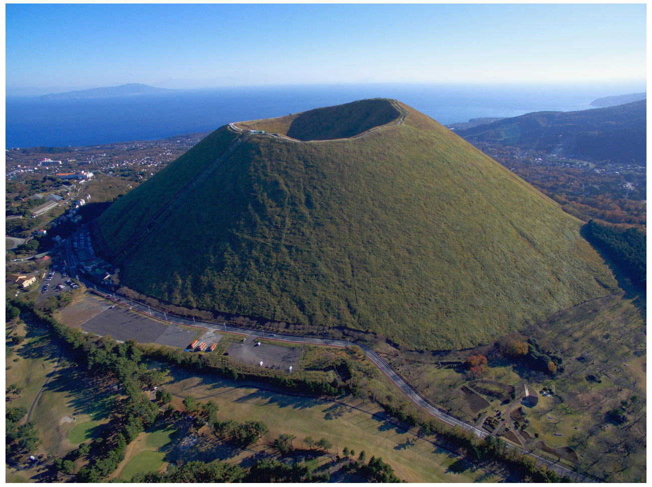
Figure 1 Photograph of the Izu–Omuroyama scoria cone from the northwest, taken by an unmanned aerial vehicle (Koyama, 2017).

The bulk density of typical continental crust is about 2.6–2.7×10³ kg m⁻³. The bulk densities reported for scoria deposits are 0.84–1.01×10³ kg m⁻³ (Taha and Mohamed, 2013) and 0.56–1.20×10³ kg m⁻³ (Bush, 2001). Therefore, the maximum expected density contrast is about 1.4–2.0×10³ kg m⁻³, due to the difference in porosity between welded rocks and scoria deposits. In addition, the Izu–Omuroyama scoria cone is an ideal target for multi-directional muography due to the accessibility of detector sites and absence of muographic shadows from any direction caused by other topographic features.

3 Multi-directional muography observations using emulsion cloud chambers

3.1 Detector design

Emulsion films were manufactured by pouring 70 µm of nuclear emulsion on both sides of a 180 µm thick plastic base. The size of a film is 125 × 100 mm. The films were vacuum-packed in a light-blocking envelope to maintain their planar form, which prevented air bubbles from forming between the envelope and film, and made it easy to handle the films in the field.

The detector used for the 2018 observations is basically the same as that of Nishiyama et al. (2014), and only the number of lead plates was different. The former consists of 20 films and 9 plates of 1 mm thick lead, the latter consists of 20 films and 19 lead plates. At the time of installation in 2018, the films, lead plates, and supports were all in pieces and, therefore, much time and effort was required for assembly in the field. A more efficient detector design was required for rapid and error-free installation.

The detector used in the 2019 observations was improved. It consists of an ECC and an outer box. The ECC consists of 20 emulsion films and 19 lead plates, each 1 mm thick (Fig. 2a). An aluminum frame was fixed to a lead plate with a thin sheet of glue, and then an emulsion film with the light-blocking envelope was attached with scotch tape. In this paper, we term this unit the emulsion–lead plate (EL plate; Fig. 2a). The EL plate was designed for quick assembly in the field.

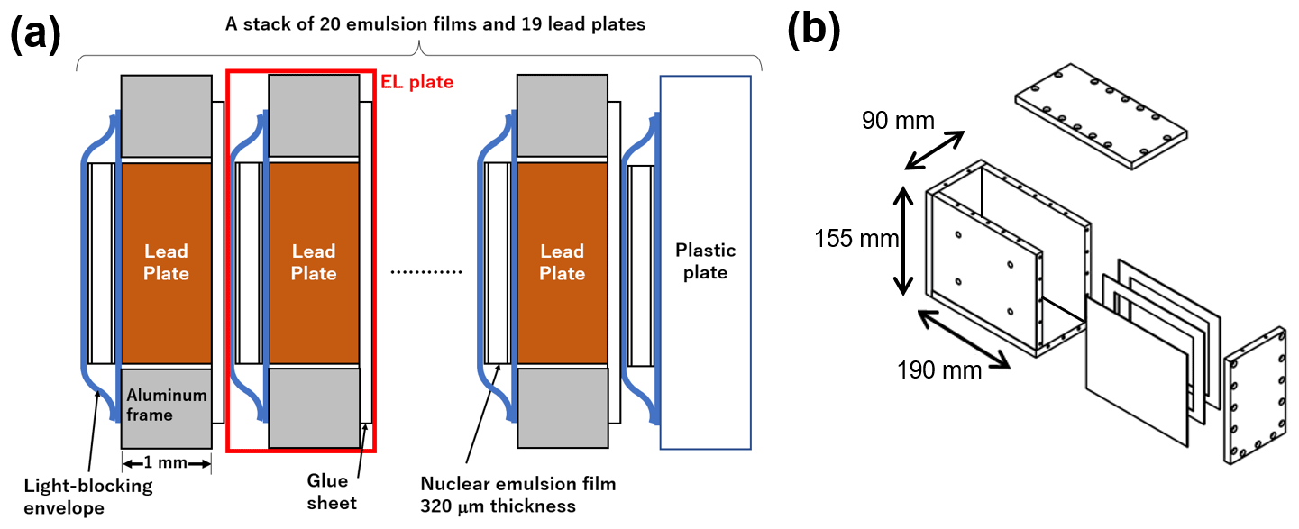
Figure 2 Design of the ECC and outer box. (a) Schematic cross-section of the EL plates and an ECC. The EL plates consist of a 1 mm thick aluminum frame, 1 mm thick lead plate, 100 µm thick glue sheet that fixes a lead plate to an aluminum frame, and an emulsion film with a light-blocking envelope. An ECC consists of 19 EL plates and an emulsion film with a plastic plate. (b) Schematic of the aluminum outer box. The thickness of the aluminum plate is 10 mm. The ECC shown in (a) was set inside this box. There are four holes for feed screws in the front plate.

The outer box consists of 10 mm thick aluminum plates (Fig. 2b). The outer size of this box is 190 mm in width, 155 mm in height, and 90 mm in depth. An ECC and strong springs were placed in the box. There are four screw holes on one side of the box, and by turning the bolts and pushing the spring plate, a uniform pressure (∼ 10⁵ Pa) was applied to the ECC. This pressure prevents the film from stretching and shrinking due to temperature changes.

Given that there is no temporal resolution in emulsion films, ordinary ECC detectors cannot distinguish whether cosmic ray tracks pass the ECC during muographic observation or during transportation and standby. Thus, we also added a similar feature to previous muographic studies using emulsion films. Researchers have used emulsion films with a different alignment during muon observation and during standby (e.g., Tanaka et al., 2007). In the present study, the corners of the EL plates were aligned during the muon observations, while the corners were intentionally shifted a few millimeters horizontally and fixed with clamps during standby (Fig. 3). This alignment difference distinguishes passing charged particles during non-observation and observation periods by pattern matching each emulsion film. By using this procedure, the time to set the alignment between each EL plate in the field is <30 s. Although the muon tracks that pass through an ECC during the alignment set-up may become noise, our procedure reduced such tracks.

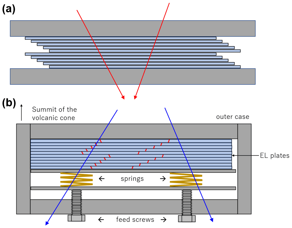
Figure 3 (a) View of the EL plates from above during standby. The EL plates were intentionally shifted a few millimeters horizontally and fixed with a pair of steel plates and a clamp. The red lines represent the muon tracks in this alignment. (b) View from above during the observations. The EL plates were aligned to the side of the outer box, and fixed by the springs and feed screws. The blue lines represent muon tracks during observations. Note that the red tracks cannot be reconstructed in this alignment.

3.2 Installation

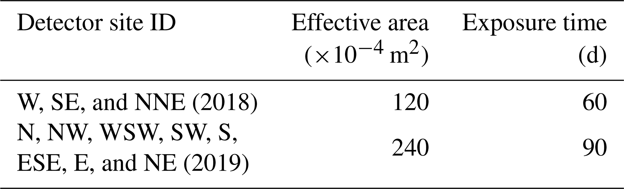
The detectors were installed at three sites in 2018 and eight sites in 2019 around the Izu–Omuroyama scoria cone (Fig. 4; Table 1). Each detector was buried in a hole that was about 40 cm deep to avoid high temperatures due to direct sunlight. This is done because the number of latent image specks decreases and the number of randomly generated specks increases under high-temperature conditions (Nishio et al., 2020).

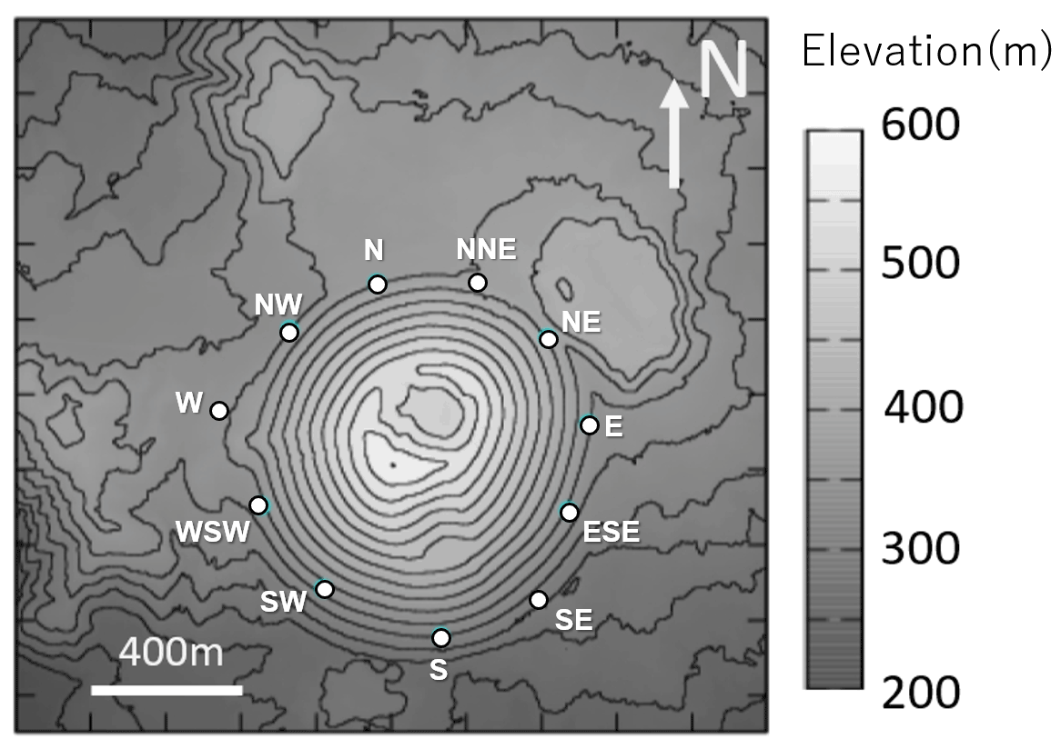
Figure 4 Topography of the Izu–Omuroyama scoria cone. White dots represent observation sites.

Table 1 Effective area and muon exposure time for each detector.

The installation procedure at each observation site in 2019 was as follows (Fig. 5).

1. Carry the outer box and EL plates to the observation site.

2. Measure the coordinates of the site with a hand-held GPS (Garmin; model GPS eTrex 30J). The typical uncertainty of the latitudinal and longitudinal coordinates is 3 m.

3. Dig a hole in the ground with horizontal dimensions of 60 × 40 cm and a depth of 40 cm.

4. Flatten the base of the hole, place a plastic bag inside the hole, and lay down a piece of plywood.

5. Put double-sided tape on the bottom of the outer box and place it on the plywood.

6. Put the stack of EL plates into the box and quickly align them (<30 s).

7. Close the cap of the outer box.

8. Turn the feed screws to increase the pressure.

9. Measure the attitude of the outer box (i.e., the yaw, that is, absolute azimuth angle; roll; and pitch). The yaw is measured with a fiber optic gyro (Japan Aviation Electronics Industry Ltd.; model FOG JM7711; Watanabe et al., 2000), and the roll and pitch are measured by the digital leveler. The typical errors in the yaw, roll, and pitch are $\mathrm{8.7}\times {\mathrm{10}}^{-\mathrm{3}}$, $\mathrm{1.0}\times {\mathrm{10}}^{-\mathrm{3}}$, and $\mathrm{1.0}\times {\mathrm{10}}^{-\mathrm{3}}$ radians, respectively.

10. Cover with styrofoam to avoid heating from the ground surface.

11. Close the plastic bag to keep water out.

12. Backfill the hole.

The time taken for this installation was ∼ 2 h for each site, and we installed detectors as three sites in a day in 2019. The detector retrieval procedure was the opposite of the installation procedure. The 380 films were developed in a darkroom. The deposited silver particles on the surface of the films were removed with anhydrous ethanol. The gelatin of the sensitive layer was swollen with a glycerin solution to obtain the optimum thickness for an automated track readout system, which is described in the next section.

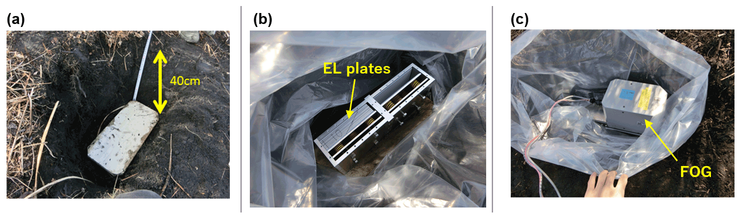
Figure 5 Photographs showing the installation procedure. (a) Dig a hole and place a plywood sheet in the bottom. (b) Place the outer box in the hole and put a stack of EL plates into the box. The plates were aligned over a period of <30 s. After closing the top plate of the box, the feed screws were tightened to increase the pressure. (c) The yaw, roll, and pitch were measured with a fiber optic gyro (FOG) and digital leveler.

4 Track reconstruction, selection, and detection efficiency estimation

4.1 Track reconstruction

A track of a high-energy charged particle is recorded as an aligned line of silver grains in the emulsion film (e.g., Nakamura et al., 2005). The images in the 380 nuclear emulsion films were scanned and the positions and slopes of the tracks were digitized by the “HTS”, a high-speed automated track readout system at Nagoya University (Yoshimoto et al., 2017). For each ECC, the tracks of the charged particles were digitally reconstructed from the segmented tracks in 20 films. NETSCAN 2.0 software was used for track reconstruction (Hamada et al., 2012). NETSCAN 2.0 rapidly corrects for film distortions and local misalignments between films by using many tracks recorded over a large area. It then outputs all possible connections as the final result. NETSCAN 2.0 has been used in various fields, such as neutrino physics (Hiramoto et al., 2020), cosmic ray astronomy (Takahashi et al., 2015), and muographic studies of Egyptian pyramids (Morishima et al., 2017). The typical procedure for the track reconstruction is as follows.

1. Reconstruct the “base track”, which is connected between the emulsion layers across the plastic base of 170 µm in a film.

2. Reconstruction of the “linklet”, which is the base track pair between adjacent films across lead plates.

3. Reconstruction of the tracks that connect across the whole ECC. If no base track was found in two consecutive films on the extension of a track, then the track was considered to have stopped.

For example, in ECC_ID = 02, 8.9 × 10⁶ base tracks, 3.2 × 10⁶ linklets in a pair of adjacent films, and 1.7 × 10⁷ tracks in an entire ECC were reconstructed.

4.2 Track selection

NETSCAN 2.0 outputs all possible track connections. Therefore, it is necessary to carefully select the tracks for the muographic analysis. A schematic example of the output tracks is shown in Fig. 6. Most of the branches can be considered to represent contamination by fake base tracks caused by random noise, or the coincidental occurrence of low-energy positrons/electrons on parallel slopes in the vicinity of the real tracks (e.g., Fig. 6; cases 2 and 3). For reference, the position dependence of noise density is described in Appendix A. Some branches consist of a pair of straight tracks with small closest distances and similar angles (Fig. 6; case 4). In this case, the two tracks should be separated.

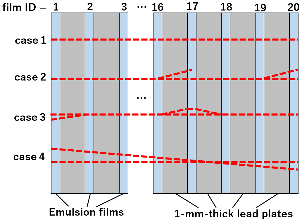
Figure 6 Schematic examples of typical reconstructed tracks in an ECC obtained by NETSCAN 2.0. Upstream means towards the volcanic cone side and downstream means the backward free sky direction. Case 1: a straight track without any branches. Case 2: a straight track with a branch in the middle and downstream films. The track branch in the middle was rejected by selection step 1. The branch in the most downstream film was merged into the straight track by selection step 3a. Case 3: branches in the upstream and middle films. Both branches were merged into a straight track by selection step 3a. Case 4: a pair of straight tracks with small closest distances and similar angles. If the shared proportion of the track length was <20 %, the tracks were divided into two different tracks by selection step 3b.

The following ${\mathit{\chi }}^{\mathrm{2}}/$ ndf value was calculated for all tracks for the low-momentum cut-off:

$$\begin{array}{}\text{(2)}& {\mathit{\chi }}^{\mathrm{2}}/\mathrm{ndf}=\sum _m\left[{\left({\displaystyle \frac{\mathrm{\Delta }{\mathit{\theta }}_R^m}{{\mathit{\sigma }}_R^m}}\right)}^{\mathrm{2}}+{\left({\displaystyle \frac{\mathrm{\Delta }{\mathit{\theta }}_L^m}{{\mathit{\sigma }}_L^m}}\right)}^{\mathrm{2}}\right]/\mathrm{ndf},\end{array}$$

where ndf is the number of degrees of freedom and m is the index of adjacent film pairs (i.e., [1,2], [2,3], [3,4], …, and [18,19], [19,20] in Fig. 6) or with one skip if there was a base track inefficiency (i.e., [1,3], [2,4], [3,5], …, [17,19], [18,20]). $\mathrm{\Delta }{\mathit{\theta }}_R^m=(\mathrm{\Delta }{\mathit{\theta }}_x^m\times \tan {\mathit{\theta }}_x+\mathrm{\Delta }{\mathit{\theta }}_y^m\times \tan {\mathit{\theta }}_y)/\sqrt{{\tan }^{\mathrm{2}}{\mathit{\theta }}_x+{\tan }^{\mathrm{2}}{\mathit{\theta }}_y}$ and $\mathrm{\Delta }{\mathit{\theta }}_L^m=(\mathrm{\Delta }{\mathit{\theta }}_y^m\times \tan {\mathit{\theta }}_x-\mathrm{\Delta }{\mathit{\theta }}_x^m\times \tan {\mathit{\theta }}_y)/\sqrt{{\tan }^{\mathrm{2}}{\mathit{\theta }}_x+{\tan }^{\mathrm{2}}{\mathit{\theta }}_y}$, and $\mathrm{\Delta }{\mathit{\theta }}_x^m$ and $\mathrm{\Delta }{\mathit{\theta }}_y^m$ are angular differences along the x, y coordinates of the ECC. ${\mathit{\sigma }}_R^m$ and ${\mathit{\sigma }}_L^m$ are the root mean square of $\mathrm{\Delta }{\mathit{\theta }}_R^m$ and $\mathrm{\Delta }{\mathit{\theta }}_L^m$, calculated for every adjacent film pair in every ECC (Fig. 7). Figure 8 shows the distribution of ${\mathit{\chi }}^{\mathrm{2}}/$ ndf for all tracks in an ECC.

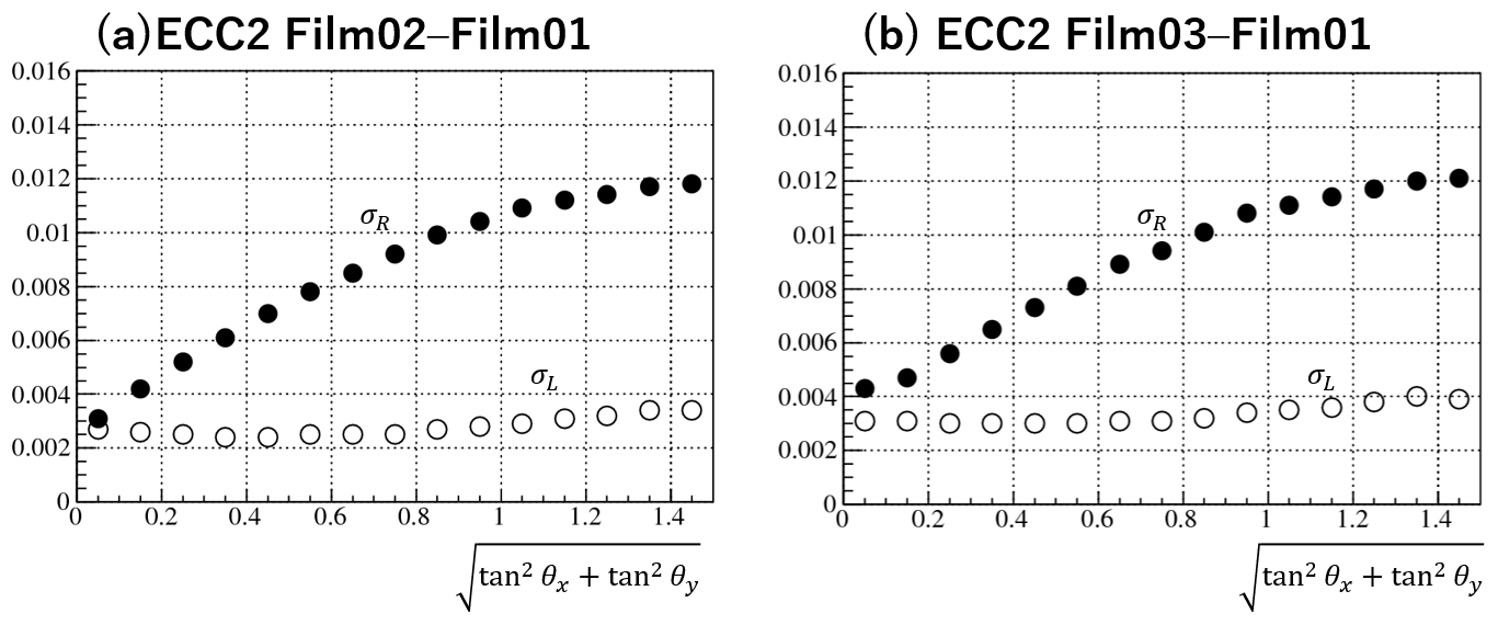
Figure 7 Examples of σ_R and σ_L as a function of $\sqrt{{\tan }^{\mathrm{2}}{\mathit{\theta }}_x+{\tan }^{\mathrm{2}}{\mathit{\theta }}_y}$. The values were determined by the ECC and used to calculate the value of Eq. (2).

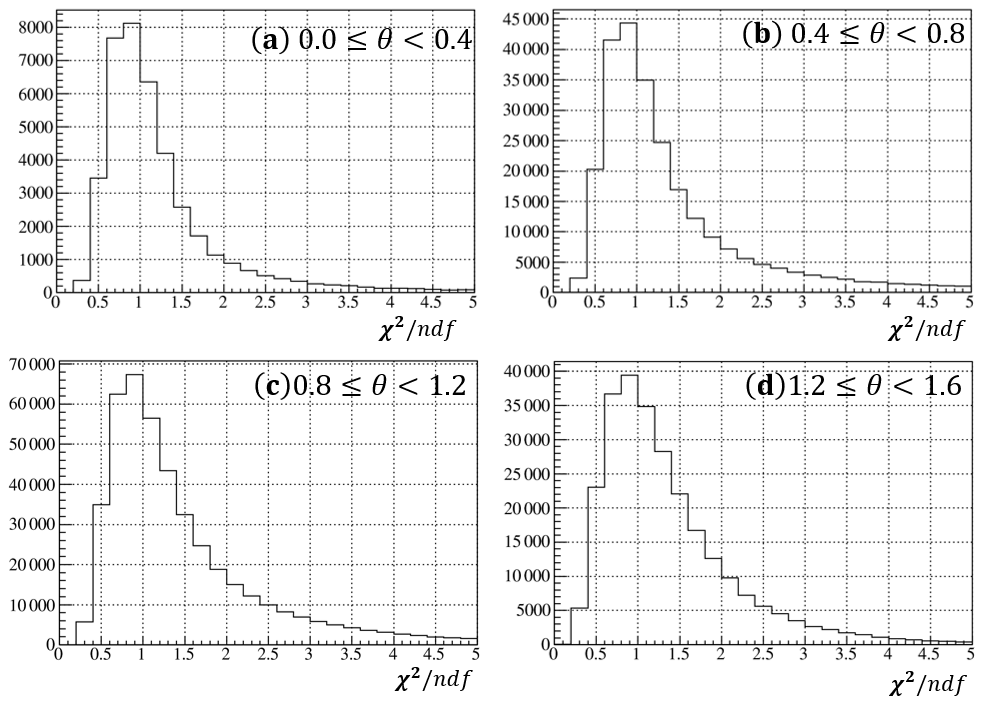
Figure 8 Example of the ${\mathit{\chi }}^{\mathrm{2}}/$ ndf distribution for selected tracks as a function of $\mathit{\theta }=\sqrt{{\tan }^{\mathrm{2}}{\mathit{\theta }}_x+{\tan }^{\mathrm{2}}{\mathit{\theta }}_y}$ in an ECC. (a) $\mathrm{0}\le \mathit{\theta }<\mathrm{0.4}$, (b) $\mathrm{0.4}\le \mathit{\theta }<\mathrm{0.8}$, (c) $\mathrm{0.8}\le \mathit{\theta }<\mathrm{1.2}$, and (d) $\mathrm{1.2}\le \mathit{\theta }<\mathrm{1.6}$.

The procedure for track selection is as follows.

• 1.

  Select tracks that start from one of the two most upstream (i.e., summit cone side) films and stop at one of the two most downstream films.

• 2.

  Select tracks with ${\mathit{\chi }}^{\mathrm{2}}/\mathrm{ndf}<\mathrm{5.0}$.

• 3.

  If a track has any branches, then do the following:

  • a.

    If the shared proportion of track length is ≥ 20 %, choose the longest branch. If the track lengths are the same, then choose the branch with the smallest ${\mathit{\chi }}^{\mathrm{2}}/$ ndf.

  • b.

    If the shared proportion of track length is <20 % (Fig. 6; case 4), then divide the branches into two tracks.

We estimated the effect of the straightness filtering using ${\mathit{\chi }}^{\mathrm{2}}/\mathrm{ndf}<\mathrm{5.0}$. Figure 9 shows the momentum filtering efficiency. This figure was derived from a simple simulation in which the interaction of charged particles inside the ECC was assumed to be multiple Coulomb scattering only, and the scattering angle was approximated by a Gaussian distribution. The path length in the lead plates (i.e., x in Eq. 1) becomes longer when the track has a larger slope, and thus the maximum detectable momentum (i.e., p_max in Eq. 1) also becomes higher. Based on the background noise study by Nishiyama et al. (2016), the size of the mountain body used in the simulation and the Izu–Omuroyama scoria cone is broadly the same, and thus the rejection efficiency should be sufficient. For example, after the track selection, 1.7 × 10⁶ tracks were selected at the site N.

Figure 9 Survival ratio of muons after the straightness cut-off as a function of momentum. (a) Track angles with tan (relative azimuth)=0.0 and tan (elevation angle)=0.0. (b) Track angles with tan (relative azimuth)=1.0 and tan (elevation angle)=1.0. The path length in the lead plates becomes longer when the track has a larger slope, and thus the remaining momentum also becomes higher for the latter case. The momentum values at a survival ratio of 0.5 are 0.6 and 1.1 GeV $/$ c, respectively.

4.3 Detection efficiency estimation

The muon detection efficiency can be estimated by investigating the percentage of tracks that have a base track in a film. In this paper, we term this percentage the “fill factor”. The fill factor ε can be defined as follows:

$$\begin{array}{}\text{(3)}& {\mathit{\epsilon }}_j\left({\mathit{\theta }}_x,{\mathit{\theta }}_y\right)={\displaystyle \frac{N_j\left({\mathit{\theta }}_x,{\mathit{\theta }}_y\right)}{N_{j-\mathrm{1},j+\mathrm{1}}\left({\mathit{\theta }}_x,{\mathit{\theta }}_y\right)}},\end{array}$$

where j is a film ID, $N_{j-\mathrm{1},j+\mathrm{1}}\left({\mathit{\theta }}_x,{\mathit{\theta }}_y\right)$ is the number of tracks in which base tracks were found in films j−1 and j+1, and N_j(θ_x, θ_y) is the number of tracks in which base tracks were found in films j−1, j, and j+1. The fill factor depends on the films and track slopes θ_x and θ_y. The position dependence of the fill factor is described in Appendix A.

Using the fill factor ε_j(θ_x,θ_y) and ${\stackrel{\mathrm{‾}}{\mathit{\epsilon }}}_j\left({\mathit{\theta }}_x,{\mathit{\theta }}_y\right)=\mathrm{1}-{\mathit{\epsilon }}_j\left({\mathit{\theta }}_x,{\mathit{\theta }}_y\right)$, the muon detection efficiency ϵ in an ECC can be calculated as follows:

$$\begin{array}{}\text{(4)}& \mathit{ϵ}\left({\mathit{\theta }}_x,{\mathit{\theta }}_y\right)=\sum _{\mathrm{hit}\mathrm{pattern}}{\mathit{\epsilon }}_{\mathrm{1}}\times {\stackrel{\mathrm{‾}}{\mathit{\epsilon }}}_{\mathrm{2}}\times {\mathit{\epsilon }}_{\mathrm{3}}\times \mathrm{\dots }\times {\stackrel{\mathrm{‾}}{\mathit{\epsilon }}}_{\mathrm{18}}\times {\mathit{\epsilon }}_{\mathrm{19}}\times {\mathit{\epsilon }}_{\mathrm{20}},\end{array}$$

where “hit pattern” is the summation for all possible hit patterns (e.g., ${\mathit{\epsilon }}_{\mathrm{1}}\times {\stackrel{\mathrm{‾}}{\mathit{\epsilon }}}_{\mathrm{2}}\times {\mathit{\epsilon }}_{\mathrm{3}}\times \mathrm{\dots }\times {\stackrel{\mathrm{‾}}{\mathit{\epsilon }}}_{\mathrm{18}}\times {\mathit{\epsilon }}_{\mathrm{19}}\times {\mathit{\epsilon }}_{\mathrm{20}}$ or ${\stackrel{\mathrm{‾}}{\mathit{\epsilon }}}_{\mathrm{1}}\times {\mathit{\epsilon }}_{\mathrm{2}}\times {\mathit{\epsilon }}_{\mathrm{3}}\times \mathrm{\dots }\times {\mathit{\epsilon }}_{\mathrm{18}}\times {\stackrel{\mathrm{‾}}{\mathit{\epsilon }}}_{\mathrm{19}}\times {\mathit{\epsilon }}_{\mathrm{20}})$ from the track selection conditions described in section 4.2 (Fig. 10). An example of the angular distribution of the fill factor ε_j(θ_x, θ_y) and muon detection efficiency ϵ(θ_x, θ_y) in an ECC is shown in Fig. 11. The statistics of observed muons were limited in some angular bins by the thick volcanic cone. However, the statistics were sufficient in the backward region (i.e., elevation angle <0.0). We used the distribution of the negative elevation angular region instead of the positive region, because it has enough statistics and the optics of the HTS has an approximately two-fold rotational symmetry.

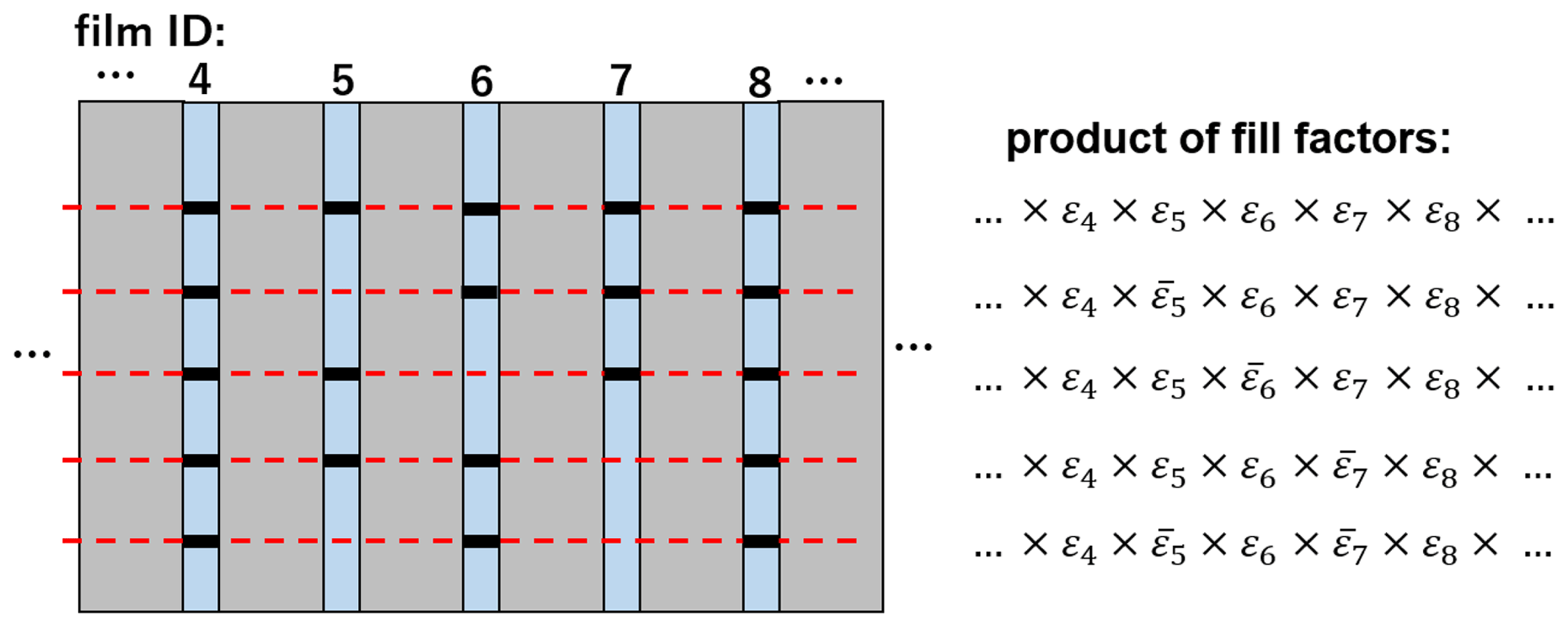
Figure 10 Example of all hit patterns and the products of fill factors in Eq. (4) when base tracks are found in film ID numbers 4 and 8. The red lines indicate the reconstructed tracks and the short black lines represent the base tracks found in the films.

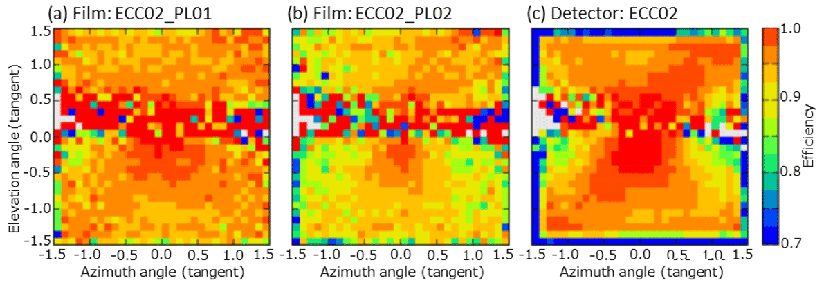
Figure 11 Examples of the angular distribution of the fill factor in some films and the efficiency of an ECC. (a) Fill factor for film ID = PL01 (most upstream film) and ECC ID = 02 at site N. (b) Fill factor for film ID = PL02 and ECC ID = 02. (c) Muon detection efficiency for ECC ID = 02 as evaluated by Eq. (4). The horizontal axis is the tangent of the azimuth angle; the vertical axis is the tangent of the elevation angle; the colors represent the fill factor/efficiency values. A positive elevation angle means the muon path is from the cone; a negative elevation angle means the muon path is from the backward free sky. The gray color means there were no observed muons in the angular bin due to the thick volcanic cone.

5 Results

The average density along muon path was determined for each observation site. We used the muon flux model of Honda et al. (2004), energy loss model of Groom et al. (2001), and topography around the Izu–Omuroyama scoria cone from the Geospatial Information Authority of Japan (https://maps.gsi.go.jp/, last access: 11 March 2022). The coordinates of the observation site, direction, sensitive area, thickness of the ECC detectors, and observation time were used to calculate the expected number of muons at each observation site. The expected number of muons can be calculated as a function of the average density ρ_k along the path:

$$\begin{array}{}\text{(5)}& N_k^{\mathrm{simu}}\left({\mathit{\rho }}_k\right)=f_k\left({\mathit{\rho }}_k{L}_k\right)\times S_k\times {\mathrm{\Omega }}_k\times T\times {\mathit{ϵ}}_k,\end{array}$$

where k is the index of an angular bin, f_k(ρ_kL_k) is the penetrating muon flux (calculated from the muon flux model, energy loss model, and path length L_k), S_k is the sensitive area of the ECC, Ω_k is the solid angle, ϵ_k is the muon detection efficiency, and T is the observation time.

The angular bin size used for calculating the expected value was (0.01)² in terms of the tangent. The angular bins were then merged to improve the statistical accuracy of the observed values. This merging procedure is useful in topology where a small change in elevation angle can dramatically change the path length in the volcano. If k is the index of the angular bins of (0.01)² and the bins belong to a larger angular bin i, then the following equation holds:

$$\begin{array}{}\text{(6)}& N_i^{\mathrm{merged}}\left({\mathit{\rho }}_i\right)=\sum _k{N}_k^{\mathrm{simu}}\left({\mathit{\rho }}_i\right),\end{array}$$

where ρ_i is the density of the merged angular bin i. If $N_i^{\mathrm{obs}}$ is the number of the detected muons in the angular bin i, then we can uniquely determine the density value ρ_i, such that $N_i^{\mathrm{merged}}\left({\mathit{\rho }}_i\right)=N_i^{\mathrm{obs}}$. The lower limit ${\mathit{\rho }}_i^{\mathrm{low}}$ and upper limit ${\mathit{\rho }}_i^{\mathrm{up}}$ caused by the statistical error in $N_i^{\mathrm{obs}}$ can also be estimated as follows:

$$\begin{array}{}\text{(7)}& {\displaystyle }{N}_i^{\mathrm{merged}}\left({\mathit{\rho }}_i^{\mathrm{low}}\right)=N_i^{\mathrm{obs}}+\sqrt{N_i^{\mathrm{obs}}},\text{(8)}& {\displaystyle }{N}_i^{\mathrm{merged}}\left({\mathit{\rho }}_i^{\mathrm{up}}\right)=N_i^{\mathrm{obs}}-\sqrt{N_i^{\mathrm{obs}}}.\end{array}$$

An example of the derived density map is shown in Fig. 12. All results are shown in Figs. B1–B10 (Appendix B).

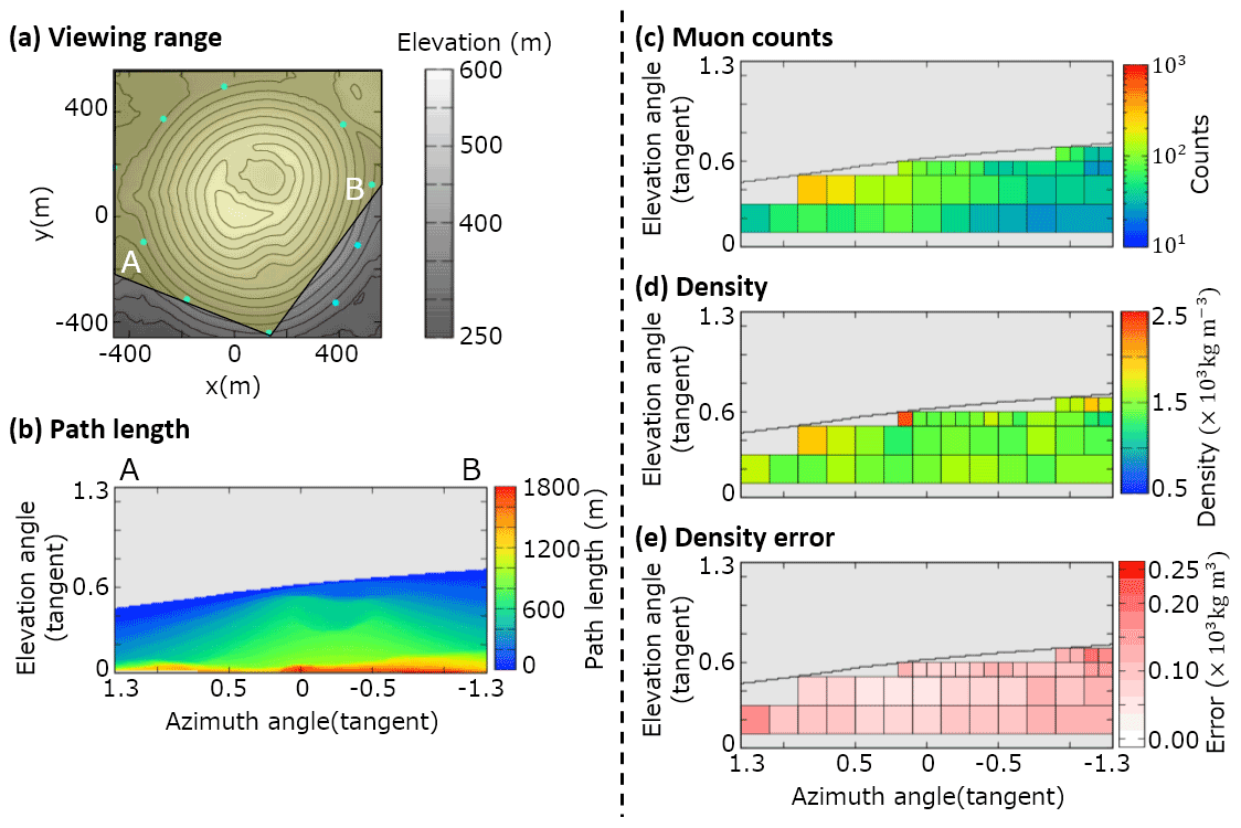
Figure 12 Data for observation site N. (a) Map, topography, and viewing range; (b) path length of the volcanic cone; (c) muon counts $N_i^{\mathrm{obs}}$; (d) density ρ_i. The maximum value of the color bar indicates a density of >2.5×10³ kg m⁻³ and the minimum value is <0.5×10³ kg m⁻³. (e) Density error $\mathrm{\Delta }\mathit{\rho }=\left({\mathit{\rho }}_i^{\mathrm{up}}-{\mathit{\rho }}_i^{\mathrm{low}}\right)/\mathrm{2}$. The maximum value of the color bar indicates a density error of >0.25×10³ kg m⁻³.

The definition of the angular bin areas was based on the following. The size of the angular bins was (0.2)² when the elevation angle was 0.1 to 0.5 in tangent terms. When the elevation angle was >0.5, the angular bin size was (0.1)². If the observed muon count in the bin was <25, the angular bin was manually merged with adjacent bins to improve the statistical error. The angular bin with a near-surface path (path length < 30 m) was excluded to avoid ambiguity between the actual topography and digital elevation map. The attitude errors of each muon detector also contribute to the path length ambiguity, especially near the surface of the cone.

6 Validation

Firstly, we validated the observed muon flux by comparing it with the muon flux model in the free sky region. The average and standard deviation of the ratio between the sites were 88 % ± 4 % in the forward direction and 92 % ± 2 % in the backward direction, except for the NNE site (Fig. 13). An example of observed/expected muon flux ratio angular distribution of the site N is shown in Fig. 14. As can be seen in this figure, in each detector site, a non-uniform distribution of the observed/expected muon flux ratio exists. Such deviations were 4 %–7 % except for the forward directions at the sites SE and NNE. For reference, a 10 % error in the flux corresponds to a 4 % error in the density length at a tan(elevation angle) = 0.2 and density length = 1000 m (water equivalent). These deviations were less than the errors caused by the muon statistics. The discrepancy for the NNE site is discusses in the next section.

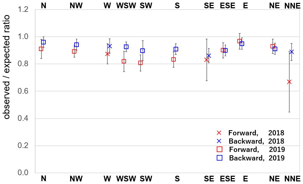
Figure 13 The observed $/$ expected muon flux ratio for each observation site in the free sky region. The plot represents the average value of the ratio in tangential angular space, and the error bars are the standard deviations at each site.

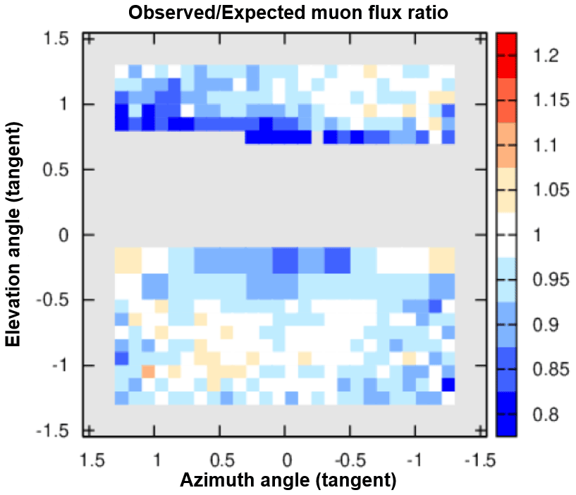
Figure 14 Example of the observed $/$ expected muon flux ratio in the free sky region at site N. The horizontal axis represents the azimuth angle, and the vertical axis represents the elevation angle. Positive elevation angle means the muons come from forward directions (the volcanic cone). Negative elevation angle means the muons come from backward free sky directions. The typical deviation of the ratio is 4 %–7 % in each site.

Secondly, we compared the density of the entire volcanic cone determined by gravity data with that obtained by muography. Table 2 shows the density determined from each observation site when the cone is assumed to be uniform. The calculation of the overall density $\stackrel{\mathrm{‾}}{\mathit{\rho }}$ is as follows:

$$\begin{array}{}\text{(9)}& \stackrel{\mathrm{‾}}{\mathit{\rho }}={\displaystyle \frac{{\sum }_i{\mathit{\rho }}_i{V}_i}{{\sum }_i{V}_i}},\end{array}$$

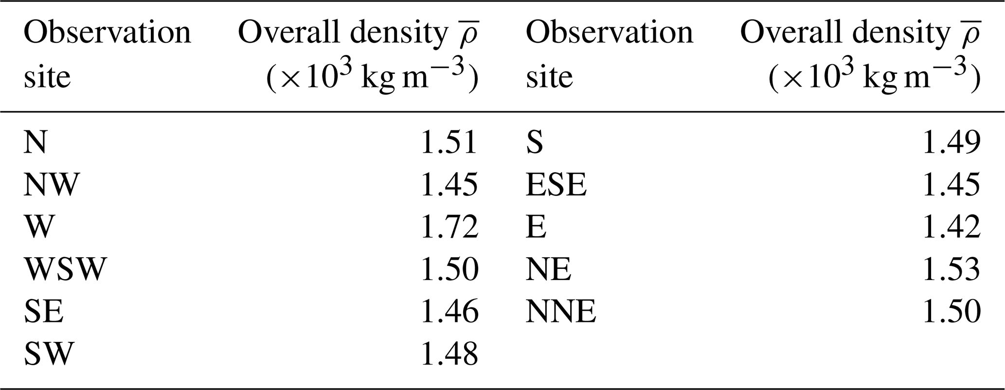
where i is the index of the angular bins and V_i is the volume of the volcanic cone cut off by the angle bin i. Based on the gravity study of Nishiyama et al. (2020), the density of the Izu–Omuroyama scoria cone is $\mathrm{1.39}\pm \mathrm{0.07}\times {\mathrm{10}}^{\mathrm{3}}$ kg m⁻³. The overall density derived by muography at each observation site is 1.42–1.53 × 10³ kg m⁻³, except for one site. These values are broadly consistent with the density determined from gravity data, except for the observation site W (1.72 × 10³ kg m⁻³).

Table 2 Overall bulk density obtained by muography, assuming that the density is uniform in the volcanic cone.

7 Discussion

For the observed $/$ expected muon flux ratio in the free sky region, the values in the forward direction are less than in the backward direction at many observation sites. This could be because the detectors were buried in holes on steep slopes (∼ 30^∘), and our analysis might not account for that effect. Due to the steep slope, muons arriving from the forward direction need to penetrate some amount of soil, whereas muons from the backward direction can enter the detector without being affected by the soil cover. In addition, the resolution of the detector coordinates is ∼ 3 m, which might also contribute to the discrepancy.

Some density results from near the ground surface are complex. Some regions near the path length of 30 m appear to have relatively higher or lower density than the other data (e.g., Figs. B6, B9). One possible reason for this is the error in the detector attitude. Near the surface of the volcanic cone, the difference between the calculated and actual path lengths may become larger due to the error in the detector attitude.

The anomalous data for the NNE site also warrants further consideration. The reason for this might be a difference between the digital elevation map and actual topography. There is a stone wall in front of the buried detector at this site, which is about 1 m high and located on the volcanic cone side. The grid size of the digital elevation map used in this study is 1 m, and thus the map might not record this steep gradient.

In summary, errors in the position and attitude of the detectors, and the accuracy of the DEM, might cause a misfit between the DEM and actual topography. These are the main reasons for the discrepancy between the observed and expected muon flux.

The discrepancy between the observed and expected muon flux was ±4 % in the forward direction and ±2 % in the backward direction between the detectors. In addition, the typical deviation inside each site was 4 %–7 %. These values are smaller than the statistical error of the observed muons used to determine the density of the volcanic cone, and thus they were not significant for our observations. It is interesting to consider if an improvement in the accuracy of the detector position and attitude, and the DEM, would decrease this systematic error. For example, the ±4 % deviation in the forward direction would be expected to decrease to ±2 %, because the misfit effect is less in the backward direction. Further improvements will require simulation of the expected muon flux that take into account more processes and verification of the systematic errors associated with the ECC detectors.

The obtained density values (1.42–1.53×10³ kg m⁻³; this study) and $\mathrm{1.39}\pm \mathrm{0.07}\times {\mathrm{10}}^{\mathrm{3}}$ kg m⁻³ (Nishiyama et al., 2020) for the Izu–Omuroyama scoria cone are broadly consistent (Table 2). In a study by Rosas-Carbajal et al. (2017), the density value obtained from gravity data was 0.5 × 10³ kg m⁻³ larger the value obtained by muography. In our validation, this discrepancy does not exist. As Rosas-Carbajal et al. (2017) suggested, the discrepancy might be due to differences in the filtering performance for low-momentum particles, as shown in Fig. 9.

The higher density obtained at site W cannot be explained by the systematic errors described above. One possible reason for this is an actual high-density structure in front of the site. This hypothesis is consistent with the fact that lava flowed out from the crater lake to the west (Koyano et al., 1996).

8 Conclusions

A muographic study of the Izu–Omuroyama scoria cone was undertaken in 11 directions. The ECC detector design was optimized for quick installation in the field. We mounted the 11 detectors beneath the ground, surrounding the volcanic cone. The tracks of charged particles that passed through the ECCs were reconstructed using the automated emulsion track readout system HTS and NETSCAN 2.0 software. After track selection, including momentum filtering and efficiency estimation, the density profiles in 2D angular space were derived for each observation site. The methods described in this paper can be applied to the observation of other volcanoes and target objects.

We compared the observed muon flux to the expected value from a muon flux model in the free sky region. The muon flux difference between each detector was 4 % in the forward directions and 2 % in the backward directions, and the typical deviations in each site were about 4 %–7 %. The errors in the detector coordinates and attitude, and DEM, are the main cause of the discrepancy between the observed and expected muon flux.

In addition, we also compared our results with the overall volcanic cone density estimated from gravity data, which are broadly consistent, apart from the W site. This discrepancy for the W site cannot be explained by the systematic errors discussed in the previous section and the statistical error of the observed muons. It might reflect a high-density structure located in the western flank of the volcano. Further 3D density reconstructions of the Izu–Omuroyama scoria cone are ongoing using the data set described in this paper.

Appendix A

We here consider how the position dependency of the detected tracks affects the density results.

The fill factor of the base tracks (i.e., track detection efficiency in a film) also depends on the position of the scanned film. The typical causes of the decrease of the fill factor are heterogeneous thickness of the emulsion layers, some dusts or scratches on the emulsion surface, and the poorly tuned parameters for the scanning.

Figure A1 shows the position distribution of the fill factor of all films of an ECC. For example, on the upper right, the films tend to have a low fill factor (e.g., a–f, h, k, l, q). This part has a larger thickness of the emulsion layer because the drops of the glycerin solution were left in the upper right corner when drying after soaking due to the structure of the developing racks. Figure A1s and t show a larger area of the low fill factor on the right and left. The reason might be the poorly tuned parameters used for the scanning.

Compared to the size of the scoria cone, the ECC is a very small “element”; thus the local position dependence of the fill factor can be approximately treated as an average fill factor ε_j(θ_x,θ_y). The decrease of the fill factor is reflected in ε_j(θ_x,θ_y) in Eq. (4). Finally, ε_j(θ_x,θ_y), which encompasses the effects of the local decrease of the fill factor, is effectively used to derive the angle-dependent muon detection efficiency.

We should also consider the position dependency of noise. Local high density of random silver grains caused by any chemical conditions, or fake images produced by scratches on the films tend to create a group of fake tracks concentrated in one place. In addition, such fake tracks tend to have small slopes by scanning with automated emulsion readout system. If such noise is continuous at the same location on the film, they might make many parallel tracks at a certain slope and give a systematic error in the result. However, such possibility has been eliminated by the track selection algorithm described in the Sect. 4.2, because such concentrated tracks in position and angular space make numerous branches in track connection (see Fig. 6) and tracks with such branches were removed in the selection procedure. Figure A2 shows the number of selected tracks with small slope per mm² in each observation site. The histogram roughly fits the Poisson distribution and there is no remarkable excess. The difference in the peak in the histograms depends on the difference in the exposure time (SE, W, NNE), existence of topography in the backward direction (NE), pitch angle of the detector attitude (e.g., SW has larger pitch angle, thus less tracks of the small slopes from the backward direction), and the difference in muon detection efficiency.

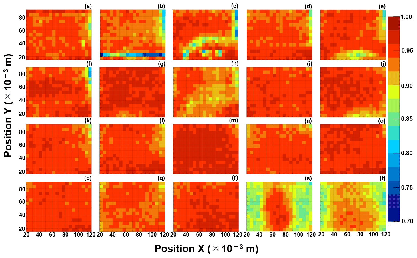
Figure A1 The position distribution of the fill factor in each film of ECC02. (a)–(t) represent PL01–PL20, respectively.

Figure A2 (a) The position distribution of the number of selected tracks per mm² in the ECC02. (b–l) The number of selected tracks per mm² (the black line) with the fitting result of a Poisson distribution ($=\mathit{\alpha }{\mathit{\mu }}^x{e}^{-\mathit{\mu }}/x$, the red line) in each observation site, respectively. The tracks selected for this figure came from in the backward direction and have small slopes ($\left|\tan {\mathit{\theta }}_x\right|<\mathrm{0.5}$ and $\left|\tan {\mathit{\theta }}_y\right|<\mathrm{0.5}$).

Appendix B

The density results for each observation site are shown in Figs. B1–B10.

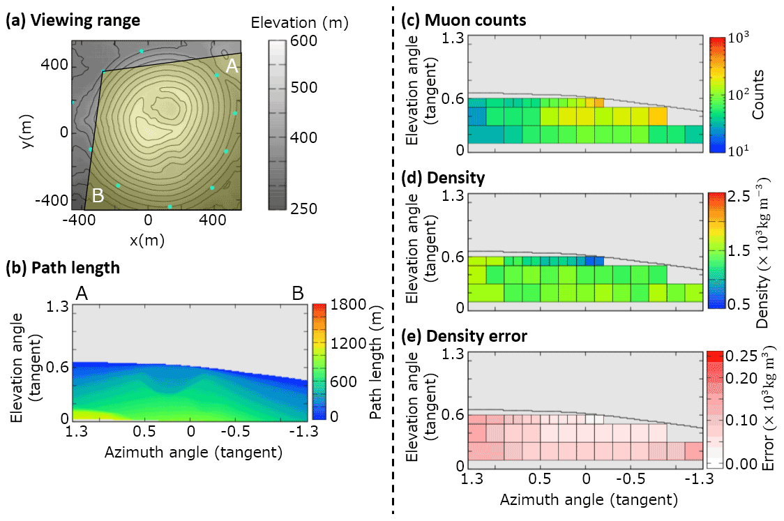
Figure B1 Observation site NW. (a) Map, topography, and viewing range; (b) path length of the volcanic cone; (c) muon counts $N_i^{\mathrm{obs}}$; (d) density ρ_i. The maximum value of the color bar indicates a density of >2.5×10³ kg m⁻³ and the minimum value is <0.5×10³ kg m⁻³. (e) Density error $\mathrm{\Delta }\mathit{\rho }=\left({\mathit{\rho }}_i^{\mathrm{up}}-{\mathit{\rho }}_i^{\mathrm{low}}\right)/\mathrm{2}$. The maximum value of the color bar indicates a density error of >0.25×10³ kg m⁻³.

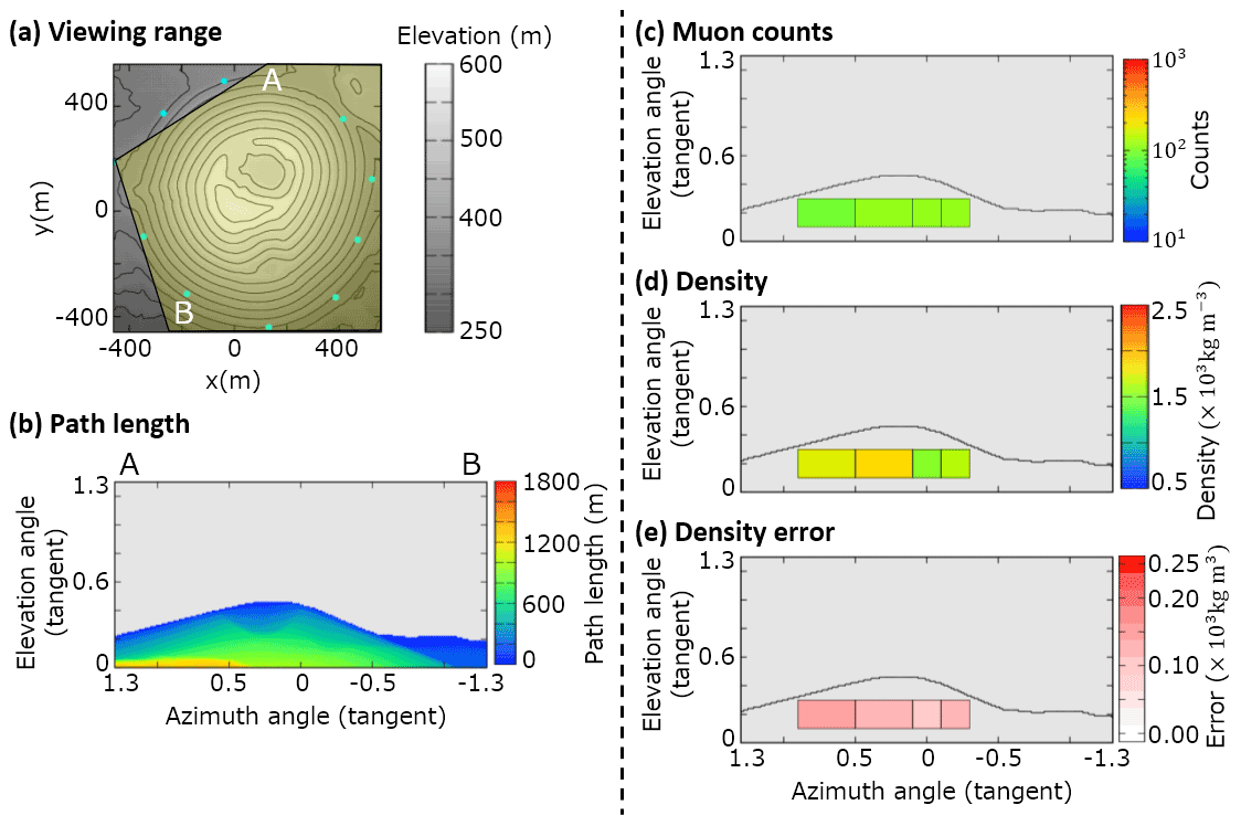
Figure B2 Observation site W. (a) Map, topography, and viewing range; (b) path length of the volcanic cone; (c) muon counts $N_i^{obs}$; (d) density ρ_i. The maximum value of the color bar indicates a density of >2.5×10³ kg m⁻³ and the minimum value is <0.5×10³ kg m⁻³. (e) Density error $\mathrm{\Delta }\mathit{\rho }=\left({\mathit{\rho }}_i^{\mathrm{up}}-{\mathit{\rho }}_i^{\mathrm{low}}\right)/\mathrm{2}$. The maximum value of the color bar indicates a density error of >0.25×10³ kg m⁻³.

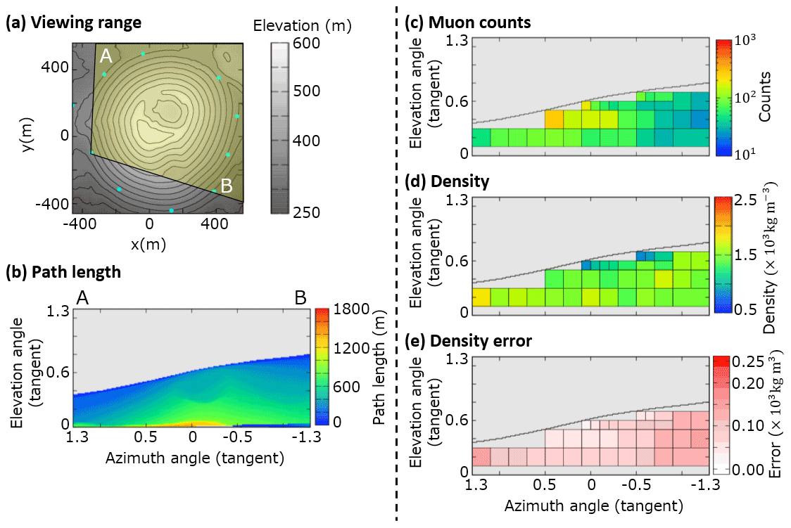
Figure B3 Observation site WSW. (a) Map, topography, and viewing range; (b) path length of the volcanic cone; (c) muon counts $N_i^{\mathrm{obs}}$; (d) density ρ_i. The maximum value of the color bar indicates a density of >2.5×10³ kg m⁻³ and the minimum value is <0.5×10³ kg m⁻³. (e) Density error $\mathrm{\Delta }\mathit{\rho }=\left({\mathit{\rho }}_i^{\mathrm{up}}-{\mathit{\rho }}_i^{\mathrm{low}}\right)/\mathrm{2}$. The maximum value of the color bar indicates a density error of >0.25× 10³ kg m⁻³.

Figure B4 Observation site SW. (a) Map, topography, and viewing range; (b) path length of the volcanic cone; (c) muon counts $N_i^{\mathrm{obs}}$; (d) density ρ_i. The maximum value of the color bar indicates a density of >2.5×10³ kg m⁻³ and the minimum value is <0.5×10³ kg m⁻³. (e) Density error $\mathrm{\Delta }\mathit{\rho }=\left({\mathit{\rho }}_i^{\mathrm{up}}-{\mathit{\rho }}_i^{\mathrm{low}}\right)/\mathrm{2}$. The maximum value of the color bar indicates a density error of >0.25×10³ kg m⁻³.

Figure B5 Observation site S. (a) Map, topography, and viewing range; (b) path length of the volcanic cone; (c) muon counts $N_i^{\mathrm{obs}}$; (d) density ρ_i. The maximum value of the color bar indicates a density of >2.5×10³ kg m⁻³ and the minimum value is <0.5×10³ kg m⁻³. (e) Density error $\mathrm{\Delta }\mathit{\rho }=\left({\mathit{\rho }}_i^{\mathrm{up}}-{\mathit{\rho }}_i^{\mathrm{low}}\right)/\mathrm{2}$. The maximum value of the color bar indicates a density error of >0.25×10³ kg m⁻³.

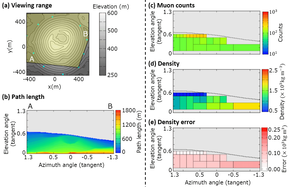
Figure B6 Observation site SE. (a) Map, topography, and viewing range; (b) path length of the volcanic cone; (c) muon counts $N_i^{\mathrm{obs}}$; (d) density ρ_i. The maximum value of the color bar indicates a density of >2.5×10³ kg m⁻³ and the minimum value is <0.5×10³ kg m⁻³. (e) Density error $\mathrm{\Delta }\mathit{\rho }=\left({\mathit{\rho }}_i^{\mathrm{up}}-{\mathit{\rho }}_i^{\mathrm{low}}\right)/\mathrm{2}$. The maximum value of the color bar indicates a density error of >0.25×10³ kg m⁻³.

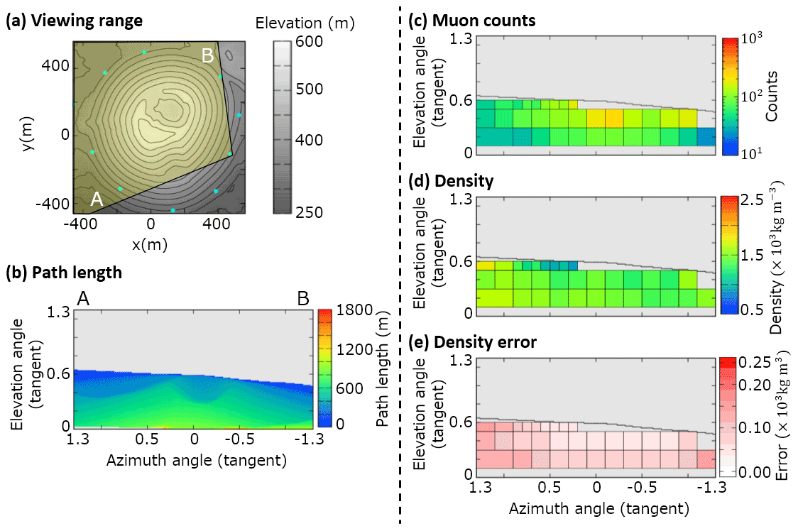
Figure B7 Observation site ESE. (a) Map, topography, and viewing range; (b) path length of the volcanic cone; (c) muon counts $N_i^{\mathrm{obs}}$; (d) density ρ_i. The maximum value of the color bar indicates a density of >2.5×10³ kg m⁻³ and the minimum value is <0.5×10³ kg m⁻³. (e) Density error $\mathrm{\Delta }\mathit{\rho }=\left({\mathit{\rho }}_i^{\mathrm{up}}-{\mathit{\rho }}_i^{\mathrm{low}}\right)/\mathrm{2}$. The maximum value of the color bar indicates a density error of >0.25×10³ kg m⁻³.

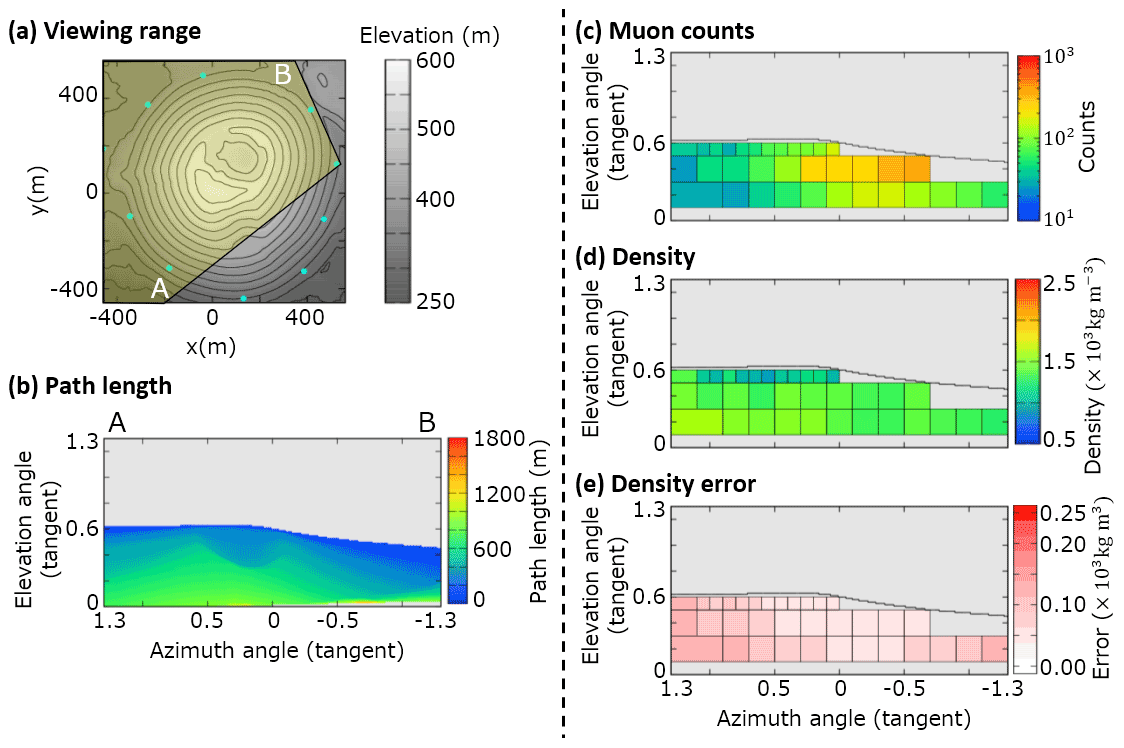
Figure B8 Observation site E. (a) Map, topography, and viewing range; (b) path length of the volcanic cone; (c) muon counts $N_i^{\mathrm{obs}}$; (d) density ρ_i. The maximum value of the color bar indicates a density of >2.5×10³ kg m⁻³ and the minimum value is <0.5×10³ kg ⁻³. (e) Density error $\mathrm{\Delta }\mathit{\rho }=\left({\mathit{\rho }}_i^{\mathrm{up}}-{\mathit{\rho }}_i^{\mathrm{low}}\right)/\mathrm{2}$. The maximum value of the color bar indicates a density error of >0.25×10³ kg m⁻³.

Figure B9 Observation site NE. (a) Map, topography, and viewing range; (b) path length of the volcanic cone; (c) muon counts $N_i^{\mathrm{obs}}$; (d) density ρ_i. The maximum value of the color bar indicates a density of >2.5×10³ kg m⁻³ and the minimum value is <0.5×10³ kg m⁻³. (e) Density error $\mathrm{\Delta }\mathit{\rho }=\left({\mathit{\rho }}_i^{\mathrm{up}}-{\mathit{\rho }}_i^{\mathrm{low}}\right)/\mathrm{2}$. The maximum value of the color bar indicates a density error of >0.25×10³ kg m⁻³.

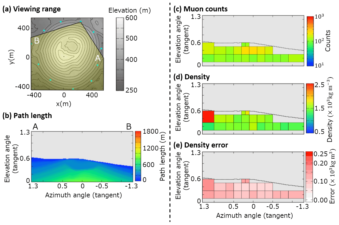
Figure B10 Observation site NNE. (a) Map, topography, and viewing range; (b) path length of the volcanic cone; (c) muon counts $N_i^{\mathrm{obs}}$; (d) density ρ_i. The maximum value of the color bar indicates a density of >2.5×10³ kg m⁻³ and the minimum value is <0.5×10³ kg m⁻³. (e) Density error $\mathrm{\Delta }\mathit{\rho }=\left({\mathit{\rho }}_i^{\mathrm{up}}-{\mathit{\rho }}_i^{\mathrm{low}}\right)/\mathrm{2}$. The maximum value of the color bar indicates a density error of >0.25×10³ kg m⁻³.