On the determination of ionospheric electron density profiles using multi-frequency riometry

Radio wave absorption in the ionosphere is a function of electron density, collision frequency, radio wave polarisation, magnetic field and radio wave frequency. Several studies have used multi-frequency measurements of cosmic radio noise absorption to determine electron density profiles. Using the framework of statistical inverse problems, we investigated if an electron density altitude profile can be determined by using multi-frequency, dual-polarisation measurements. It was found that the altitude profile cannot be uniquely determined from a “complete” measurement of radio wave absorption for all frequencies and two polarisation modes. This implies that accurate electron density profile measurements cannot be ascertained using multi-frequency riometer data alone and that the reconstruction requires a strong additional a priori assumption of the electron density profile, such as a parameterised model for the ionisation source. Nevertheless, the spectral index of the absorption could be used to determine if there is a significant component of hard precipitation that ionises the lower part of the D region, but it is not possible to infer the altitude distribution uniquely with this technique alone.

1 Introduction

Jansky (1933) determined that certain detected radio noise was of cosmic origin and was associated with our galaxy, thus founding a new branch of science – radio astronomy. Shain (1951) observed the absorption of this cosmic radio noise by the ionosphere. This led to the development of new instruments specifically designed for using this phenomenon to investigate the ionosphere. The first dedicated instruments to measure the absorption effect were developed shortly thereafter (e.g. Machin et al., 1952). One later example built by Little and Leinbach (1959) – the RIOMETER (for Relative Ionospheric Opacity Meter for Extra-Terrestrial Emissions of Radio noise) – gave the name “riometer” to this generic class of instrument and the term “riometry” to the measurement of cosmic noise absorption (CNA) by the ionosphere.

The riometer is a stable radio receiver with a known beam pattern. It operates at some frequency just above the radio penetration frequency of the atmosphere so that it can detect cosmic radio noise. Reductions in received power are a result of the signal being absorbed by the ionosphere. Anomalous absorption is determined by comparing the received signal to the signal that would be expected as the result of transmission through an undisturbed (“quiet”) ionosphere. At times of ionospheric disturbance, such as during aurorae or other particle precipitation events, increases in the electron density cause enhanced absorption of the radio signals (e.g. Hunsucker, 1991).

The approach of using riometer measurements at several frequencies to determine the electron density profile (the density of free electrons as a function of line of sight) was first proposed by Parthasarathy et al. (1963). However, this work noted that best-fit profiles showed significant differences from theoretical profiles. In addition to observations made with discrete frequencies, it is possible to make spectral absorption measurements. Belikovich et al. (1964) demonstrated that a very broad frequency range was required to determine the electron density profile for 40–80 km, such that it was effectively impossible using this single method and that pulse-sounding measurements are needed to supplement the measurement. Absorption heights determined from multi-frequency riometry are therefore lower limits and not full profiles (Hargreaves, 1969). Measurements using a continuous spectrum of radio frequencies (spectral riometry) have been compared to an alternate method (incoherent scatter radar) to validate their measurement of electron density enhancement (Kero et al., 2014). In that study, the observed absorption spectrum was used to invert the corresponding electron density profile by applying a simple parameterised electron precipitation model. The comparison with the nearby incoherent scatter radar indicated that multi-frequency riometry could determine comparable electron density profiles based on the a posteriori probability distribution of two free parameters (electron precipitation energy and flux), which is in turn based on the least-squares fit between the measured absorption spectrum and the parameterised model. Kero et al. (2014) concluded that the spectral riometry approach is capable of producing realistic electron density profiles under conditions of substorm-related electron precipitation but noted a correlation between the two parameters, pointing to the fact that different precipitation parameter pairs can produce approximately equal electron density profiles at the altitudes of the maximum absorption, suggesting potential mathematical degeneracy. Since then Martin et al. (2016) used a Bayesian method and obtained good agreement with incoherent scatter results. However, it was noted that the determined profiles were similar to the simulated profiles. Other studies have also noted difficulties in deriving profile from riometer data (e.g. Hultqvist, 1968; Stoker, 1987; Cheng et al., 2006).

In this study, we utilise the framework of statistical inverse problems (Kaipio and Somersalo, 2006) to study how well the electron density profile of the lower ionosphere can be determined using a multi-frequency riometer. The measurement will first be formulated as a linear inverse problem. The a posteriori error covariance matrix will then be investigated to determine what the distribution of errors is when estimating the electron density profile. This work is a mathematical approach, which explains the difficulties encountered in earlier studies in an objective manner.

2 Radio absorption

The Appleton–Hartree equation provides a formula for the refractive index for radio waves propagating in a collisional plasma (Hunsucker and Hargreaves, 2002). The absorption is mainly due to electron–neutral collisions in the D region of the ionosphere. In the F region, electron–ion collisions dominate. The absorption A, in decibels (dB), is given by the following equation:

$$\begin{array}{}\text{(1)}& \begin{array}{rl}A=\mathrm{10}{\log }_{\mathrm{10}}\left(e\right)& \left({\displaystyle \frac{q_{\mathrm{e}}^{\mathrm{2}}}{m_{\mathrm{e}}{\mathit{ϵ}}_{\mathrm{0}}c}}\right)\underset{L}{\int }\left({\displaystyle \frac{N_{\mathrm{e}}{\mathit{\nu }}_{\mathrm{en}}}{{\mathit{\nu }}^{\mathrm{2}}+(\mathit{\omega }\pm {\mathit{\omega }}_L{)}^{\mathrm{2}}}}\right)\\ & {\left(\mathrm{1}-{\displaystyle \frac{{\mathit{\omega }}_{\mathrm{p}}^{\mathrm{2}}}{{\mathit{\omega }}^{\mathrm{2}}}}\right)}^{-\frac{\mathrm{1}}{\mathrm{2}}}\mathrm{d}\mathit{l},\end{array}\end{array}$$

where e≈2.72, q_e is the charge of an electron, m_e is the mass of an electron, ϵ₀ is the permittivity of free space, c is the speed of light, L is the path of the radio wave, dl is an infinitesimal line element along L, N_e is the electron density, ν is the sum of effective electron–neutral (ν_en) and electron–ion (ν_ei) collision frequencies, ω (=2πf) is the radio wave angular frequency, and ${\mathit{\omega }}_{\mathrm{p}}=\sqrt{n_{\mathrm{e}}{q}_{\mathrm{e}}^{\mathrm{2}}/m_{\mathrm{e}}{\mathit{ϵ}}_{\mathrm{0}}}$ is the plasma frequency. The term ω_L is the component of the electron gyro-frequency parallel to the magnetic field, from ω_Hcos θ=ω_L, where ω_H is the gyro-frequency and θ is the angle between the magnetic field and the direction of propagation (Hargreaves, 1969).

Before reaching the Earth, the cosmic radio noise is unpolarised. However, on passing through the ionosphere, the extraordinary-mode (_x-mode) signal will incur more absorption than then ordinary-mode (_o-mode) signal (Little et al., 1964). This is manifested in Eq. (1) as the ± ω_L term, with +ω_L corresponding to _o mode and −ω_L corresponding to _x mode.

In all practical riometer observations, the following term is nearly unity:

$$\begin{array}{}\text{(2)}& {\left(\mathrm{1}-{\displaystyle \frac{{\mathit{\omega }}_{\mathrm{p}}^{\mathrm{2}}}{{\mathit{\omega }}^{\mathrm{2}}}}\right)}^{-\mathrm{1}/\mathrm{2}}\approx \mathrm{1}.\end{array}$$

This is assumed in this study as well. Additionally, absorption occurs at the lower altitudes, where electron–neutral collisions dominate, and thus the formula for absorption simplifies to

$$\begin{array}{}\text{(3)}& A=\mathrm{4.611}\times {\mathrm{10}}^{-\mathrm{5}}\underset{L}{\int }{\displaystyle \frac{N_{\mathrm{e}}{\mathit{\nu }}_{\mathrm{en}}}{{\mathit{\nu }}_{\mathrm{en}}^{\mathrm{2}}+(\mathit{\omega }\pm {\mathit{\omega }}_L{)}^{\mathrm{2}}}}\mathrm{d}\mathit{l}.\end{array}$$

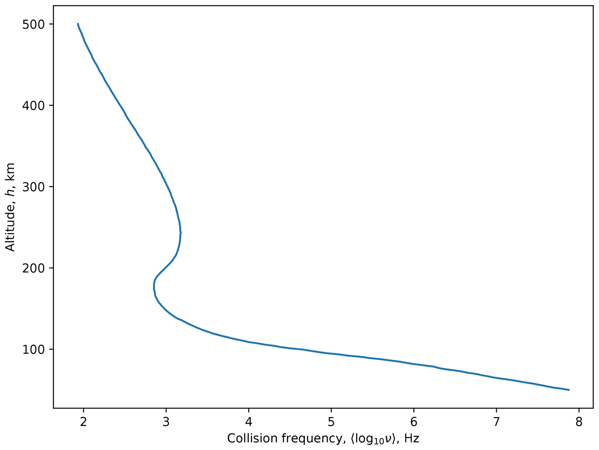
This equation is widely used when modelling CNA (Hargreaves, 1969; Hunsucker and Hargreaves, 2002). The electron collision frequency is ultimately a function of neutral density and electron temperature. However, at any given altitude, the electron temperature typically changes very little, and variations in absorption are attributed to variations in electron density. A measure of the electron collision frequency, ν, is required. For this the results collated by Aggarwal et al. (1979, Fig. 7) were used, a look-up table was generated and a linear interpolation was used for determining intermediate values. This gives a realistic electron collision frequency for any given height in the approximate range of 50–500 km and is shown in Fig. 1.

Figure 1 The model of electron collision frequency $\mathit{\nu }={\mathit{\nu }}_{\mathrm{en}}+{\mathit{\nu }}_{\mathrm{ei}}$ from Aggarwal et al. (1979).

2.1 Specification of the forward model

The forward problem is defined as follows:

$$\begin{array}{}\text{(4)}& \mathbf{d}=\mathbf{Gm}+\mathit{\eta },\end{array}$$

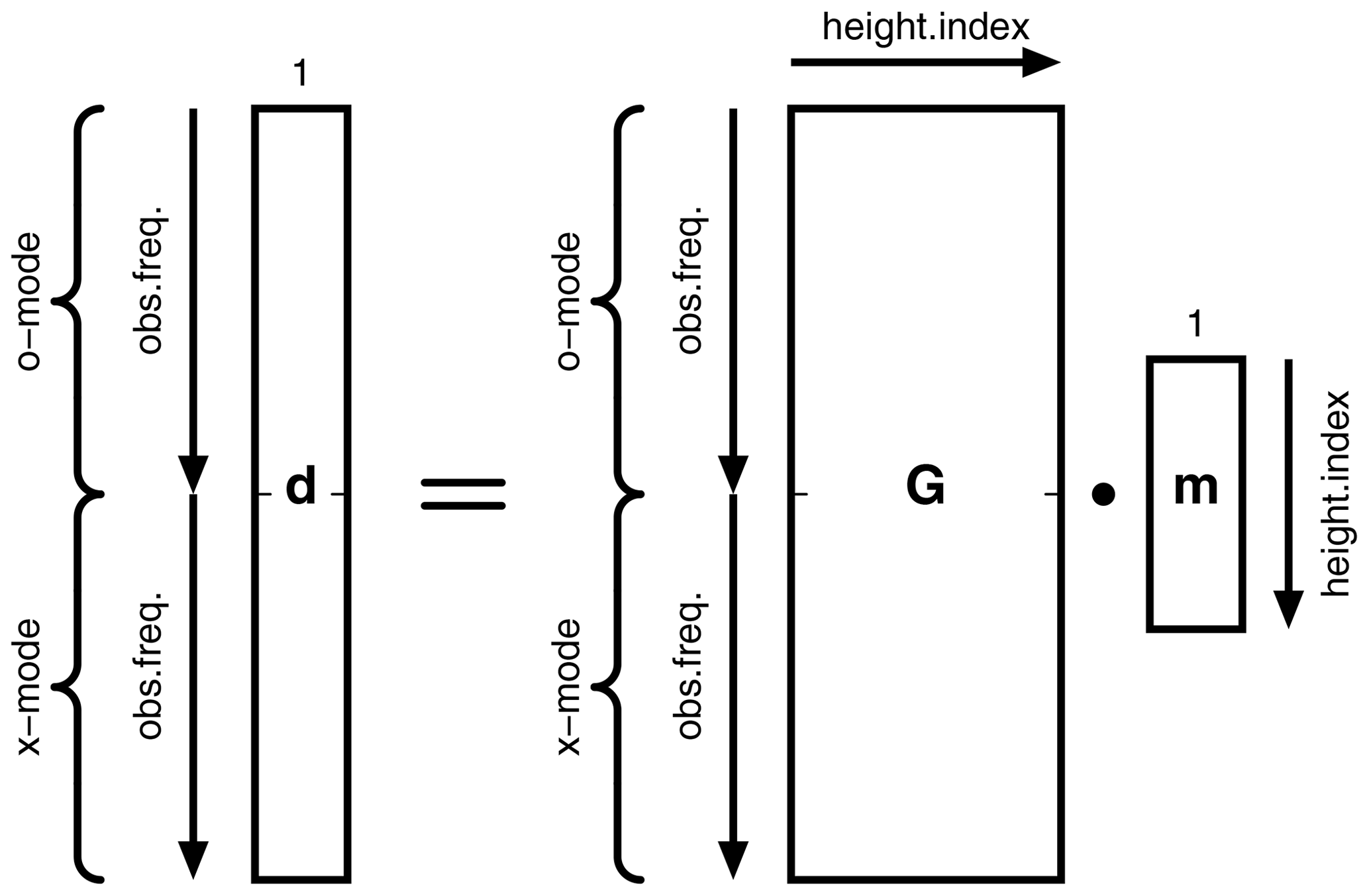
where d is the data, G is the forward model and m is the model. For generating sample data, an error term, η, is used, which follows a normal distribution. In this study, the data, d, is the absorption measured at a given frequency and polarisation mode. The model, m, is the electron density, N_e(h), for a given height, h. The range of heights used can be varied, but for this initial test a range of 65–110 km was selected, which spans the D region and includes lower altitudes down to 50 km (which would be subject to electron density enhancements in the event of hard precipitation).

The forward model, G, is a linear algebraic representation of the riometry equation (Eq. 3). The riometry equation is continuous, so it is discretised as follows:

$$\begin{array}{}\text{(5)}& A=\mathrm{4.611}\times {\mathrm{10}}^{-\mathrm{5}}\sum _{h=h_{\min }}^{h_{\max }}{\displaystyle \frac{N_{\mathrm{e}}\mathit{\nu }}{{\mathit{\nu }}^{\mathrm{2}}+(\mathit{\omega }\pm {\mathit{\omega }}_L{)}^{\mathrm{2}}}}\mathrm{\Delta }h\left(\mathrm{dB}\right).\end{array}$$

This can be expressed in matrix form as follows.

$$\begin{array}{ll}\text{(6)}& {\displaystyle }& {\displaystyle }\left[\begin{array}{c}{A}_{o_{\mathrm{1}}}\\ A_{o_{\mathrm{2}}}\\ \mathrm{⋮}\\ A_{o_N}\\ \\ A_{x_{\mathrm{1}}}\\ A_{x_{\mathrm{2}}}\\ \mathrm{⋮}\\ A_{x_N}\end{array}\right]={\displaystyle }& {\displaystyle }\left[\begin{array}{cccc}\frac{k{\mathit{\nu }}_{{}_{\mathrm{1}}}\mathrm{\Delta }h}{{\mathit{\nu }}_{\mathrm{1}}^{\mathrm{2}}+({\mathit{\omega }}_{\mathrm{1}}+{\mathit{\omega }}_L{)}^{\mathrm{2}}}& \frac{k{\mathit{\nu }}_{{}_{\mathrm{2}}}\mathrm{\Delta }h}{{\mathit{\nu }}_{\mathrm{2}}^{\mathrm{2}}+({\mathit{\omega }}_{\mathrm{1}}+{\mathit{\omega }}_L{)}^{\mathrm{2}}}& \mathrm{\dots }& \frac{k{\mathit{\nu }}_{{}_M}\mathrm{\Delta }h}{{\mathit{\nu }}_M^{\mathrm{2}}+({\mathit{\omega }}_{\mathrm{1}}+{\mathit{\omega }}_L{)}^{\mathrm{2}}}\\ \frac{k{\mathit{\nu }}_{{}_{\mathrm{1}}}\mathrm{\Delta }h}{{\mathit{\nu }}_{\mathrm{1}}^{\mathrm{2}}+({\mathit{\omega }}_{\mathrm{2}}+{\mathit{\omega }}_L{)}^{\mathrm{2}}}& \frac{k{\mathit{\nu }}_{{}_{\mathrm{2}}}\mathrm{\Delta }h}{{\mathit{\nu }}_{\mathrm{2}}^{\mathrm{2}}+({\mathit{\omega }}_{\mathrm{2}}+{\mathit{\omega }}_L{)}^{\mathrm{2}}}& \mathrm{\dots }& \frac{k{\mathit{\nu }}_{{}_M}\mathrm{\Delta }h}{{\mathit{\nu }}_M^{\mathrm{2}}+({\mathit{\omega }}_{\mathrm{2}}+{\mathit{\omega }}_L{)}^{\mathrm{2}}}\\ \mathrm{⋮}& \mathrm{⋮}& \mathrm{\ddots }& \mathrm{⋮}\\ \frac{k{\mathit{\nu }}_{{}_{\mathrm{1}}}\mathrm{\Delta }h}{{\mathit{\nu }}_{\mathrm{1}}^{\mathrm{2}}+({\mathit{\omega }}_N+{\mathit{\omega }}_L{)}^{\mathrm{2}}}& \frac{k{\mathit{\nu }}_{{}_{\mathrm{2}}}\mathrm{\Delta }h}{{\mathit{\nu }}_{\mathrm{2}}^{\mathrm{2}}+({\mathit{\omega }}_N+{\mathit{\omega }}_L{)}^{\mathrm{2}}}& \mathrm{\dots }& \frac{k{\mathit{\nu }}_{{}_M}\mathrm{\Delta }h}{{\mathit{\nu }}_M^{\mathrm{2}}+({\mathit{\omega }}_N+{\mathit{\omega }}_L{)}^{\mathrm{2}}}\\ \\ \frac{k{\mathit{\nu }}_{{}_{\mathrm{1}}}\mathrm{\Delta }h}{{\mathit{\nu }}_{\mathrm{1}}^{\mathrm{2}}+({\mathit{\omega }}_{\mathrm{1}}-{\mathit{\omega }}_L{)}^{\mathrm{2}}}& \frac{k{\mathit{\nu }}_{{}_{\mathrm{2}}}\mathrm{\Delta }h}{{\mathit{\nu }}_{\mathrm{2}}^{\mathrm{2}}+({\mathit{\omega }}_{\mathrm{1}}-{\mathit{\omega }}_L{)}^{\mathrm{2}}}& \mathrm{\dots }& \frac{k{\mathit{\nu }}_{{}_M}\mathrm{\Delta }h}{{\mathit{\nu }}_M^{\mathrm{2}}+({\mathit{\omega }}_{\mathrm{1}}-{\mathit{\omega }}_L{)}^{\mathrm{2}}}\\ \frac{k{\mathit{\nu }}_{{}_{\mathrm{1}}}\mathrm{\Delta }h}{{\mathit{\nu }}_{\mathrm{1}}^{\mathrm{2}}+({\mathit{\omega }}_{\mathrm{2}}-{\mathit{\omega }}_L{)}^{\mathrm{2}}}& \frac{k{\mathit{\nu }}_{{}_{\mathrm{2}}}\mathrm{\Delta }h}{{\mathit{\nu }}_{\mathrm{2}}^{\mathrm{2}}+({\mathit{\omega }}_{\mathrm{2}}-{\mathit{\omega }}_L{)}^{\mathrm{2}}}& \mathrm{\dots }& \frac{k{\mathit{\nu }}_{{}_M}\mathrm{\Delta }h}{{\mathit{\nu }}_M^{\mathrm{2}}+({\mathit{\omega }}_{\mathrm{2}}-{\mathit{\omega }}_L{)}^{\mathrm{2}}}\\ \mathrm{⋮}& \mathrm{⋮}& \mathrm{\ddots }& \mathrm{⋮}\\ \frac{k{\mathit{\nu }}_{{}_{\mathrm{1}}}\mathrm{\Delta }h}{{\mathit{\nu }}_{\mathrm{1}}^{\mathrm{2}}+({\mathit{\omega }}_N-{\mathit{\omega }}_L{)}^{\mathrm{2}}}& \frac{k{\mathit{\nu }}_{{}_{\mathrm{2}}}\mathrm{\Delta }h}{{\mathit{\nu }}_{\mathrm{2}}^{\mathrm{2}}+({\mathit{\omega }}_N-{\mathit{\omega }}_L{)}^{\mathrm{2}}}& \mathrm{\dots }& \frac{k{\mathit{\nu }}_{{}_M}\mathrm{\Delta }h}{{\mathit{\nu }}_M^{\mathrm{2}}+({\mathit{\omega }}_N-{\mathit{\omega }}_L{)}^{\mathrm{2}}}\end{array}\right]\\ {\displaystyle }& {\displaystyle }\cdot \left[\begin{array}{c}{m}_{\mathrm{1}}\\ m_{\mathrm{2}}\\ \mathrm{⋮}\\ m_M\end{array}\right]\end{array}$$

In Eq. (6), $m_{\mathrm{1}},m_{\mathrm{2}},\mathrm{\dots }{m}_M$ are the model parameters, i.e. the electron density m_i=N_e(h), where i is the height array index for a given height, h. The size of a height increment, Δh, is the distance between heights h_i and h_i+1. The data are the measured absorptions in decibels for the _o- and _x-mode polarisations, $A_{{\mathrm{o}}_j}$ and $A_{{\mathrm{x}}_j}$, respectively, where j is the frequency channel array index. The series ${\mathit{\nu }}_{\mathrm{1}},{\mathit{\nu }}_{\mathrm{2}},\mathrm{\dots }{\mathit{\nu }}_{{}_M}$ is the electron collision frequency profile, ν_i=ν(h), where i is the height array index for a given height, h. A look-up table is used for the collision frequencies (Fig. 1). In order to declutter the representation, the symbol k is used for the riometry constant from Eq. (3), with $k=\mathrm{4.611}\times {\mathrm{10}}^{-\mathrm{5}}$. A diagrammatic representation of the matrices and their dimensions is shown in Fig. 2.

Figure 2 Illustration of the matrix dimensions of the model (see Eq. 6).

The angular gyrofrequency is a function of the magnetic field, which is effectively constant over the range of heights being studied. The magnetic field expected in the sub-polar regions of the Earth is typically 50 µT, giving an electron gyro frequency of ${\mathit{\omega }}_H=\mathrm{2}\mathit{\pi }\times \mathrm{1.4}\times {\mathrm{10}}^{\mathrm{6}}$ Hz. Ions and other larger species have much higher masses, resulting in gyro frequencies that can be neglected (McKay, 2018). Field-aligned observations are assumed (where ω_L=ω_H), as this is the best-case scenario.

2.2 Example electron density profiles

To test the model and the ability to solve it, synthetic data are generated for the altitude ranges that could be expected in a physical situation. The frequency range chosen, 15–78 MHz, extends from the penetration cut-off frequency to just below the FM radio band (a practical limit for riometers due to interference).

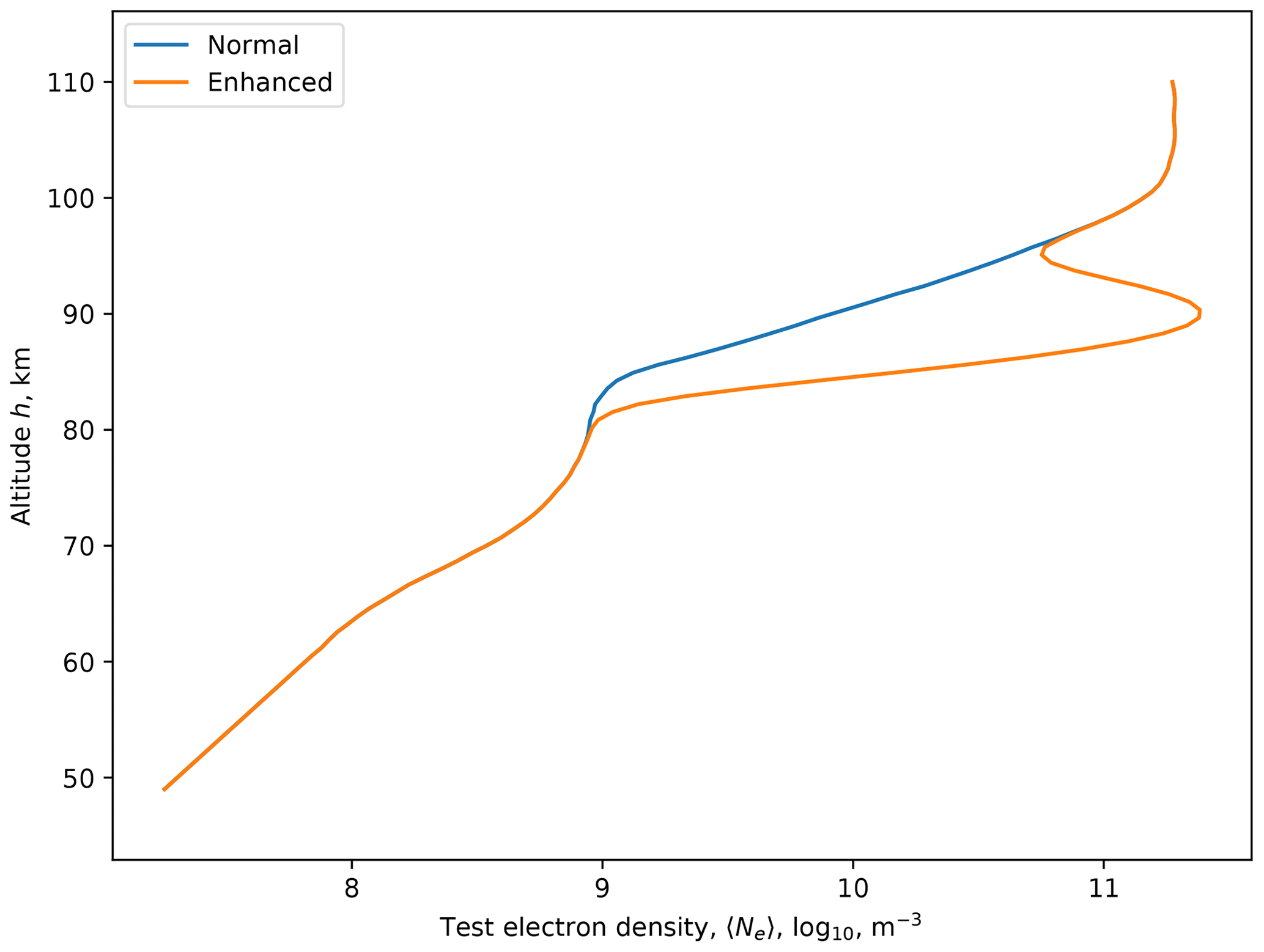
An electron density profile from Gnanalingam and Kane (1975) was used as a basis (the “normal” profile shown in Fig. 3). In order to simulate lower altitudes, a simple interpolation between the lowest value from Gnanalingam and Kane (1975) and that of Jespersen et al. (1964) was made. This is a safe assumption, as the electron densities at these altitudes are several orders of magnitude lower than those found in the D and E regions.

Although there is always some level of absorption imposed by the atmosphere on incoming radio waves, it is the enhanced absorption that is of particular interest and is also the target measurement for riometers. The electron density enhancements in the ionosphere are often the result of substorms (Hunsucker and Hargreaves, 2002). Earlier studies (e.g. Jussila et al., 2004) have determined that neither plasma instabilities nor enhanced electron temperatures in the E region play a significant role in causing the CNA and concluded that CNA is caused by energetic electron precipitation reaching down into the D region, with a maximum between 80 and 90 km.

An enhancement of approximately 1 order of magnitude is made at an altitude of 90 km, with a full width at half maximum of 10 km. This is applied to the “normal profile” based on Gnanalingam and Kane (1975) to simulate the “enhanced profile”. These normal and enhanced profiles are shown in Fig. 3.

Figure 3 Electron density profiles for normal and enhanced conditions.

2.3 Application of the forward model

With a model electron density profile it is now possible to apply the forward model, G, to it to generate the sample data. This has been done for both the normal and enhanced profiles, and the results are shown in Fig. 4.

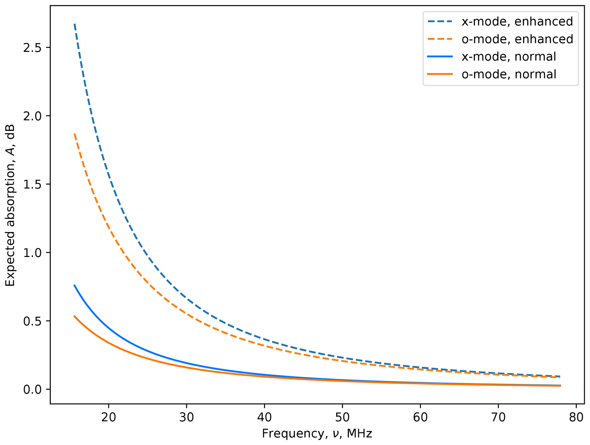
Figure 4 Expected CNA from normal and enhanced conditions for both _x-mode and _o-mode radio waves. The horizontal axis shows the observing radio frequency, $\mathit{\nu }=\mathit{\omega }/\mathrm{2}\mathit{\pi }$, in megahertz.

The first thing to note from these data is that there is already a background amount of absorption between the normal and enhanced electron density profiles. A riometric measurement, on the grounds that it uses a quiet-day subtraction technique, is measuring the difference in absorption between the normal and enhanced conditions.

The effect of absorption decreases with radio frequency, which is the reason why many riometers operate in the 30–40 MHz range. Above this, absorption is comparable to noise levels (±0.1 dB) from typical instruments.

The strongest absorption effects are at the lower frequencies, but when cross-referencing against the radio frequency environment of suitable instruments (e.g. McKay-Bukowski et al., 2015, Fig. 7), frequencies below 25 MHz are fraught with short-wave radio interference, making their use impractical.

3 Inverse analysis

The method used to solve this inverse problem is singular value decomposition (SVD). Equation (4) is refactored as follows:

$$\begin{array}{}\text{(7)}& \mathbf{G}={\mathbf{USV}}^T,\end{array}$$

where U is an N-by-N orthogonal matrix with columns that are unit basis vectors in the data space, V is an M-by-M orthogonal matrix with columns that are basis vectors in the model space and S is an N-by-M diagonal matrix; the diagonal elements are the singular values. The SVD is used to compute the Moore–Penrose pseudo-inverse, such that

$$\begin{array}{}\text{(8)}& {\mathbf{G}}^{\mathit{†}}={\mathbf{V}}_p{\mathbf{S}}_p^{-\mathrm{1}}{\mathbf{U}}_p^T,\end{array}$$

where V_p represents the first p columns of V (and similarly for the other matrices). This is a valid simplification, as the singular values of S are typically arranged in decreasing magnitude along the diagonal by assuming that S:

$$\begin{array}{}\text{(9)}& \mathbf{S}=\left[\begin{array}{cc}{\mathbf{S}}_p& \mathrm{0}\\ \mathrm{0}& \mathrm{0}\end{array}\right]\end{array}$$

As columns ≥p in U and V are multiplied by zeros in the S matrix, the matrices can be treated as orthonormal, with the simplifications that can be applied to orthonormal matrices. Thus the generalised form becomes

$$\begin{array}{}\text{(10)}& {\mathbf{G}}^{\mathit{†}}={\mathbf{V}}_p{\mathbf{S}}_p^{-\mathrm{1}}{\mathbf{U}}_p^T.\end{array}$$

The proof for which is given in Aster et al. (2011, chap. 3).

3.1 Interpretation of the SVD products

Following the singular value decomposition, the V matrix can be represented as an image to gain an understanding of the determinism of the solution. This is shown in Fig. 5. There is a large noise component throughout most of the solution, with only the first few columns showing non-noise structure.

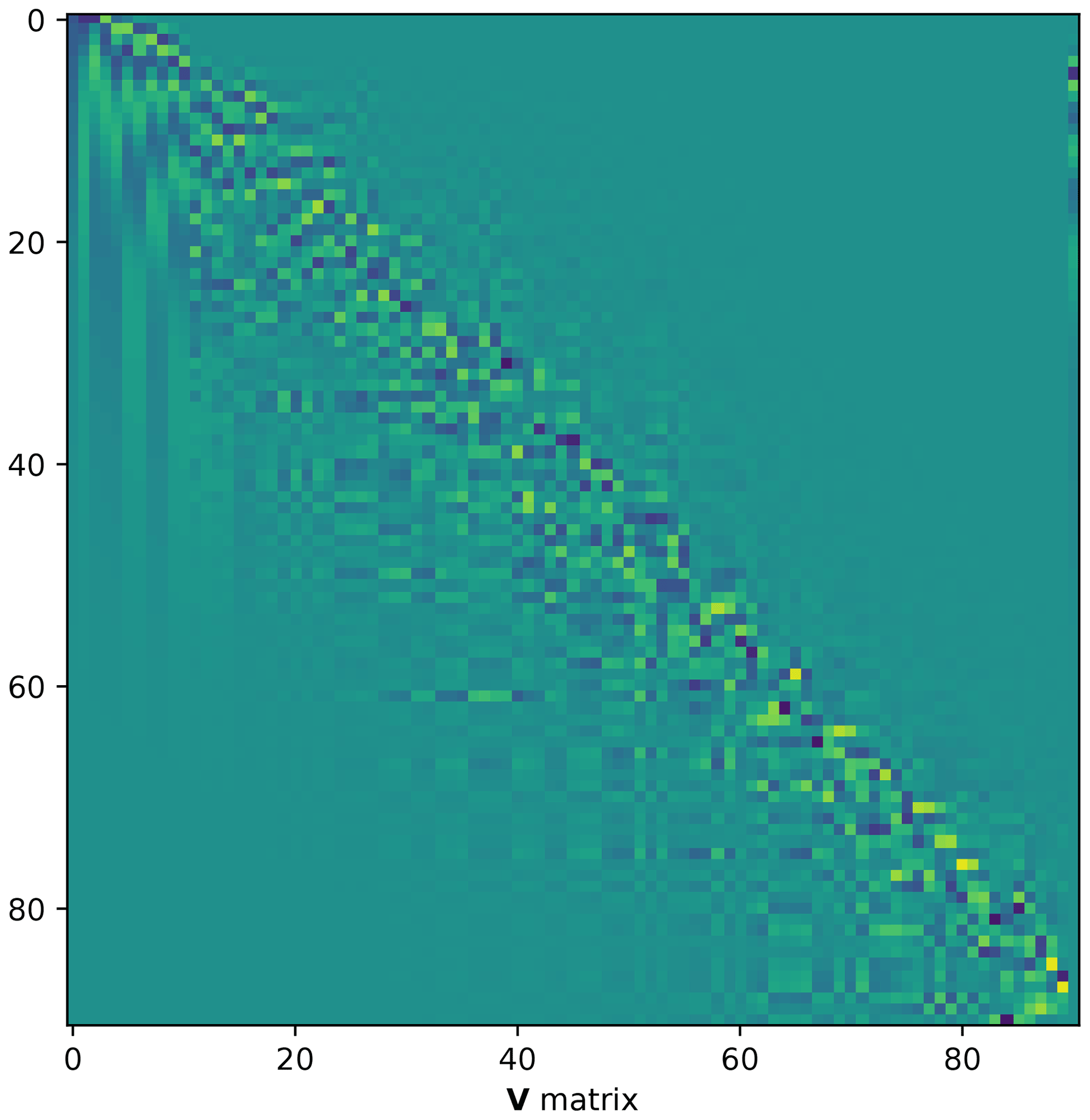
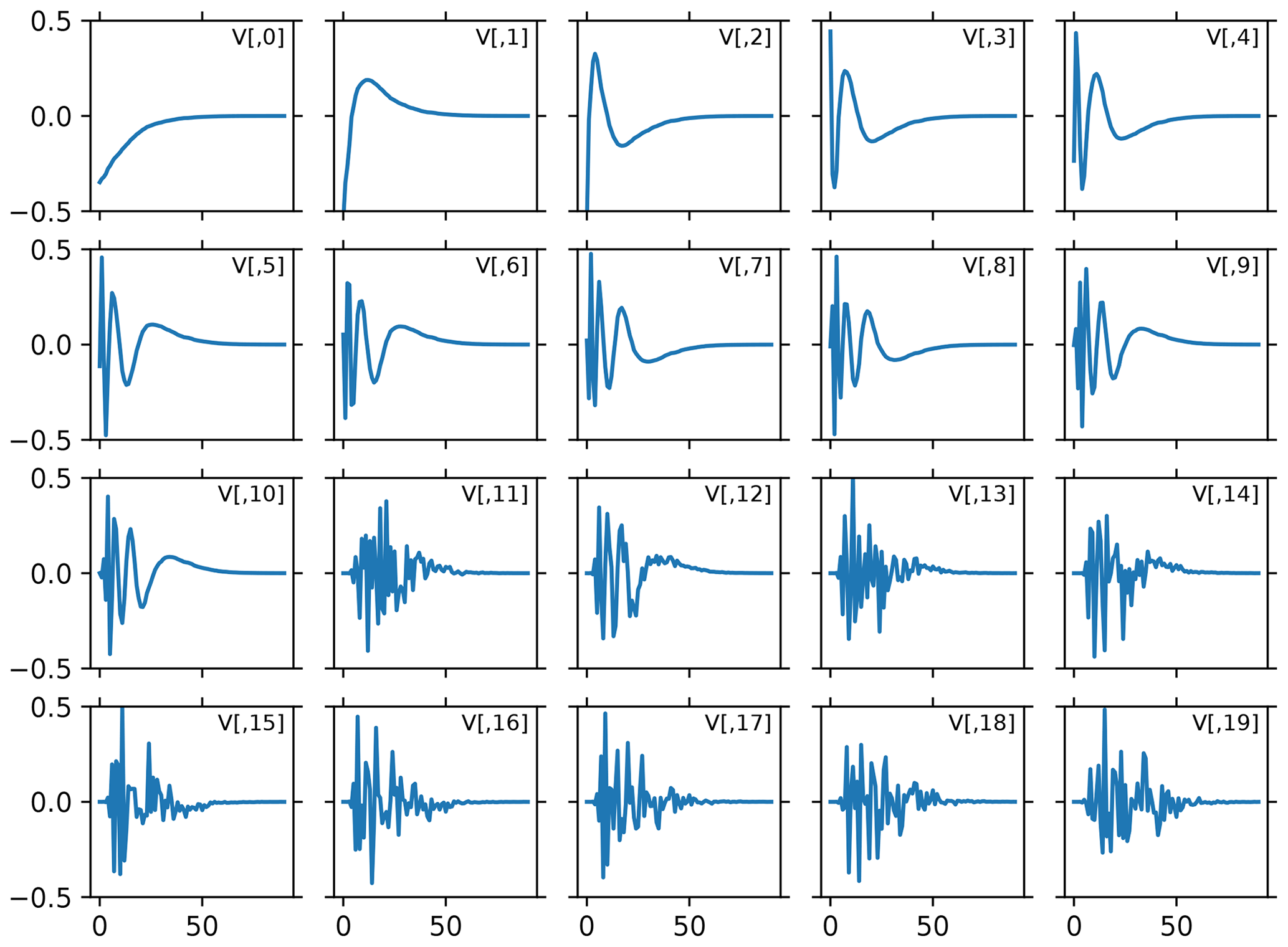
Figure 5 Image representation of the V matrix. The first 11 columns show non-noise structures. These are shown in Fig. 6 with scale information .

The columns are the basis functions, with the first 20 of these being shown with scale information in Fig. 6. As can be seen, the first few basis functions have structure, but thereafter the noise becomes increasingly dominant.

Figure 6 The first 20 basis functions from the V matrix.

As Eq. (5) and thus the forward matrix system represented by Eq. (6) are linear systems, it is possible to assess them for rank deficiency – namely, insufficient information to extract the parameters of the desired model. Although higher-order terms have non-zero values, these are extremely small and represent round-off errors and floating-point number quantisation errors.

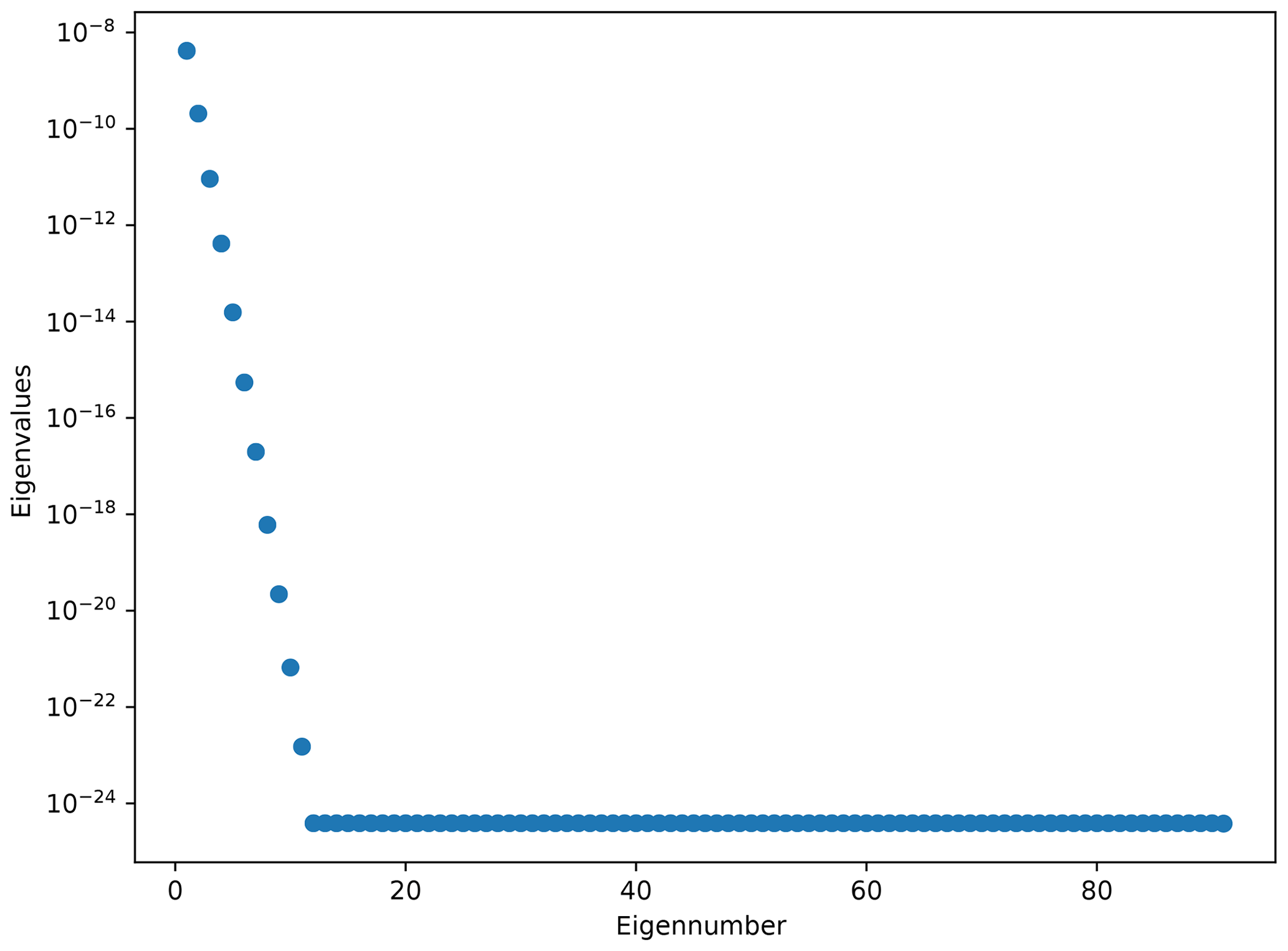
In Fig. 7, the eigenvalues of the S matrix are plotted as a function of the eigennumber to create a so-called “L-curve”. As the values are so tiny and cover a large dynamic range, a log-linear plot is used to highlight the salient features and as a result distort the original L form.

Figure 7 Eigenvalue of the S matrix plotted as function of the eigennumber.

Typically, the technique is to truncate the effectively zero singular values. This produces a least-squares solution of limited resolution. Although rank-deficient problems can be solved by applying a generalised inverse solution, there is insufficient information to recover the complexity of the model – in this application case this is the electron density profile.

Examination of Fig. 7 shows that there are approximately 2 orders of magnitude difference between the first and second term. Even if there was information contained within those terms (and the basis functions suggest there might be to the fifth term), the effect that this has on the model determination is negligible.

Terms after the 11th term are below 10⁻²⁴. Compared to the first term (just below 10⁻⁸), this represents a 10¹⁶ dynamic-range shift. This is equivalent to the numerical dynamic range of the double-precision floating-point number representation (bits $\mathrm{2}-\mathrm{53}\approx \mathrm{1.11}\times {\mathrm{10}}^{-\mathrm{16}}$). Thus, these higher terms are equivalent to the least significant bit of the floating-point representation and thus can be considered to be numerically zero.

As a result, it can be hypothesised that any number of model solutions could be formulated that would result in a superficial fit of the data. If this hypothesis holds, then it demonstrates the non-uniqueness of the solution, and thus it will verify that the original inverse problem is ill posed. Reducing the number of terms used still does not constrain the model, and reduction to the lowest term is equivalent to a single-frequency riometer providing a single absorption measurement.

3.2 Inversion

To test the hypothesis, two test model data sets are formulated using literature-sourced data (Sect. 2.2) and a data set that can be derived by applying the forward model to those data (Sect. 2.3). These data sets include one for normal quiet ionospheric conditions, d_nor, and one for enhanced conditions, d_enh. The forward matrix, G, was applied and a normally distributed noise term, η, added.

$$\begin{array}{}\text{(11)}& {\displaystyle }\mathit{\eta }=\mathcal{N}(\mathrm{0},{\mathit{\sigma }}^{\mathrm{2}});\mathrm{where}\mathit{\sigma }=\mathrm{0.1}\text{(12)}& {\displaystyle }{\mathbf{d}}_{\mathrm{nor}}={\mathbf{Gm}}_{\mathrm{nor}}+\mathit{\eta }\text{(13)}& {\displaystyle }{\mathbf{d}}_{\mathrm{enh}}={\mathbf{Gm}}_{\mathrm{enh}}+\mathit{\eta }\end{array}$$

Recovery of the original model was then attempted using several different techniques. These used standard library functions provided by the Python numpy (Eq. 14) and scipy (Eq. 15) packages (Harris et al., 2020), as well as a direct maximum a posteriori estimate (Eq. 16) and Tikhonov regularised solution (Eq. 17). For the normal ionosphere case, these are

$$\begin{array}{}\text{(14)}& {\displaystyle }{\mathbf{m}}_{{}_{\mathrm{LS}}}=\mathtt{linalg}.\mathtt{lstsq}(\mathtt{G},\mathtt{d}),\text{(15)}& {\displaystyle }{\mathbf{m}}_{{}_{\mathrm{NNLS}}}=\mathtt{scipy}.\mathtt{optimise}.\mathtt{nnls}(\mathtt{G},\mathtt{d}),\text{(16)}& {\displaystyle }{\mathbf{m}}_{\mathrm{est}}=({\mathbf{G}}^T{\mathbf{\Sigma }}^{-\mathrm{1}}\mathbf{G}{)}^{-\mathrm{1}}{\mathbf{G}}^T{\mathbf{\Sigma }}^{-\mathrm{1}}\mathbf{d},\text{(17)}& {\displaystyle }{\mathbf{m}}_{\mathrm{tik}}={\mathbf{VS}}^{\mathit{†}}{\mathbf{U}}^T\mathbf{d}.\end{array}$$

Figure 8 shows the comparison of the original model and the data generated from the inverse solutions.

Figure 8 Application of the forward models to different solutions. The black “nominal” line does not readily appear as the “estimate” is collinear with it. The horizontal axis is the observing radio frequency, $\mathit{\nu }=\mathit{\omega }/\mathrm{2}\mathit{\pi }$.

In Fig. 8, the “nominal” data are shown with a solid black line. This is the original electron density profile during normal ionospheric conditions when applying the forward model without noise (Sect. 2.2). The noisy blue data are the same but with the noise term, η, applied (Eq. 12). The dashed traces are for the maximum a posteriori estimate and Tikhonov-regularised solutions, when transformed with the forward matrix:

$$\begin{array}{}\text{(18)}& {\displaystyle }{\mathbf{d}}_{\mathrm{est}}={\mathbf{Gm}}_{\mathrm{est}},\text{(19)}& {\displaystyle }{\mathbf{d}}_{\mathrm{tik}}={\mathbf{Gm}}_{\mathrm{tik}}.\end{array}$$

Residuals can be calculated by subtracting the original noiseless data from these inverse problem solutions, for example:

$$\begin{array}{}\text{(20)}& {\mathbf{r}}_{\mathrm{est}}={\mathbf{d}}_{\mathrm{est}}-\mathbf{d}.\end{array}$$

These are plotted for the two propagation modes (_o mode and _x mode) for different solution forms (Eqs. 14–17), as shown in Fig. 9. The fact that the residuals are all effectively the same indicates that all methods are recovering the same solution and that the algorithms are mathematically equivalent.

Figure 9 Residuals between data from original and determined models. The solid line corresponds to the _o mode, and the dashed line is for the _x mode. All four methods give the same result for the given mode. The lines are superimposed, which is why only one colour seemingly appears, even though all methods are being plotted, as per the legend.

Note also that the residual values are small, <0.1 dB, which is considered the noise limit of current instrumentation. The residuals are larger at lower frequencies, which is a result of the increased relative importance of the noise with respect to the signal.

Figure 10 shows the maximum a posteriori data together with the original “true” data.

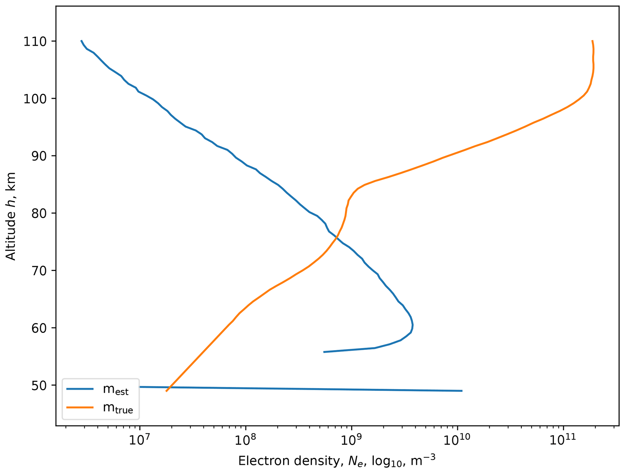
Figure 10 Fit of an electron density profile (SVD method). The discontinuity corresponds to the minimum altitude of the input collision frequency profile.

The two profiles bear no resemblance. However, the m_est does match the same general shape of the collision frequency profile. What is happening is that the collision frequency is a dominant input form, and the solution naturally aligns itself to it. In considering the different methods for solving the inverse problem, all of them give stable, repeatable results based on the input data. The variation between individual solution methods is close to the floating-point quantisation noise. However, even though it satisfies the stability criteria for a well-posed problem, the mathematical examination still implies that it is possible to formulate non-unique solutions.

If the model solution matches the same form as the collision frequency profile (which is an input function), it should in principle be possible to fit any input function to measured absorption.

3.3 Inversion of arbitrary functions

To demonstrate the ill-posed nature of the inverse problem, a series of arbitrary functions was fitted to simulated electron density profiles. In this case,

$$\begin{array}{}\text{(21)}& \mathbf{d}={\mathbf{G}}_{\mathrm{s}}\mathbf{m},\end{array}$$

where d is the simulated data and G_s is the forward matrix for a specific shape function, S(h). Because the shape function has an altitude profile (e.g. a Gaussian can be specified to have a peak at a pre-determined altitude), then the only free parameter is the scaling of the function. Thus, S is effectively a scalar.

The data, d, are a function of frequency and polarisation mode, but the forward model collapses to a single line as follows.

$$\begin{array}{}\text{(22)}& {\mathbf{G}}_{\mathrm{s}}=\left[\begin{array}{c}\frac{k{\mathit{\nu }}_{{}_{\mathrm{1}}}s\left(h_{\mathrm{1}}\right)\mathrm{\Delta }h}{{\mathit{\nu }}_{\mathrm{1}}^{\mathrm{2}}+({\mathit{\omega }}_{\mathrm{1}}+{\mathit{\omega }}_L{)}^{\mathrm{2}}}+\mathrm{\cdots }+\frac{k{\mathit{\nu }}_{{}_{\mathrm{1}}}s\left(h_H\right)\mathrm{\Delta }h}{{\mathit{\nu }}_{\mathrm{1}}^{\mathrm{2}}+({\mathit{\omega }}_{\mathrm{1}}+{\mathit{\omega }}_L{)}^{\mathrm{2}}}\\ +\frac{k{\mathit{\nu }}_{{}_{\mathrm{1}}}s\left(h_{\mathrm{1}}\right)\mathrm{\Delta }h}{{\mathit{\nu }}_{\mathrm{1}}^{\mathrm{2}}+({\mathit{\omega }}_{\mathrm{1}}-{\mathit{\omega }}_L{)}^{\mathrm{2}}}+\mathrm{\cdots }+\frac{k{\mathit{\nu }}_{{}_{\mathrm{1}}}s\left(h_H\right)\mathrm{\Delta }h}{{\mathit{\nu }}_{\mathrm{1}}^{\mathrm{2}}+({\mathit{\omega }}_{\mathrm{1}}-{\mathit{\omega }}_L{)}^{\mathrm{2}}}\end{array}\right]\end{array}$$

Here, s(h) is the value of the shape function (where the parameter is the altitude height, h). The other terms are as per Eq. (6).

As an example of how these operate in practice, two Gaussian functions were chosen. The Gaussian width parameter in both cases was σ=5, and the peak height was set to μ=70 and μ=100 km for the low and high cases, respectively. Absorption profiles were created using the physical models indicated in the previous section. Thus, a quasi-real atmospheric profile for both normal and enhanced ionospheric conditions could be created. For both cases, the arbitrary shape functions were fitted, which are shown, together with the results, in Figs. 11 and 12 for the low and high Gaussian profiles, respectively. With the fitted result, there are also the residuals for the normal and enhanced ionospheric conditions. The residuals have been plotted with the same vertical scaling to allow easy comparison. The range of these scales was set to ±0.1 dB, corresponding to the approximate riometry noise that could be anticipated from real experimental data (e.g. McKay et al., 2015).

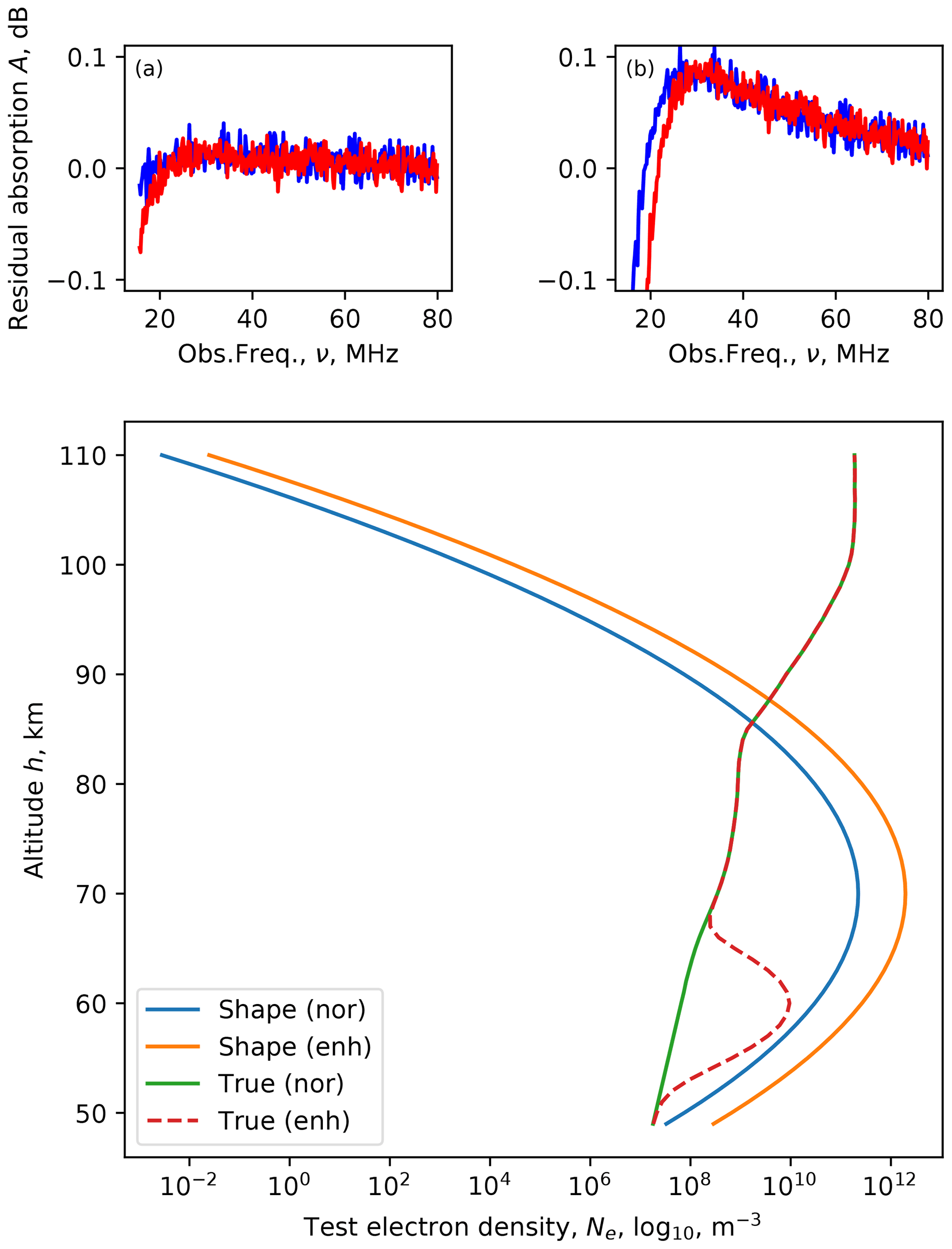
Figure 11 Fitting a 70 km peak Gaussian electron density profile to simulated normal (nor) and enhanced (enh) ionospheric profile data. The residuals are shown in the two top panels as a function of the observing frequency: (a) normal and (b) enhanced, with the _o mode shown in blue and the _x mode in red.

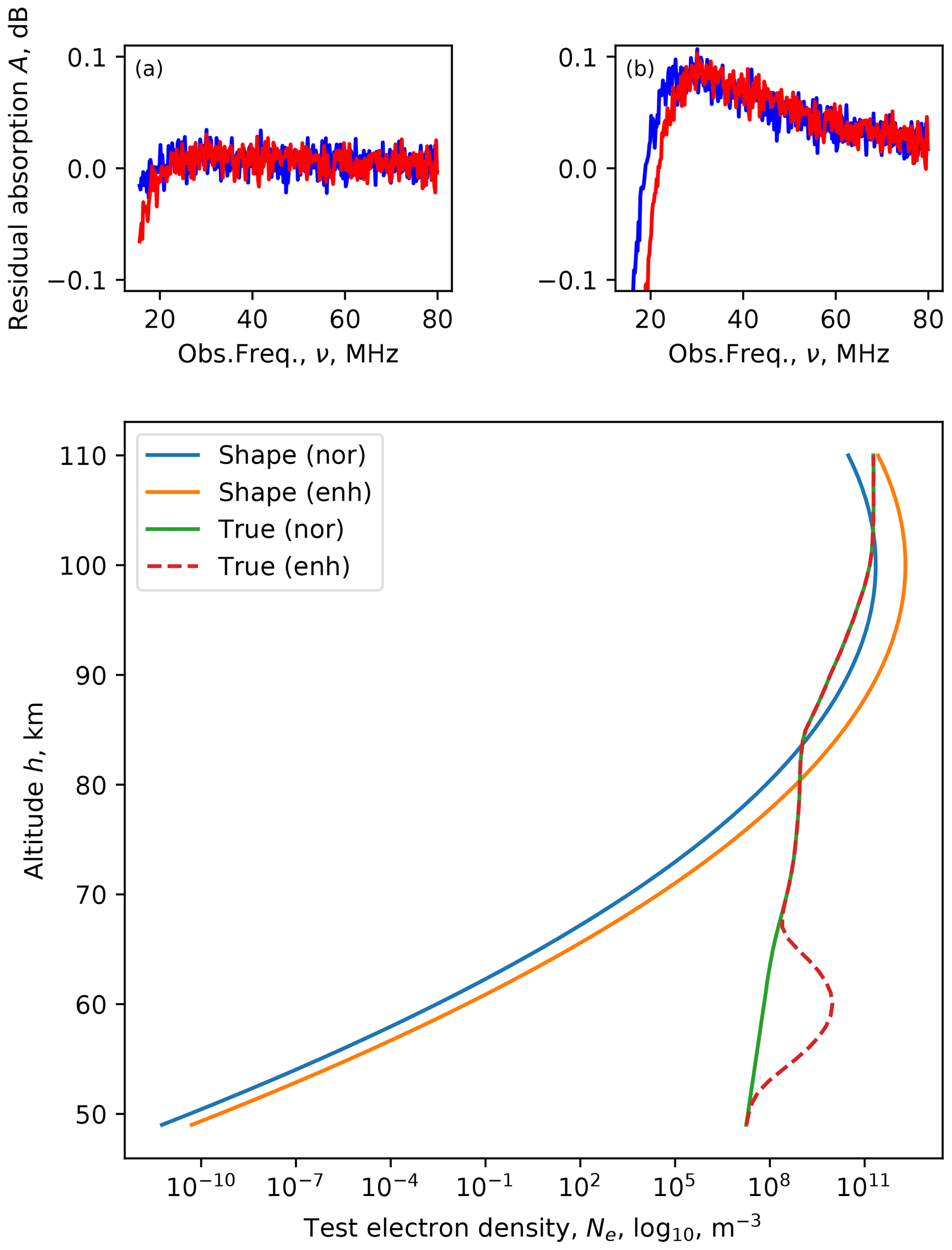
Figure 12 Fitting a 100 km peak Gaussian electron density profile to simulated normal and enhanced ionospheric profile data. The residuals are shown in the two top panels as a function of the observing frequency: (a) normal and (b) enhanced, with the _o mode shown in blue and the _x mode in red.

In both the low- and high-Gaussian cases the residuals were below the expected noise limit of the riometer. Additionally, there was no significant difference between the two. The implication of this is that the inverse method is incapable of determining the altitude of a Gaussian profile.

Additional testing showed that similar results could be found with other forms (delta functions, gradients, constant offsets, etc.). In all cases, there is insufficient information to be able to say anything meaningful about the height distribution of the electron density profile, given the observed absorption over the 18–80 MHz range for _o- and _x-mode propagation.

3.4 Remarks

The original work done on the inversion problem was by Parthasarathy et al. (1963). In that work, three parameters were fitted. Since then, various authors have attempted linear least-squares fitting to determine the maximum likelihood polynomial coefficients (e.g. Belikovich et al., 1964). However, as has been shown, even in the best-case field-aligned propagation scenario, there is insufficient information to discern a single parameter (Gaussian height) fit from the data. The implication is that this line of research has been mathematically demonstrated to be unattainable. Nevertheless, there are still other advantages of multi-frequency riometry measurements. Firstly, it permits more independent measurements of power for the same antenna.

Multi-frequency riometry also validates the idea that detected absorption is the result of electron content in the ionosphere. This is because any absorption from the atmosphere will be a function of frequency (ω), approximating $A\left(\mathit{\omega }\right)=A_{\mathrm{0}}/{\mathit{\omega }}^{\mathrm{2}}$. This makes the instrument robust against natural and artificial forms of radio interference. In the case of natural interference, these may be useful scientific measurements in their own right, such as observation of strong solar radio emissions or Jovian decametric emissions.

Accurate electron density profile measurements therefore require a strong additional a priori assumption of the electron density profile, for example a parameterised model for the ionisation source or supplementary measurements such as those from an incoherent scatter radar. The results of this study indicate that the shape of the absorption spectrum does not provide any distinguishable information on the electron density height profile from typical substorm electron precipitation. However, exceptional cases may still exist where a remarkable part of the ionisation reaches down to below 50 km altitude. From the known ionisation sources, at least the major solar proton events can ionise the atmosphere down to stratospheric altitudes and hence be expected to potentially change the spectral shape (Verronen, 2006). It is also worth mentioning that if trying to distinguish this effect (or any other anomalous ionisation in the deep D-region) from the absorption spectrum, one needs to consider the signal-to-noise ratio (SNR) of the instrument carefully. Although the SNR issue is not the primary focus of this paper, it is important to mention because (1) a finite SNR always reduces the absorption detected (the lower the SNR, the lower the absorption measured), (2) the amount of this reduction depends on the magnitude of the absorption itself (the higher the real absorption, the more SNR reduces the detection) and (3) the SNR is frequency dependent for any real spectral riometer instrument. Hence, without taking the SNR into account, the spectral shape apparently always changes when the absorption changes, regardless of the ionisation altitude.

4 Conclusions

This study has considered the determination of atmospheric electron density using multi-frequency, multi-polarisation, cosmic noise absorption data (the spectral riometry technique). It has examined the solutions that can be obtained (using both real and modelled data) and has considered whether the problem is “well posed”.

The determination of electron density profiles, primarily in the D and E region of the ionosphere, can be attempted using an inverse problem technique and radio absorption data. The absorption is measured over the 15–78 MHz range, which is the practical range that can be achieved with existing instrumentation.

A forward model was developed based on the riometry equation. Using a singular-value decomposition, the electron density profile was solved. However, the profile followed the collision frequency parameter, indicating that it was not well determined and was thus strongly influenced by other solutions. The assessment of the eigenvalues indicated that there are only a few significant basis functions, and thus no real information could be recovered.

This was further tested by finding maximum-likelihood estimates for arbitrary profile functions. The residuals were of similar form and were contained within the noise range that could be expected from typical riometry data. However, even with zero experimental error, it would not be possible to determine peak profile heights using the frequency and propagation mode data available. As predicated by the eigenvalue analysis, multiple solutions would exist.

A well-posed inverse problem is one in which the following criteria are met.

• A solution to the problem can be found (existence).

• There is only one solution for the problem (uniqueness).

• The solution depends on the data (stability).

In the spectral riometry case, it has been demonstrated that the solutions found are not unique. Therefore the problem is ill posed.

Although multi-frequency measurements have other benefits (such as additional independent measurements of power and thus robustness to radio interference), a typical electron density profile as the result of substorm activity cannot be estimated uniquely from multi-frequency riometer observations alone.