the Creative Commons Attribution 4.0 License.
the Creative Commons Attribution 4.0 License.
 | 11 Aug 2022
Response time correction of slow-response sensor data by deconvolution of the growth-law equation
Juha Vierinen
Roberto Grilli
Jack Triest
Bénédicte Ferré
Accurate high-resolution measurements are essential to improve our understanding of environmental processes. Several chemical sensors relying on membrane separation extraction techniques have slow response times due to a dependence on equilibrium partitioning across the membrane separating the measured medium (i.e., a measuring chamber) and the medium of interest (i.e., a solvent). We present a new technique for deconvolving slow-sensor-response signals using statistical inverse theory; applying a weighted linear least-squares estimator with the growth law as a measurement model. The solution is regularized using model sparsity, assuming changes in the measured quantity occur with a certain time step, which can be selected based on domain-specific knowledge or L-curve analysis. The advantage of this method is that it (1) models error propagation, providing an explicit uncertainty estimate of the response-time-corrected signal; (2) enables evaluation of the solution self consistency; and (3) only requires instrument accuracy, response time, and data as input parameters. Functionality of the technique is demonstrated using simulated, laboratory, and field measurements. In the field experiment, the coefficient of determination (R2) of a slow-response methane sensor in comparison with an alternative fast-response sensor significantly improved from 0.18 to 0.91 after signal deconvolution. This shows how the proposed method can open up a considerably wider set of applications for sensors and methods suffering from slow response times due to a reliance on the efficacy of diffusion processes.
- Article
(4704 KB) - Full-text XML
- BibTeX
- EndNote


High-resolution in situ data are crucial to observe high variability in environmental processes when surrounding environmental parameters are continuously changing. Many contemporary measurement techniques have a limited response time due to signal convolution inherited from a diffusion process, such as in Vaisala radiosondes (Miloshevich et al., 2004) or in continuous-flow analysis of ice cores (Faïn et al., 2014). In oceanic sciences, measurement of dissolved analytes often requires an extraction technique based on membrane separation, where the property of interest (a solute) equilibrates across a membrane separating the medium of interest (a solvent) from the medium where the actual measurement takes place (a measurement chamber). This makes the sensor response time (RT) directly governed by how fast the analyte of interest can diffuse through the membrane. This process is mainly driven by the difference in partial pressure between the two media and can be relatively slow. This results in high sensor RTs, leading to unwanted spatial and temporal ambiguities in recorded signals for sensors used in profiling (Miloshevich et al., 2004), used on moving platforms (Bittig et al., 2014; Canning et al., 2021), or deployed in dynamic environments (Atamanchuk et al., 2015). Herein, we refer to sensors with this particular design as equilibrium-based (EB) sensors and we seek to establish a robust, simple, and predictable method for correcting high RT-induced errors in data from these sensors. Considering an EB sensor during operation, we define ua(t) as the instantaneous ambient partial pressure of interest and um(t) as the partial pressure within the measuring chamber of an EB sensor, where the measurement occurs. In this situation, a model of um(t) as a function of time can be obtained via the growth-law equation (Miloshevich et al., 2004), which describes diffusion of the property of ua(t) through the separating barrier (in this case the membrane):
where k is a sensor-specific growth coefficient, which determines how fast a change in ua(t) will be reflected in um(t). The RTs of EB sensors are often given in , which corresponds to the time the sensor requires to achieve 63 % (1 e-folding) of an instantaneous step change in ambient concentration. If k in Eq. (1) is sufficiently small (i.e., τ63 is large), the diffusion will be slow, and any fast fluctuations in ua(t) will be smeared out in time.
A numerical technique has already been proposed to recover fast fluctuations in ua(t) from measurements of um(t) using a closed-form piece-wise solution to Eq. (1) (Miloshevich et al., 2004). However, due to the ill-posed nature (see e.g., Tikhonov and Arsenin, 1977) of the forward model, errors in the measurements will be amplified when reconstructing ua(t). Miloshevich et al. (2004) counteract this using an iterative algorithm that minimizes third derivatives to obtain locally smooth (noise-free) time series prior to the reconstruction of ua(t). While this and similar methods seem to usually work well in practice (Bittig et al., 2014; Canning et al., 2021; Fiedler et al., 2013; Miloshevich et al., 2004), it is difficult to determine the uncertainty of the estimate, as the iterative scheme does not model error behavior. Predicting the expected solution of the iterative estimator is also difficult, and there is no straightforward way of choosing suitable smoothing parameters. These are important attributes for the reliability of solutions to these types of problems, due to the error amplification that occurs during deconvolution.
Herein, we establish an alternative method for estimating ua(t) from a measurement of um(t). This solution is based on the framework of statistical inverse problems and linear regression. Using a weighted linear least-squares estimator, the growth-law equation as measurement model, and a sparsity regularized solution, we are able to take into account uncertainties in the measurements, provide an intuitive and/or automated way of specifying an a priori assumption for the expected solution, and determine the uncertainty of the estimate. This approach also enables us to evaluate the self-consistency of the solution and detect potential model and/or measurement issues. A time-dependent k can also be employed, which suits membranes with varying permeability (e.g., where k is a function of temperature). We show that automated L-curve analysis produces well-regularized solutions, thereby reducing the number of input parameters to sensor response time, measurement uncertainty, and the measurements themselves. The robustness and functionality of our technique were validated using simulated data, laboratory experiment data, and comparison of simultaneous field data from a prototype fast-response diffusion-rate-based (DRB) sensor (Grilli et al., 2018) and a conventional slow-response EB sensor in a challenging Arctic environment.
We assume that the relationship between observed quantity ua(t) and measured quantity um(t) is governed by the growth-law equation as given in Eq. (1). Estimating ua(t) from um(t) is an inverse problem (Kaipio and Somersalo, 2006; Aster et al., 2019), and a small uncertainty in um(t) will result in a much larger uncertainty in the estimate of ua(t), making it impossible to obtain accurate estimates of ua(t) without prior assumptions.
To formulate the measurement equation (Eq. 1) as an inverse problem that can be solved numerically, we need to discretize the theory, model the uncertainty of the measurements, and establish a means for regularizing the solution by assuming some level of smoothness (prior assumptions). We will denote estimates of ua(t) and um(t) as and . Measurements of um(t) will be noted as m(t). Each element of the following steps is illustrated in Fig. 1.
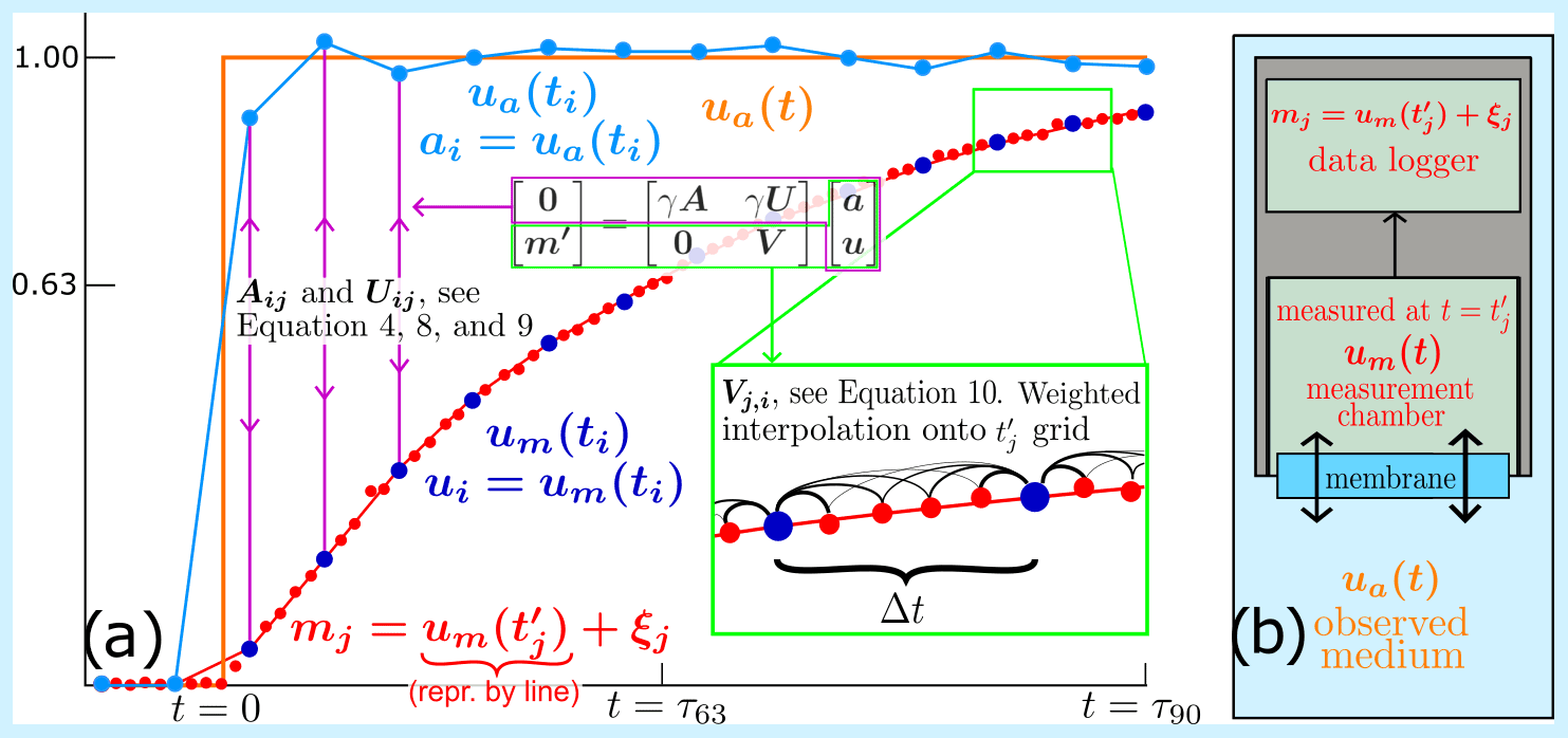
Figure 1(a) Schematic representation of Eqs. (3)–(10) showing the relationship between the measurements (mj, red dots), modeled measurements (red line), and de-convolution process for a step change in ambient property (ua orange line) lasting 2 e-foldings (τ63) of the growth-law equation. Thickness of lines in zoomed inlet indicates weighting during re-sampling onto tj grid. (b) Schematic representation of EB sensor (grey box) during operation and physical location of the different properties in Eqs. (1)–(10). Note that in this schematic we follow the assumptions of linearity in between the model points um(ti) (and not the “true” concentration within the measuring chamber).
We discretize Eq. (1), using a time-symmetric numerical derivative operator (e.g., Chung, 2010):
We have used the following short-hand to simplify notation: um(ti)=ui and ua(ti)=ai. Here ti is an evenly sampled grid of times and is the sample spacing. We refer to ti as model time, and for simplicity we assume that this is on a regular grid Δti=Δt with a constant time step. Note that the growth coefficient ki=k(ti) can vary as a function of time.
We assume that sensor measurements mj of the quantity um(t) obtained at times (see Fig. 1) have additive independently distributed zero-mean Gaussian random noise:
where with the variance of each measurement, which in practical applications can be estimated directly from the data or by using a known sensor accuracy. The is the measurement time, which refers to the points in time where measurements are obtained. Coupling between um(ti) and measurements mj is obtained through gridded re-sampling. Note that the measurement time steps do not need to be regularly spaced, nor coincide with the model times ti.
To reliably estimate ua(t), we need to regularize the solution by assuming some kind of smoothness for this function. A common a priori assumption in this situation is to assume small second derivatives of ua(t), corresponding to the second-order Tikhonov regularization scheme (Tikhonov and Arsenin, 1977). Although this provides acceptable solutions, the choice of the regularization parameter (i.e., adjusting the amount of regularization applied) is not particularly intuitive. Since our method is intended for a variety of domains where validation can be challenging, we have chosen to employ a different regularization method, where the regularization parameter relates directly to simple real-world characteristics and the ability of the instrument to resolve the ambient environment.
Model sparsity regularization (see e.g., Hastie et al., 2015) provides an intuitive model regularization by assuming that the observed quantity can be thoroughly explained by a reduced number of samples in some domain. In our case, we have used time domain sparsity, which translates to setting the number of model time (ti) steps N smaller than the number of measurement time () steps M. The a priori assumption we make to achieve this is that the observed quantity can only change with a time step of
and change piece-wise linearly between these points. Using this approach, an optimal regularization parameter becomes the lowest Δt at which the observed quantity can change significantly. This means that choosing the regularization parameter can be done based on domain-specific knowledge or scientific requirements for temporal resolution, within the limitations posed by the ill-posed nature of the problem and sensor performance.
We can now express the theory, relationship between the measurements and the theory, and the smoothness assumption in matrix form as follows.
Here, contains the standard deviation normalized measurements and and the discretized concentrations ai=ua(ti) and ui=um(ti) (see Eq. 2). N is the number of model grid points i, and M is the number of measurements mj. and express the growth-law relationship between discretized ai and ui as given in Eq. (2). The matrix handles the regularization and the relationship between measurements and the discretized model of um(t). The constant is a numerically large weighting constant (we used , where σs is the smallest σ in m′), which ensures that when solving this linear equation, the solution of the growth-law equation will have more weight than the measurements. In other words, the solution satisfies the growth-law equation nearly exactly, while the measurements are allowed to deviate from the model according to measurement uncertainty. Estimates are insensitive to the exact choice of γ as long as it is large enough to disallow large errors in the growth-law equation solution (which is why it is balanced by σ).
The definitions of the matrices are as follows, where ki is the growth coefficient:
In matrix U we also need to express the time derivative of um(t) and consider edge effects.
The matrix relates concentration ui to measurements of this concentration mj (see Fig. 1 and Eqs. 2 and 3). We use a weighted linear interpolation between grid points ti when assigning measurements to the model:
where Δt is the model time step and regularization parameter (see Eq. 4). It is now possible to obtain a maximum a posteriori estimate of ua(t) and um(t) by solving for the least-squares solution to matrix Eq. (5):
The vector contains the maximum a posteriori estimate of vectors a and u. The matrix G is described in Eqs. (5)–(9). The estimate of ua(t) is the primary interest; however, the solution also produces an estimate of um(t). This can be a useful side product for detecting outliers from fit residuals or other issues with the measurements (as shown in the field experiment).
Equation (10) allows the estimate to also be negative, which can be unwanted if the observed quantity is known positive. In such cases, it is possible to apply a non-negativity constraint using a non-negative least-squares solver (Lawson and Hanson, 1995).
As the uncertainties of measurements are already included in the theory matrix G, the a posteriori uncertainty of the solution is contained in the covariance matrix ΣMAP, which can be obtained as follows:
This essentially achieves a mapping of data errors into model errors, including the prior assumption of smoothness.
The quality of the solution relies on an appropriate choice of regularization parameter Δt and noise/uncertainty in the measurements, but also on the ratio between the RT of the sensor and variance in the property of interest. We develop this further through an application of the theory in a simulation experiment.
2.1 Simulation and Δt determination
To test the numerical validity of our method and develop a regularization parameter selection tool, we used a toy model. This gives us the possibility to prove that the method gives well-behaved, consistent solutions as we know the correct results and control all input variables.
We defined the simulated concentration ua(t) (see also Fig. 1) as a step-wise change in partial pressure:
where units for time and partial pressure are arbitrary. While this is not a realistic scenario encountered under field conditions, step-change simulations are a conventional calibration. It is also the most challenging scenario for testing our method, since it directly violates our smoothness assumption.
The measurement chamber partial pressure um(t) was simulated with a dense grid using a closed-form solution of Eq. (1) from ua(t) and a growth coefficient k=0.1 (τ63=10). A simulated set of measurements mj was then obtained by sampling from um(t) and adding Gaussian noise (see Eq. 3). We assume that measurement errors are proportional to um(t) (measurement uncertainty increases with increasing concentration) in addition to a constant noise floor term, providing a standard deviation for each measurement given by
We used ϵ=0.01 and σ0=0.001 (0.001 + 1 % uncertainty).
As A, U, and m′ of the matrix equation (Eq. 6) are now known, only the regularization parameter Δt in V (Eq. 9) needs to be defined to obtain the gridded estimate of time and RT-corrected measurements (i.e., and ) for the simulated model. For solutions regularized through smoothing, a well-regularized solution captures a balance between smoothness and model fit residuals. Or in more practical terms, the provided solutions are sharp enough so critical information is not lost (i.e., detection of short-term signal fluctuations is not removed by smoothing integration), but with reasonable noise and uncertainty estimates. We have chosen a heuristic approach to this optimization problem, by applying the L-curve criterion (see Hansen, 2001). Statistical methods based on Bayesian probability (Ando, 2010), such as the Bayesian information criterion, were also tested with similar results. We chose to apply the L-curve criterion due to its robustness and ability to intuitively display the effect the regularization parameter has on the solution, which we believe is an advantage in practical applications of our method.
In our case, the L-curve criterion involves calculating a norm Es, which measures how noisy the estimate is and a norm Em, which measures how large the fit residual is (i.e., an estimate of how well the model describes the measurements). These norms are calculated for a set of different regularization parameters, which are compared in a log-log plot (see Fig. 2a) where the data points align to trace a curve that resembles the letter “L”. The under-regularized (or too noisy) solutions are found in the upper left corner where perturbation errors dominate. The over-regularized (or over-smoothed) solutions are located in the lower right corner, where regularization errors dominate. Good regularization parameters are located in the middle of the bend or kink of the L, where smoothness and sharpness are well balanced, limiting both noise and fit residuals.
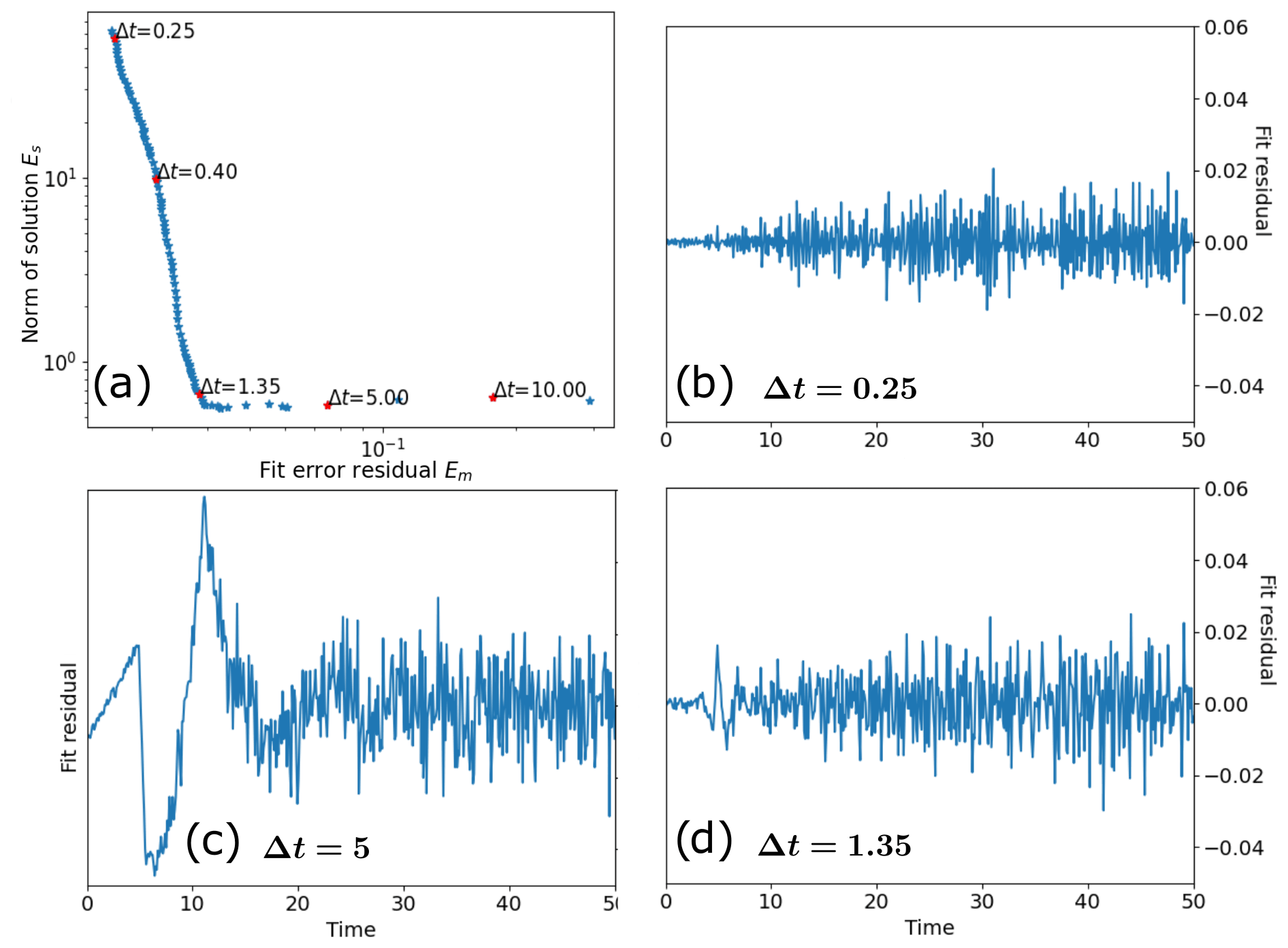
Figure 2(a) L curve for sweep of different Δt values for estimated property (RT correction) of simulated measurements given by . On the y axis, Es is the noise in the data given by the step difference between adjacent data points, which is high for models that are too complex (lower higher number of data points) in the model. The x axis is the fit error residual Em, which shows how well the results (the uas) explain the measurements m. The latter is high for too sparse models (high low number of data points). Panels (b), (c), and (d) show fit residuals for each point in measurement time using Δt=0.25 (b), Δt=5 (c), and Δt=1.35.
We have used the first-order differences of the maximum a posteriori solution as the norm measuring solution noise:
and to approximate the fit residual norm, we use
where mj is the measurement of the quantity um(t):
which comes directly from the least-squares solution (Eq. 10) of matrix Eq. (6), where
corresponds to Vji (see Eq. 9) but without scaling for measurement error standard deviation. In essence, is the best-fit model for the measured quantity um(t) obtained using linear interpolation in time from the least-squares estimates in vector . Note that our definition of Es is not normalized with the number of model points (N), implying a slight favoring of less complex solution (it is possible to normalize with N−1 and M in Es and Em, resulting in slightly more complex solutions in the bend of the L).
We calculated a set of estimates using a wide range of Δt and produced the L curve in Fig. 2a using our norm and fit residual definitions (Eqs. 14 and 15). We plotted estimates of ua(ti) from mj using three different values of the Δts shown in this L curve to inspect an over-regularized, under-regularized, and well-regularized solution. The error estimate, given as a 95 % confidence interval (2σ uncertainty), is obtained from the diagonal terms of the upper left quadrant of the covariance matrix (the quadrant concerning [a,a]; see Eq. 11) using the simulated measurement uncertainties as input variance (which are proportional to um(t) except an offset σ0, Eq. 13). The solution in Fig. 3a resulted from a low Δt=0.25 (upper left in the L curve in Fig. 2a) and is under-regularized and too noisy. The solution has small fit residuals (Fig. 2b), since the high resolution enables the model to represent almost instantaneous changes. Figure 3b shows an over-regularized solution, with a high Δt=5 (lower right in the L curve, Fig. 2a). In this scenario, the noise is minimal; however, the coarse resolution of the model gives poor fit with the signal. This can be clearly seen in Fig. 2c as a spike in the fit residuals at the location of the step change (t=5) where the model is unable to represent the process that produced our measurements due to the poor resolution. Choosing Δt=1.35, located in the bending point of the L in Fig. 2a, provides a well-regularized solution with good balance between noise and model fit residuals. Since we assume that the property of interest changes linearly between our model points, a small irregularity in the model fit residuals also remains at the step here (Fig. 2d) due to the model's inability to capture the high-frequency components of the step function. In practice, the fit residual irregularity arises due to the discrepancy between and mj at the step change (the effect is illustrated in Fig. 1). Nonetheless, with Δt=1.35 the step change is well represented within the limits of the resolution provided by the model assumption without very eye-catching fit residuals, nor unreasonable noise amplification (Fig. 2d).
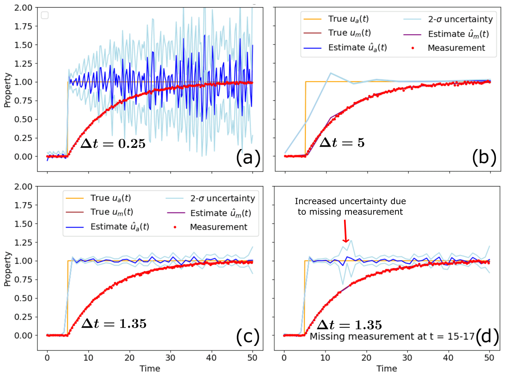
Figure 3Estimated property using simulated data and different regularization parameters (time intervals). The simulated measurements are shown with red points, and the estimated property is shown with a blue line with 2-σ uncertainty indicated with a light blue line. Panel (a) shows a high-temporal-resolution estimate, which is very noisy, due to the ill-posed nature of the deconvolution problem; (b) shows an estimate with a too low temporal resolution, which fails to capture the sharp transition at t=5; and (c) shows a good balance between estimation errors and time resolution. Panel (d) shows estimated property for a simulated dataset with missing measurements between t=15–17, which results in an increased error around the missing measurements for the estimated quantity. Error estimates are given as 95 % confidence intervals.
Using Δt=1.35, we can also inspect how a well-regularized solution is affected by edges and missing measurements (shown in Fig. 3d). The missing measurements resulted in an increased uncertainty in the region where there are no measurements, but the maximum a posteriori estimate still provided a reasonable solution. Uncertainties grow near the edges of the measurement as expected, since there are no measurements before or after the edges which contain information about ua(t).
Choosing the best Δt is a pragmatic task, where the L-curve criterion is a useful guideline. The kink in the L curve can be chosen manually through visual inspection or automatically by identifying the point of maximum curvature. We numerically approximated the maximum curvature location using a spline parameterization of the L curve (method described in Appendix A) to find Δt=1.35. Estimating Δt using the L-curve criterion gives a solution with a numerically optimal compromise (according to our definitions of Es and Em) between noise and information about variability. Increasing or decreasing Δt slightly can be justified in instances where scientific hypotheses require interpretation of very rapid variability or where model fit residuals suggest too crude model complexity for crucial parts of the time series. Nonetheless, if no regularization parameters Δt satisfying the scientific requirements are found in relative proximity of the bend of the “L”, this could indicate that the measurement device is unable to resolve the phenomenon of interest due to low accuracy and/or a too convoluted signal.
Even though the step function is an unrealistic scenario in a practical application, it is likely that the variability of a measured property can change considerably within a single time series. Since the L-curve criterion provides a Δt which is a compromise between error amplification and model fit residuals, this can result in a model complexity which is too crude to resolve important high-variability sections of the data. In this case, inspection of model fit residuals can identify sections of the dataset with too low complexity. Generally, the model fit residuals should be roughly normally distributed and should not have strong irregularities or systematic patterns. Too low complexity causes residual spikes, as shown in the simulation experiment. By identifying such sections in the dataset, considerations can be made, for instance by cautionary data interpretation. Alternatively, it is possible to manually increase model complexity for the whole or certain parts of the time series (by splitting the time series) to reduce the fit residuals in these regions.
We evaluated our proposed technique in a controlled laboratory experiment using a Contros HydroC CH4 EB methane sensor by exposing the sensor to step changes (similar to the numerical experiment) in concentration. We connected the instrument to an airtight water tank (12.9 L) with a small headspace (∼0.25 L) via hoses where water was pumped at 6.25 L min−1 and kept at constant temperature (22 ∘C) (see setup in Appendix B). The setup first ran for 2 h to ensure stable temperature and flow. In this period, the sampling rate was 60 s, while it was changed to 2 s for the rest of the experiment to provide high measurement resolution for the step changes.
Four step changes (two up and two down) were approximated by opening the lid and adding 0.2 L of either methane-enriched or ultrapure water. The RT of the sensor was determined to 23 min at 22 ∘C (k=0.000725 s−1) prior to the experiment following standard calibration procedure of the sensor, and parameters affecting membrane permeation were controlled (i.e., water flow rate over membrane surface and water temperature). Running a calibrated sensor in a controlled environment assuming random errors, we chose to use signal noise as the basis for measurement uncertainty (rather than as stated in the instrument data sheet). This was estimated using the standard deviation of the single point finite differences in the measurement data.
The first 2 h had lower noise due to the reduced sampling rate and hence longer internal averaging period, but noise was otherwise constant and unrelated to the measured concentration. We therefore used two separate σ values (measurement uncertainty): one for the first 2 h and one for the latter part of the measurement period. Δt was determined to 179 s using the automatic Δt selection based on the L-curve criterion (see Appendix A). This also gave well-confined fit residuals, with a difference in signal noise at around 7000 s due to the change in input noise (caused by changes in sampling rate from 60 to 2 s after 2 h, Fig. 4a and b).
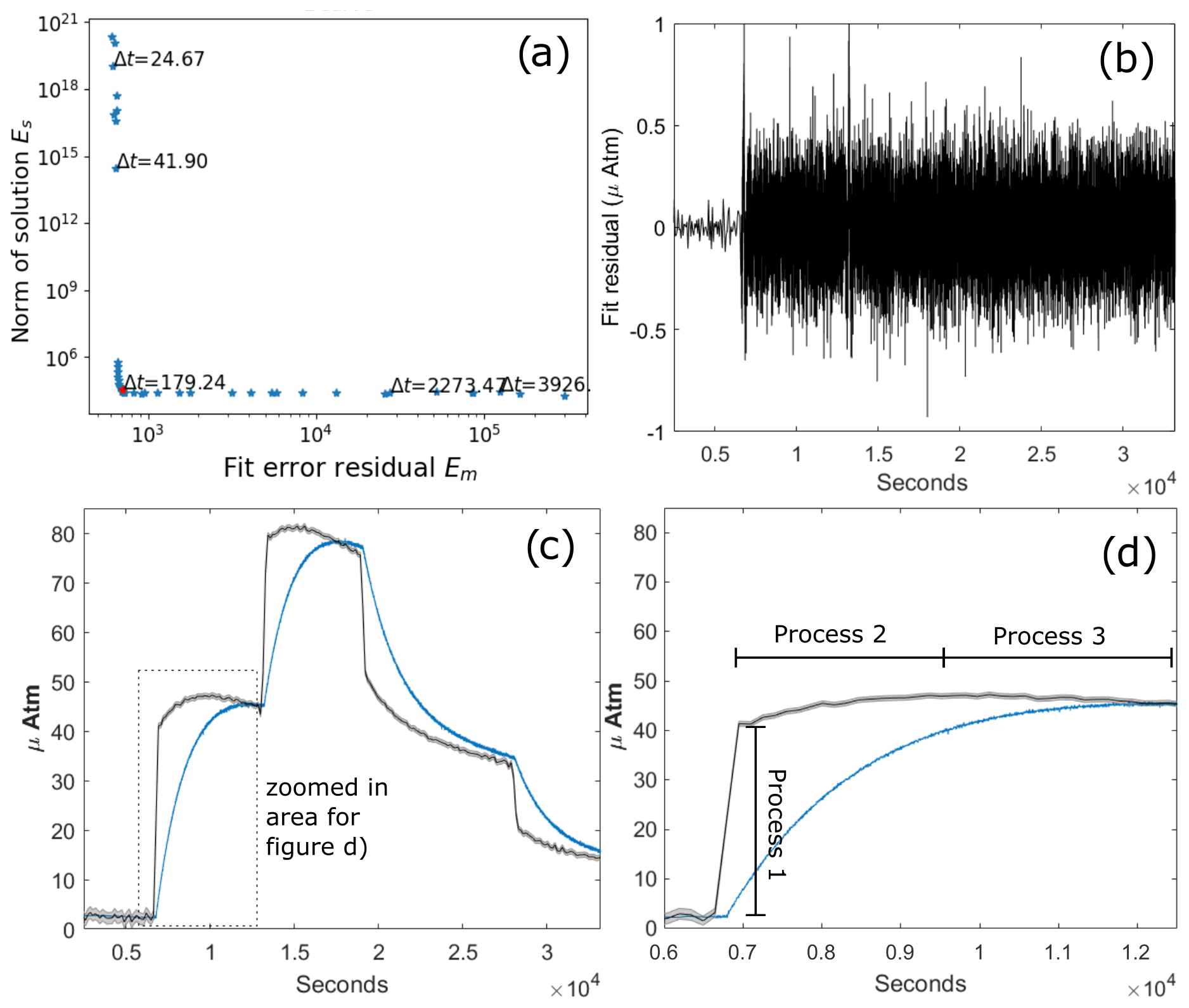
Figure 4(a) L curve for sweep of different Δt values for estimated RT-corrected EB sensor data. The y axis, Es, is the noise in the data given by the step difference between adjacent data points, which is high for models that are too complex (lower higher number of data points) in the model. The x axis is the fit error residual, , which shows how well the best-fit model explains the measurements. (b) Fit residuals (black line) for each point in measurement time using Δt=179 s. Panel (c) shows the result of the deconvolution (black line), uncertainty estimate (grey shading), and raw EB sensor data (blue line). Panel (d) is a zoomed-in version of (c) with area specified in (c).
At the first step change, the RT-corrected concentration rapidly increased from around 2.6 to ∼41 µAtm (Fig. 4c and d). This was followed by a slower increase taking place over around 30 min up to ∼47 µAtm and then a slow decrease for another 30 min down to ∼45 µAtm before the next step change. The following step increase and subsequent two step decreases followed the same pattern, which can be explained by three processes indicated in Fig. 4d. The first rapid increase (process 1) results from the initial turbulent mixing caused by the abrupt addition of methane-enriched water to the tank. This is followed by a slower diffusive mixing phase occurring after the water has settled (process 2). While these processes are occurring, there is also a gradual diffusion of methane to the headspace, which is shown as decreasing concentrations in approximately the last half of the plateau periods (process 3). As expected, this decrease was faster for higher concentrations, due to the larger concentration gradients across the water–headspace interface. The step decreases behave consistently with the step increases, although processes 2 and 3 become indiscernible since they both act towards decreasing the concentration.
Estimated uncertainty of the RT-corrected data averaged 0.64 µAtm (95 % confidence), which is roughly double the raw data noise of 0.29 µAtm. Due to the long concentration plateaus, the balanced Δt lies in a quite strongly regularized solution. Nonetheless, the de-convolved instrument data give a considerably better representation of the step changes with a relatively small uncertainty estimate and reveal known features of the experiment setup (processes 1–3 in Fig. 4d), which is obscured in the convolved data.
Continued evaluation of our proposed technique was applied under more challenging conditions in a field-based study using simultaneous data from two different methane sensors towed over an intense seabed methane seep site offshore west Spitsbergen (Jansson et al., 2019). A slow-response EB Contros HISEM CH4 and a fast-response membrane inlet laser spectrometer (MILS) DRB sensor (Grilli et al., 2018) were mounted on a metal frame and dragged at various heights over the seabed (∼20–300 m) at 0.4–1.1 m s−1 in an area with many hydro-acoustically mapped methane seeps. The rapid and large variability in methane concentration, direct comparison with the DRB sensor, and particularly high RT of the EB sensor in cold water made this an ideal test scenario for field-based applications.
4.1 Growth coefficient and measurement uncertainty
We determined the growth coefficient k (or the inverse, the τ63) for the EB sensor prior to the field experiment (see Appendix C) to be s−1 (τ63=1740 s) at 25 ∘C. Taking the temperature dependency for the permeability of the polydimethylsiloxane sensor membranes into account (Robb, 1968), we found the following relationship for k:
where s−1 is k at temperature T=0 ∘C and ( s−1 for water temperature ∘C in the field experiment). We did not take the RT of the DRB sensor into account in the comparison, since its τ63 was negligible ( s at 25 ∘C) compared to the EB sensor.
The measurement uncertainty (σj in Eq. 13) was set to either the estimated raw data noise or to the stated sensor accuracy after equilibrium is achieved, depending on which of these parameters was higher. The EB accuracy is stated to 3 % using the ISO 5725-1 definition of accuracy, which involves both random and systematic errors. High concentrations during the field experiment made the 3 % sensor accuracy our main input parameter for measurement uncertainty. It is worth noting that this uncertainty regards the gas detection occurring within the measurement chamber and not potential errors caused by other factors such as imperfections with the membrane or pump operation.
4.2 Δt determination
We produced an L curve from a set of estimates of ua(t) with Δt values ranging from 10 to 550 s (Fig. 5a). Using a polynomial spline to approximate the maximum curvature point (see Appendix A), we found the optimal Δt to be 55 s, which is in good agreement with our visual inspection of the L curve. Upon inspection of the fit residual plot (Fig. 5b), we observed large spikes at several time points, meaning that the model failed to describe the transformation between the measurements mj and the RT-corrected estimate ua(ti). Inspection of raw data (red line in Fig. 5b) uncovered sharp signatures in the measured dissolved concentration at these instances – too sharp to be a real signal (as these should have been convolved by the instrumental function). We concluded that there was an unidentified problem with the EB sensor system at these instances, most likely related to power draw, pump failure, or other instrumental artifacts. Removing these problematic sections and re-doing the estimates provided an L curve with an unchanged maximum curvature location. We therefore kept using Δt=55 s in the final deconvolution, which now gave a solution with approximately Gaussian distributed fit residuals without spikes (Fig. 5d), meaning that we have a self-consistent and valid solution.
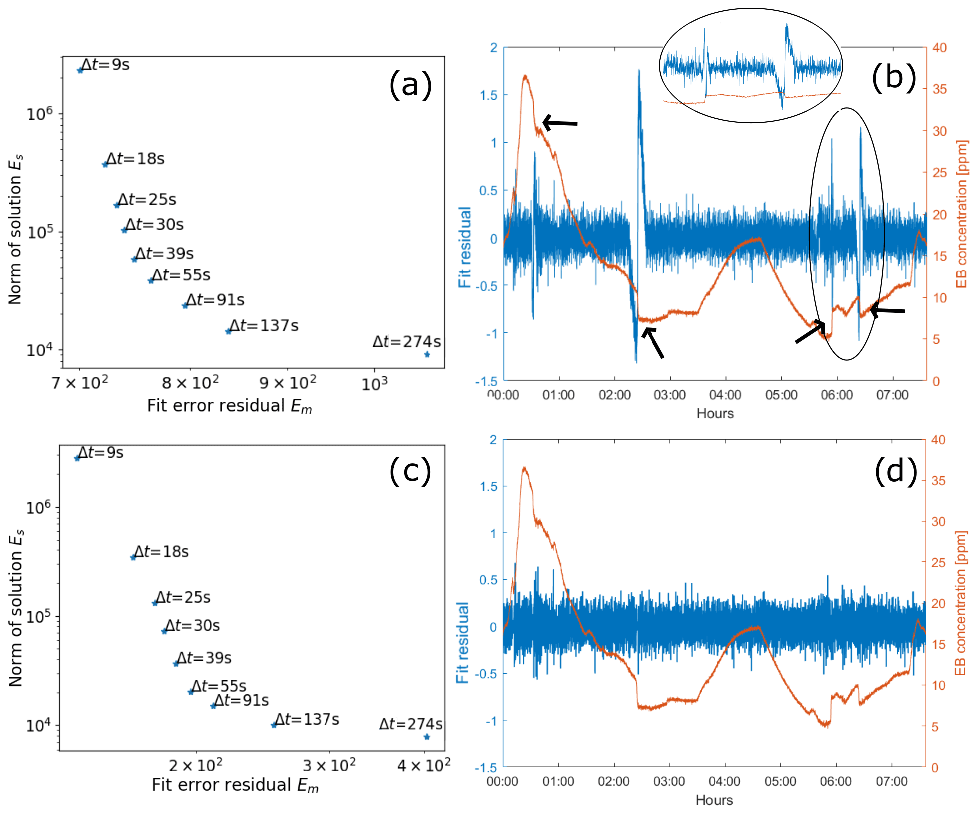
Figure 5(a) L curve for sweep of different Δt values for estimated RT-corrected EB sensor data. The y axis, Es, is the noise in the data given by the step difference between adjacent data points, which is high for models that are too complex (lower higher number of data points) in the model. The x axis is the fit error residual, , which shows how well the best fit model explains the measurements. (b) Fit residuals (blue line) for each point in measurement time using Δt=55 s and raw EB sensor data (red line). Residual spikes attributed to a malfunctioning of the EB sensor are indicated by the black arrows (and zoom in oval inlet). Panels (c) and (d) show the results from the same analysis as (a) and (b), but on the dataset where the problematic regions defined in (b) were removed.
4.3 Sensor data comparison
The comparison between DRB, EB, and RT-corrected EB sensor data collected during the transect offshore west Spitsbergen is shown in Fig. 6. We used the coefficient of determination (R2) and the mean absolute error to compare the datasets (having already validated the method numerically and in the laboratory test).
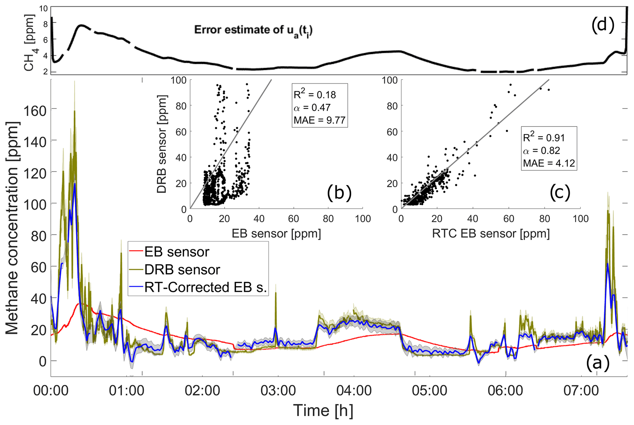
Figure 6(a) Field data from the DRB (yellow), EB (red), and RT-corrected EB (blue) sensors. Panels (b) and (c) show direct comparison between DRB and the EB sensor data. Coefficient of determination (R2), mean absolute error (MAE), and slope angle (α) are given for comparison between the DRB sensor data and either raw (b) or RT-corrected (c) EB sensor data. Panel (d) shows the error estimate of the RT-corrected signal, ua(ti), as 2 standard deviations.
The untreated EB sensor data clearly show how the convolution creates a strong hysteresis effect and makes the sensor unable to directly detect rapid changes in methane concentration. This results in a low coefficient of determination (R2=0.18), high mean absolute error (MAE=9.77 ppm), and flat slope angle (α=0.47) when compared to DRB data (Fig. 6a and b). RT-corrected EB data, on the other hand, match the DRB data well (R2=0.91, MAE=4.1 and α=0.82, Fig. 6a and c), showing that high-resolution data were indeed convolved in the EB data and that our method managed to retrieve them successfully.
The high R2 of the RT-corrected data confirms that the EB sensor captured most of the variability in dissolved methane; however, there is a slight bias in the differences between the two datasets (α=0.82). Inspecting the absolute differences reveals that the RT-corrected EB data have more moderate concentrations during periods of very strong variability. This can partly be explained by the inherent smoothing of a sparse model (for larger Δt). In theory, increasing the model complexity (reducing Δt) should return a slope closer to 1 and reduce differences. However, our attempt at decreasing Δt for achieving this did not improve the slope, but increased the noise as expected. The flat slope could also at least partly originate from the previously problematic sections (spikes in Fig. 5) in the EB sensor data (arrows in Fig. 5b). Even though we ignored the data at these intervals, the offset in absolute concentration still affects our end estimate. Another explanation could be an overestimation of the k of the EB sensor in the laboratory procedure prior to the field campaign. Indeed, when using a lower k, e.g., corresponding to τ63=3600 s (keeping Δt=55 s), which matches better with calibration results for similar sensors, the slope goes to 1 and differences are evenly distributed between high and low methane concentrations. The small slope offset could also be a combined effect of the above-iterated reasons.
Using the framework of inverse theory allows us to model error behavior by calculating the covariance matrix ΣMAP (see Eq. 11 and Appendix D), enabling a comparison of the uncertainty estimates of the two sensors (shaded regions in Fig. 6). For the DRB sensor data, we used the stated 12 % accuracy as the uncertainty estimate (Grilli et al., 2018). For the RT-corrected EB data, we used the 95 % confidence of the deconvoluted estimate using input measurement uncertainty, resulting in a median uncertainty range of 22 %. Linearly interpolating the RT-corrected EB data onto DRB data time and taking the mutual error bounds into account, the two datasets agree within the uncertainties 92 % of the time. This is despite the lower resolution of the RT-corrected data and other potential error sources (some described above), and we consider this a successful result.
The DRB data have a lower median relative (%) uncertainty estimate, but to compare these relative uncertainty estimates directly can be slightly misleading as the relative uncertainty estimate of the RT-corrected data varies in time (Fig. 6d). This is due to the EB sensor convolution occurring prior to the time when the actual measurement (including measurement uncertainty) takes place (see Fig. 1b). Since input measurement uncertainty mostly follows 3 % of measured (already convolved) value, the uncertainty estimate becomes a function of the EB raw data. Consequently, due to the raw data hysteresis, the uncertainty becomes lower for increasing concentrations compared to decreasing concentrations, and vice versa. We can observe this at ∼00:15 and ∼07:15 LT, when the RT-corrected concentration increases dramatically, but the uncertainty estimate is still relatively small (Fig. 6a and d). On the other hand, between 04:40 and 05:30 LT, the RT-corrected concentration data are relatively low and constant, but the uncertainty estimate is large and shrinks slowly due to the slow decrease in um(t). Comparing the error bounds of the datasets using the relative uncertainty is therefore a simplification because of the raw-data-inherited RT-corrected uncertainty estimate. Overall, this adversely affects the relative uncertainty estimate of the RT-corrected dataset, since high error bounds inherited from the raw-data hysteresis during decreasing concentrations are divided by RT-corrected low concentration values, which results in high relative uncertainties. A more narrowly defined (if possible) input uncertainty estimate for the EB sensor could help constrain this uncertainty.
We presented and successfully applied a new RT-correction algorithm for membrane-based sensors through a deconvolution of the growth-law equation using the framework of statistical inverse problems. The method requires few and well-defined input parameters, allows the user to identify measurement issues, models error propagation, and uses a regularization parameter which relates directly to the resolution of the response-time-corrected data. Functionality testing was done using both a laboratory and a field experiment. Results from the laboratory experiment uncovered features of the experimental setup which were obscured by convolution in the raw data, and the field experiment demonstrated the robustness of the algorithm under challenging environmental conditions. In both tests, the sensors' ability to describe rapid variability was significantly improved, and better constraints on input uncertainty and response time are areas which can potentially further enhance results.
This method and validation experiments using the Contros/HISEM sensors uncover a new set of applications for these and similar sensors, such as ship-based profiling/towing and monitoring of highly dynamic domains. Conventional EB sensors are also more abundant and affordable compared to more specialized equipment, increasing the availability and possibilities for scientists requiring high-resolution data to solve their research questions. Additionally, we believe this deconvolution method could be applicable to other measurement techniques as well, where diffusion processes hamper response time.
Even though Δt sometimes can be chosen purely based on the practical problem at hand, we also want to provide a more rigorous way of choosing Δt applicable at any circumstance. There are several ways to approach this problem (see e.g., Ando, 2010), but we have used the L-curve criterion. Even though Δt can be chosen through visual inspection of the L curve, we also provide the option of automatic Δt selection to further simplify and provide more robustness to the methodology. This is done by finding the point of maximum curvature in the L curve, which corresponds to the kink of the L. We do this by fitting a fourth degree smoothness regularized cubic spline to a sweep of a given number of solutions estimated using evenly distributed Δt values between a Δt corresponding to one-half of the measurement time step up to a maximum of 2000 model points and a Δt corresponding to a 10-point model grid. A Δt located in the bend of the L can then be found by using the derivatives of the polynomials in the spline and maximizing the curvature given by
where and are the splines of Em and Es and using Lagrangian differential notation. Smoothing is done by including the second derivatives weighted by a smoothing parameter in the minimization criteria of the spline fit.
One issue that arose during development of the automatic Δt selection algorithm was that it was applied to data from a toy model where we tried to estimate a step change in property (Fig. 3 in paper). This is of course an unrealistic situation to encounter in any field application of a real instrument and is also in violation of any smoothness assumption we make on the solution. More specifically, we assume that changes in ua(t) can only occur following a piece-wise linear model with a time resolution of Δt, which is violated in the case of an instantaneous step change. The L-curve criterion will nonetheless give us the best possible approximation we can get to the most likely solution of our problem. However, the fit residuals between and mj will be dependent on the match or mismatch between the time steps in ua(ti) (with resolution defined by Δt) and the time when the instantaneous step change occurs. In essence, if there is a good match between the model time steps and the instantaneous step change, the model will be able to produce lower fit residual and vice versa. The result of this is that the spline fit can, depending on the location of the knots, produce local points with very high curvature which are not located in the kink of the L. We counteracted this effect when using the toy model data by doing a simple running mean and sorting of the noise and fit residual data for the solutions produced during the Δt sweep, which resulted in consistent results. In a real-world application where there is constant but less abrupt variability, this should not be an issue, but we kept the running mean filter to increase the robustness of this approach. We also compared the automated model selection based on the L-curve criterion as iterated herein with model selection based on the Bayesian information criterion (see e.g., Ando, 2010), which gave similar results. Nonetheless, it is recommended that the ability to visually inspect the L-curve is exploited, to ensure the automatic selection has worked as expected.
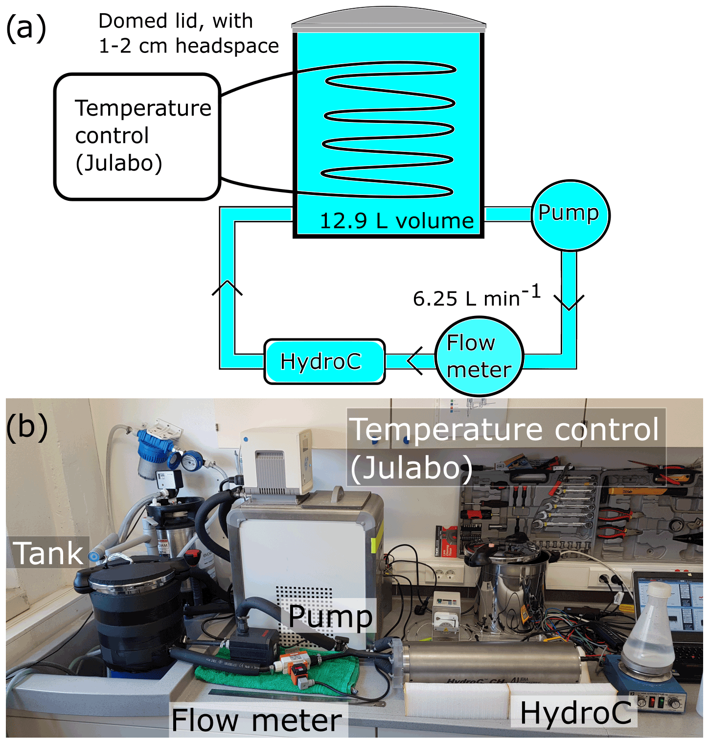
Figure B1(a) Schematic representation of the experiment setup and (b) picture of the experiment setup. The tank had an airtight dome-shaped lid with a small headspace (∼0.3 L) and was 27.5 cm high and 24.5 cm diameter. Room temperature was controlled and kept constant.
To apply our methodology to the EB field sensor dataset and compare with the DRB data, the sensor growth coefficients k (or τ63) are required. Since no calibration data were available on location, we estimated k directly prior to the field campaign by placing both instruments in a freshwater-filled container (25 L, 25 ∘C), where ∼500 mL of methane enriched water was added instantaneously to simulate a step change in concentration. The water was continuously mixed using the two submersible pumps provided by the instruments and corrected for degassing to the atmosphere. With this setup, k was estimated to s−1 (τ63=1740 s) for the EB sensor and s−1 (τ63=13 s) for the DRB sensor.
Water temperature and salinity have a direct impact on k for both these sensors due to changes in gas permeation of the membrane (Robb, 1968). This makes k a function of time in a field experiment where these properties are varying. Based on laboratory testing on the permeation efficiency of the polydimethylsiloxane (PDMS) membranes used in both sensors (see Grilli et al., 2018) we found that k increased linearly with temperature following
where k0 is k at T=0 ∘C and αk is a constant individually determined for each sensor. The effect of salinity was negligible at the low water temperatures at our field study site. To keep the RT of the fast-response sensor as low as possible during the field campaign, we increased the total gas flow in the DRB sensor, thereby counteracting some of the loss in responsiveness due to lower water temperature. The water temperature range during the field study was 4.0–6.4 ∘C, which gave a k between and s−1 (τ63=2285–2381 s) for the EB sensor and between 0.120 and 0.125 s−1 (τ63=8.0–8.3 s) for the DRB sensor, taking increased gas flow into account.
Figure D1 shows the covariance matrix from the field experiment (ΣMAP as calculated by Eq. 11). The upper left quadrant of Fig. D1 concerns the [a,a] covariances, and the diagonal elements are the model uncertainty estimates. The other quadrants concern the [a,u], [u,a], and [u,u] covariances. Note that the color scales in Fig. D1 are set to be small to increase the contrast of the plot.
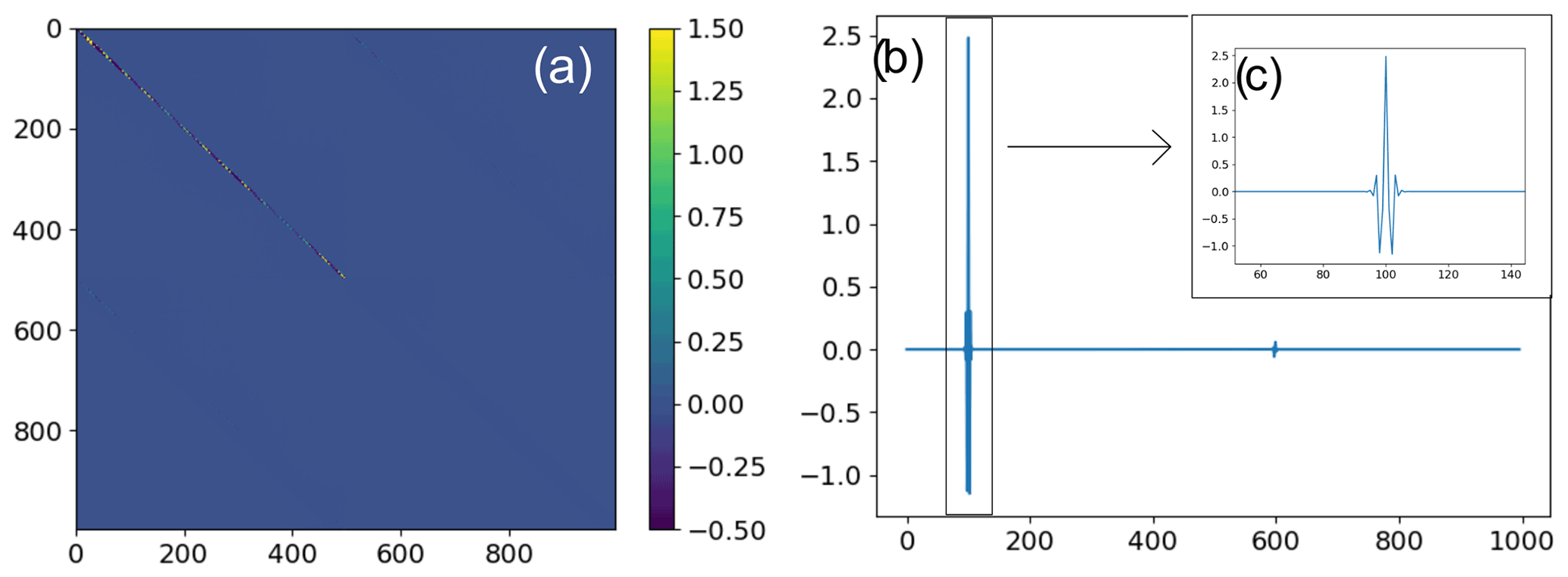
Figure D1(a) Covariance matrix from response time correction of field experiment data. The [a,a] covariance is shown in the upper left quadrant, and the lower left and upper right quadrants with very faint but visible diagonals show the [a,u] and [u,a] covariance matrices (b) Row 100 of the covariance matrix and (c) a zoomed-in excerpt of row 100 of the covariance matrix (approximate region indicated by the square in c).
The fluctuations on each side of the diagonal elements (non-diagonal elements) in row 100 (see Fig. D1b and c) show that there is auto-correlation in the error estimates of a. This is expected since the elements in a are constructed from a set of linear combinations of the elements of m′ and also, being well confined in time, of little concern (see e.g., Aster et al., 2019).
All data and code presented in this paper can be obtained here: https://github.com/KnutOlaD/Deconv_code_data (last access: 2 August 2022).
Writing, original draft preparation, and method and software development were done by KOD and JV. Data were curated by KOD and RG. Investigation and formal analysis were done by KOD, JV, and RG. Visualization was done by KOD. The project was administrated and supervised by KOD, RG, JT, and BF. Resources and funding were acquired by RG, JT, and BF. All authors contributed to reviewing and editing the manuscript.
The contact author has declared that none of the authors has any competing interests.
Publisher's note: Copernicus Publications remains neutral with regard to jurisdictional claims in published maps and institutional affiliations.
The research leading to these results has received funding from the European Commission's Seventh Framework Programmes ERC-2011-AdG under grant agreement no. 291062 (ERC ICE&LASERS), the ERC-2015-PoC under grant agreement no. 713619 (ERC OCEAN-IDs), and the Agence National de Recherche (ANR SWIS) under grant agreement no. ANR-18-CE04-0003-01. Additional funding support was provided by SATT Linksium of Grenoble, France (maturation project SubOcean CM2015/07/18). This study is a part of CAGE (Centre for Arctic Gas Hydrate, Environment and Climate), Norwegian Research Council (grant no. 223259). We thank the crew of R/V Helmer Hanssen, Pär Jansson for initial discussions of the manuscript idea, Snorre Haugstulen Olsen for input on the automatic Δt selection, and Nick Warner for proofreading a previous version of the paper and general feedback on the content of the manuscript.
This research has been supported by the European Research Council, FP7 Ideas: European Research Council (grant no. ICE&LASERS (291062)), the H2020 European Research Council (grant no. OCEAN-IDs – OCEAN in-situ Isotope and Dissolved gas sensing (713619)), the Agence Nationale de la Recherche (grant no. ANR-18-CE04-0003-01), the Société d'Accélération du Transfert de Technologies (grant no. Maturation project SubOcean CM2015/07/18), and the Norges Forskningsråd (grant no. 223259).
This paper was edited by Takehiko Satoh and reviewed by two anonymous referees.
Ando, T.: Bayesian Model Selection and Statistical Modeling, 1st edn., Chapman and Hall/CRC, https://doi.org/10.1201/EBK1439836149, 2010. a
Aster, R. C., Borchers, B., and Thurber, C. H.: Parameter estimation and inverse problems, 3rd edn., Elsevier, 2019. a, b
Atamanchuk, D., Tengberg, A., Aleynik, D., Fietzek, P., Shitashima, K., Lichtschlag, A., Hall, P. O. J., and Stahl, H.: Detection of CO2 leakage from a simulated sub-seabed storage site using three different types of pCO2 sensors, Int. J. Greenh. Gas Con., 38, 121–134, https://doi.org/10.1016/j.ijggc.2014.10.021, 2015. a
Bittig, H. C., Fiedler, B., Scholz, R., Krahmann, G., and Körtzinger, A.: Time response of oxygen optodes on profiling platforms and its dependence on flow speed and temperature, Limnol. Oceanogr.-Meth., 12, 617–636, https://doi.org/10.4319/lom.2014.12.617, 2014. a, b
Canning, A. R., Fietzek, P., Rehder, G., and Körtzinger, A.: Technical note: Seamless gas measurements across the land–ocean aquatic continuum – corrections and evaluation of sensor data for CO2, CH4 and O2 from field deployments in contrasting environments, Biogeosciences, 18, 1351–1373, https://doi.org/10.5194/bg-18-1351-2021, 2021. a, b
Chung, T. J.: Derivation of Finite Difference Equations, in: Computational Fluid Dynamics, 2nd edn., Cambridge University Press, 45–62, https://doi.org/10.1017/CBO9780511780066.007, 2010. a
Faïn, X., Chappellaz, J., Rhodes, R. H., Stowasser, C., Blunier, T., McConnell, J. R., Brook, E. J., Preunkert, S., Legrand, M., Debois, T., and Romanini, D.: High resolution measurements of carbon monoxide along a late Holocene Greenland ice core: evidence for in situ production, Clim. Past, 10, 987–1000, https://doi.org/10.5194/cp-10-987-2014, 2014. a
Fiedler, B., Fietzek, P., Vieira, N., Silva, P., Bittig, H. C., and Körtzinger, A.: In Situ CO2 and O2 Measurements on a Profiling Float, J. Atmos. Ocean. Tech., 30, 112–126, https://doi.org/10.1175/JTECH-D-12-00043.1, 2013. a
Grilli, R., Triest, J., Chappellaz, J., Calzas, M., Desbois, T., Jansson, P., Guillerm, C., Ferré, B., Lechevallier, L., Ledoux, V., and Romanini, D.: Sub-Ocean: Subsea Dissolved Methane Measurements Using an Embedded Laser Spectrometer Technology, Environ. Sci. Technol., 52, 10543–10551, https://doi.org/10.1021/acs.est.7b06171, 2018. a, b, c, d
Hansen, P.: The L-Curve and Its Use in the Numerical Treatment of Inverse Problems, vol. 4, WIT press, 119–142, 2001. a
Hastie, T., Tibshirani, R., and Wainwright, M.: Statistical Learning with Sparsity: The Lasso and Generalizations, 1st edn., Taylor & Francis, 2015. a
Jansson, P., Triest, J., Grilli, R., Ferré, B., Silyakova, A., Mienert, J., and Chappellaz, J.: High-resolution underwater laser spectrometer sensing provides new insights into methane distribution at an Arctic seepage site, Ocean Sci., 15, 1055–1069, https://doi.org/10.5194/os-15-1055-2019, 2019. a
Kaipio, J. and Somersalo, E.: Statistical and computational inverse problems, vol. 160, Springer Science & Business Media, 2006. a
Lawson, C. L. and Hanson, R. J.: Solving least squares problems, SIAM, 1995. a
Miloshevich, L. M., Paukkunen, A., Vömel, H., and Oltmans, S. J.: Development and validation of a time-lag correction for Vaisala radiosonde humidity measurements, J. Atmos. Ocean. Tech., 21, 1305–1327, 2004. a, b, c, d, e
Robb, W. L.: Thin silicone membranes – Their permeation properties and some applications, Ann. NY Acad. Sci., 146, 119–137, https://doi.org/10.1111/j.1749-6632.1968.tb20277.x, 1968. a, b
Tikhonov, A. and Arsenin, V.: Solutions of Ill-Posed Problems, 1st edn., Winston & Sons, Washington, DC, USA, 1977. a, b
- Abstract
- Introduction
- Method
- Laboratory experiment
- Field experiment
- Conclusions
- Appendix A: Automatic Δt selection
- Appendix B: Laboratory setup
- Appendix C: Growth coefficient determination for field experiment
- Appendix D: Covariance matrix from field experiment estimate
- Code and data availability
- Author contributions
- Competing interests
- Disclaimer
- Acknowledgement
- Financial support
- Review statement
- References