Drone-towed controlled-source electromagnetic (CSEM) system for near-surface geophysical prospecting: on instrument noise, temperature drift, transmission frequency, and survey set-up

Drone-borne controlled-source electromagnetic (CSEM) systems combine the mobility of airborne systems with the high subsurface resolution in ground systems. As such, drone-borne systems are beneficial at sites with poor accessibility and in areas where high resolution is needed, e.g. for archaeological or subsurface pollution investigations. However, drone-borne CSEM systems are associated with challenges, which are not observed to the same degree in airborne or ground surveys. In this paper, we explore some of these challenges based on an example of a new drone-towed CSEM system. The system deploys a multi-frequency broadband electromagnetic sensor (GEM-2 uncrewed aerial vehicle, UAV), which is towed 6 m below a drone in a towing-bird configuration together with a NovAtel GNSS–IMU (global navigation satellite system–inertial measurement unit) unit, enabling centimetre-level position precision and orientation. The results of a number of controlled tests of the system are presented together with data from an initial survey at Falster (Denmark), including temperature drift, altitude vs. signal, survey mode signal dependency, and the effect of frequency choice on noise. The test results reveal the most critical issues for our system and issues that are likely encountered in similar drone-towed CSEM set-ups. We find that small altitude variations (± 0.5 m) along our flight paths drastically change the signal, and a local height vs. signal correlation is needed to correct near-surface drone-towed CSEM data. The highest measured impact was −46.2 ppm cm⁻¹ for a transmission frequency of 91 kHz. We also observe a significant increase in the standard deviation of the noise level up to 500 % when going from one transmission frequency to five. We recommend not to use more than three transmission frequencies, and the lowest transmission frequencies should be as high as the application allows it. Finally, we find a strong temperature dependency (up to 32.2 $\mathrm{ppm}{}^{\circ }{\mathrm{C}}^{-\mathrm{1}}$), which is not accounted for in the instrumentation.

1 Introduction

Small uncrewed aerial vehicles (UAVs; drones) are becoming increasingly more popular survey platforms (instrumental carriers) for geophysical and archaeological prospecting, and a vast number of applied geophysical studies use different types of sensors as part of drone-borne systems. Among others, drones are used as an instrumental carrier for ground-penetration-radar studies (Altdorff et al., 2014), gamma-ray studies (Mochizuki et al., 2017), thermal investigations (Poirier et al., 2013; Petzke et al., 2013), lidar (Risbøl and Gustavsen, 2018), and magnetic investigations (Lev and Arie, 2011; Petzke et al., 2013; Døssing et al., 2021; Schmidt and Coolen, 2021; Kolster et al., 2022). In general, electromagnetic induction methods are among the most commonly used techniques for mineral exploration but are, to our knowledge, not commonly used as a drone-borne system. Some studies working with drone-borne electromagnetic systems (Karaoulis et al., 2020; Mitsuhata et al., 2022) use, for example, the GEM-2 UAV from Geophex to measure the electromagnetic response from the subsurface. One alternative method to this approach is the semi-airborne solution described in Kotowski et al. (2022), where the transmitter is placed on the ground instead of transporting the transmitter together with the receiver on the drone. As drone-borne solutions are still advancing, we here strive to further push the investigation of drone-borne solutions with electromagnetic sensors.

Controlled-source electromagnetic (CSEM) systems and techniques are popular in both airborne and handheld applications, while drone-borne CSEM systems are, as mentioned before, less common. Large airborne CSEM systems, typically by helicopter (heliborne), can cover large areas quickly and effectively and are mainly associated with large-scale geophysical prospecting (Siemon et al., 2009). Handheld applications are typically associated with small-scale geophysical prospecting using a smaller instrument coil size, which – combined with a low operation height – produces high spatial resolution of near-surface targets. The modern CSEM sensor systems, for both heliborne and handheld applications, are complex and highly suited for each specific application with different pros and cons. While handheld versions lack mobility (wetlands, lakes, and overgrown areas are difficult to map), heliborne systems are highly mobile but are also more costly and provide lower spatial resolution due to increased survey height.

A handheld instrument mounted on drones can improve mobility and increase the range of access with the same spatial resolution as handheld surveying at an affordable price. However, the drone platform introduces several technical challenges, particularly related to the drone's electromagnetic noise and the undesired movement of the sensors during flight, both of which can reduce the quality of the data if not accounted for. The electromagnetic noise from the drone becomes an issue when the drone and the CSEM sensor are too close, since the sensor is unable to separate the electromagnetic response of the subsurface from the electromagnetic noise from the drone. One possible solution for reducing noise is a towed bird system, which is often used for airborne systems that deploy electromagnetically sensitive sensors. A towed bird system is essentially a wire configuration that connects the instrumentation with the instrument carrier (drone or helicopter), which allows the instrumentation to be towed at a certain distance underneath the platform during flight. A towed bird configuration, however, introduces undesirable oscillations and movements of the instrument, something that needs to be precisely monitored and recorded by GNSS (global navigation satellite system) and IMU (inertial measurement unit) sensors on board the bird (Kolster et al., 2022).

When dealing with CSEM instrumentations, we operate with a transmitting and a receiving coil. A theoretical description of the coils and the electromagnetic field has been given in various textbooks (e.g. Ward and Hohmann, 1988; Telford et al., 1990; Kaufman et al., 1983; Everett, 2013), which explain several techniques and geometrical configurations for a set of coils that can be employed in geophysical prospecting. In this context, Ward and Hohmann (1988) present a beneficial description of the electromagnetic behaviour for finite sources over a layered half-space and provide expressions for coils separated by a distance above a layered subsurface. The expressions by Ward and Hohmann (1988) also include the height above the surface, which changes during flight for a drone-borne system. In addition, the towed bird oscillates in pitch, heading, and roll, providing an individual height change for the receiving and transmitting coils. This influences the readings significantly when flying close to a surface.

Here, we focus on a bistatic multi-frequency configuration. We present our findings for a drone-towed CSEM system and highlight some precautions that should be taken when collecting data. We use the controlled-source electromagnetic induction sensor GEM-2 UAV from Geophex (Lerssi et al., 2016). Our approach is tuned to achieve the highest possible quality of data for near-surface archaeological prospecting. Still, our results can also be used for other targets in the subsurface. We present tests concerned with instrument noise, temperature drift, transmission frequency, and survey set-up. These tests enable us to clarify – and correct for – some of the visual irregularities in our drone data. We include our recommendations for producing high data quality for drone-borne CSEM systems.

2 Method

As part of the method, we introduce the CSEM sensor in Sect. 2.1, followed by the description of our drone-towed system in Sect. 2.2. When we combine the CSEM sensor with the drone-towed system, we refer to it as a drone-towed CSEM system. Section 2.3 describes some tests conducted with the CSEM sensor alone as well as tests conducted with the drone-towed CSEM system. The purpose of the tests is to clarify some of the unwanted features in the CSEM survey data. Finally, in Sect. 2.4, we describe how we typically plan and execute surveys with the drone-towed CSEM system, and as a case study, we explain how it was used in a test site near Virket at Falster, Denmark.

2.1 CSEM sensor (GEM-2 UAV)

Documentation of the GEM-2 UAV is sparse. However, the instrument shares most of its features with the handheld version of the GEM-2 for ground surveys (Lerssi et al., 2016), which has been shown to be useful for archaeological prospecting (Tang et al., 2018). Other CSEM sensors of interest for near-surface prospecting include the Dualem-1S, EM38, and Profiler 400-EMP (Abdu et al., 2007; Bjella et al., 2010). Among these and other instruments, the GEM-2 UAV was selected because it is lightweight and has a multi-frequency setting.

The GEM-2 UAV can operate at up to 10 frequencies between 25 Hz and 96 kHz simultaneously, and it weighs approximately 3 kg, excluding a battery and positioning system. Operating the GEM-2 UAV requires a suited battery, a GNSS antenna, and the WinGEM software installed on a laptop. In terms of power consumption, the GEM-2 UAV requires 18–28 V and consumes 20 W during surveying (transmission mode) and less than 2.5 W during standby mode. The instrument has an input plug for GNSS antenna connection, with a baud rate of 9600 and word format of “8 data bits”, “1 stop bit”, and “no” hardware flow control (9600, 8, 1, N).

The GEM-2 UAV is shaped like a ski with a receiving (Rx) and transmitting (Tx) coil located at each end, 1.6 m apart. This is named a “bistatic” configuration, which allows us to survey in different “modes”, where P and T mode indicate whether the ski is aligned or transverse with the survey direction, respectively, and the vertical and horizontal coplanar mode indicates whether the coils are levelled vertically or horizontally. The latter should not be confused with the horizontal or vertical dipole–dipole configuration, which also deals with coil configurations but refers to the coil's magnetic or electrical dipole moment. Our tests and surveys only operate the sensor in the horizontal coplanar mode. Nonetheless, when flying with the sensor, we expect a little oscillation and rotation, which has an impact on the assumption of a perfect horizontal coplanar mode.

Before starting a survey with the GEM-2 UAV, it needs to be initialised and set to log the data. This is achieved by connecting to the GEM-2 UAV's control unit, which also provides the option of choosing the transmission frequencies and the length of the median filter, located on top of the ski. Once these operating options have been chosen, the GEM-2 UAV's transmission mode is switched on, and data logging starts.

The raw data extracted from the GEM-2 UAV are in-phase and quadrature responses in parts per million (ppm). These in-phase and quadrature data are the real and imaginary part of the ratio between the magnetic intensity fields from the receiving coil (H_s) and transmitting coil (H_p). A discussion of the different ways of expressing this field ratio is outside the scope of this paper, but it is useful for the subsequent discussion to state it as described in Ward and Hohmann (1988):

$$\begin{array}{}\text{(1)}& {\displaystyle \frac{H_{\mathrm{s}}}{H_{\mathrm{p}}}}=r^{\mathrm{2}}\underset{\mathrm{0}}{\overset{\mathrm{\infty }}{\int }}{\displaystyle \frac{u-\mathit{\lambda }}{u+\mathit{\lambda }}}\mathit{\lambda }{e}^{-\mathrm{2}\mathit{\lambda }h}{J}_{\mathrm{1}}\left(\mathit{\lambda }r\right)\mathrm{d}\mathit{\lambda },\end{array}$$

where r is the distance between coils; h is the height above the surface; J₁ is the Bessel function of the first order; λ is called the separation constant ($\mathit{\lambda }=\sqrt{(k_x^{\mathrm{2}}+k_y^{\mathrm{2}})}$); and u is the modified wavenumber ($u=\sqrt{({\mathit{\lambda }}^{\mathrm{2}}-k^{\mathrm{2}})}$), where k is the wavenumber. The wavenumber is assumed to be iωμσ in our application for low-frequency domains, where μ is magnetic permeability, μ₀ is the free-space permeability, σ is the electrical conductivity, and ω is the angular frequency with the relation ω=2πf to the transmission frequency f.

The expression in Eq. (1) is frequently used in airborne EM applications in which the survey height is an essential parameter. The expression also enables us to convert in-phase and quadrature parts-per-million values into the apparent electrical conductivity and magnetic susceptibility, respectively (Huang and Fraser, 2000, 2001, 2002). It should be noted that the susceptibility is most prominent in the in-phase response at lower transmission frequencies (Won and Huang, 2004); i.e. it is valuable, for near-surface applications, to have both the quadrature response from high transmission frequencies and the in-phase response from low transmission frequencies as this enables us to precisely calculate susceptibility and conductivity for near-surface targets.

The default median filter uses three data points, which means it will output data at sampling $\frac{\text{sampling\hspace{0.17em} rate}}{\text{median\hspace{0.17em} filter}}=\frac{\mathrm{25}}{\mathrm{3}}$ Hz. However, there is plenty of space on the 32 Gbit SD card to store raw, unfiltered data, even for a full day of surveying, thereby allowing the user to conduct the preferred filtering of the data instead. In addition to the actual data output, the GEM-2 UAV conveniently also stores a parts-per-million value for the local power line amplitude, which indicates how affected the data are by the local power grid.

The sensor can use up to 10 transmitted frequencies. Still, the factory only recommends using five or fewer transmitted frequencies for which the skin depth $D=\frac{\mathrm{1}}{\sqrt{\mathit{\pi }\mathit{\mu }\mathit{\sigma }f}}$ is convenient in a simple estimation of the depth of penetration (Huang, 2005).

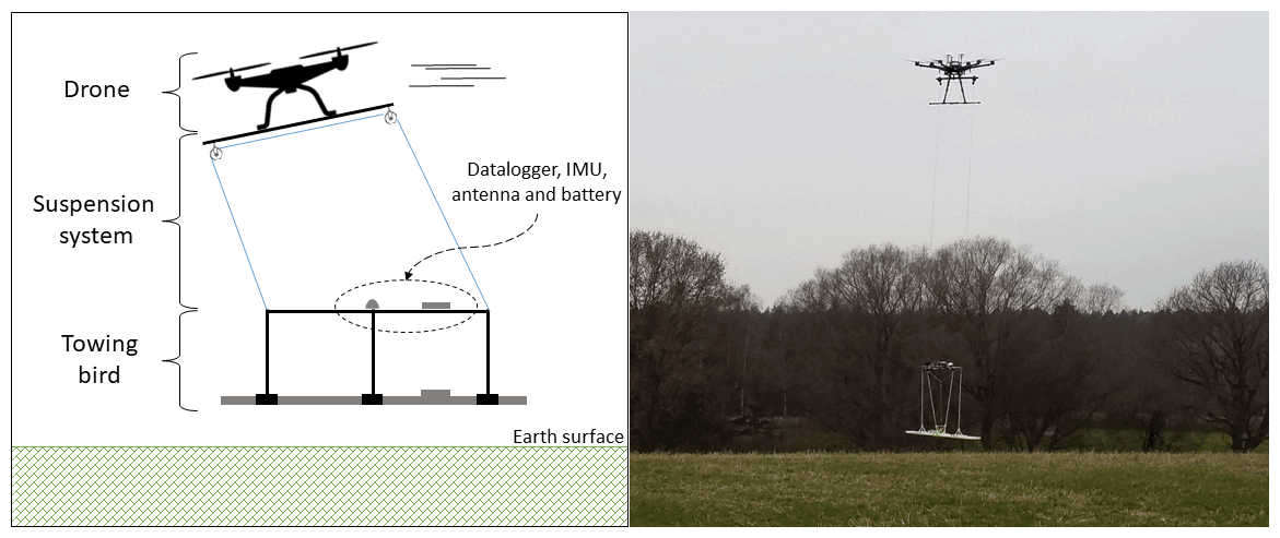
Figure 1 An illustration on the left of the drone set-up and a picture from a field survey in Falster, Denmark.

2.2 Drone-towed system

The drone-towed system consists of three main parts: the drone; the suspension system; and the towing bird set-up, which also houses the GEM-2 UAV sensor (Fig. 1).

For the survey drone, we used the off-the-shelf DJI Matrice 600 Pro, which has a maximum recommended payload of 15.5 kg and a flight time of approximately 20 min with the survey set-up. The Matrice 600 Pro is equipped with real-time kinematic positioning (RTK), which includes ground station communication with the drone by radio link.

The suspension system is the Technical University of Denmark (DTU)-patented sensor suspension system (, ), in which a pulley system keeps the towing bird levelled and its direction constant during surveying. Based on the knowledge gained, which we discuss later, the length of the suspension system was set to 6 m.

The towed bird consists of a semi-rigid frame, which carries the CSEM sensor and a battery as well as an external, high-precision NovAtel GNSS–IMU and logging device for precise positioning and 3D altitude information. The frame is constructed out of non-conductive fibreglass and 3D-printed plastic, which allows us to separate the GNSS–IMU, logging device, and battery from the CSEM sensor, thereby reducing the electromagnetic noise. The 3D-printed parts of the frame ensure a flexible design, which proved to be extremely valuable during the initial developmental phase. The 3D-printed set-up also allows the CSEM sensor to be easily replaced if a superior sensor becomes available. The total weight of the towing frame, battery, high-precision GNSS–IMU, and logging device is 2 kg; combined with the 3 kg CSEM sensor, the precisely positioned drone-towed CSEM system weighs 5 kg in total.

2.3 Tests

Following completion of the drone-towed CSEM system and initial flight tests, we encountered some irregularities in the data, which had not previously been identified for the handheld applications. In order to investigate the cause of these irregularities, we performed a series of tests on both the CSEM sensor itself and on the drone-towed CSEM system as a whole.

Test 1:

P and T mode. A handheld walking survey was performed across a metal target with a strong electromagnetic response. The test was repeated twice while pointing the instrument in different directions, first in P mode, pointing the GEM-2 UAV ski parallel to the survey direction, and next in T mode, pointing the GEM-2 UAV perpendicular to the survey direction. The goal of the P- and T-mode test was to evaluate the sensitivity of the sensor and the difference in the positioning of a small target with precisely known positioning.

Test 2:

temperature drift. In this test, we compared the ambient temperature with changes in output parts-per-million values from three transmitted frequencies. The measurements were conducted in a quiet electromagnetic environment, in which the instrument was subjected to temperature changes by exposing it to direct sunlight or by shading it from sunlight. The duration of the test was 1.5 h, during which the instrument did not move and was not manipulated in any way. The purpose of the temperature drift test was to evaluate the sensitivity of the sensor to temperature changes.

Test 3:

height above surface correlation – static. We tested the change in parts-per-million values for different heights above the surface. In a series of static tests, the instrument measured for at least 3 min at a fixed XY position but at different heights for every 3 min. This was achieved by suspending the instrument by two wires between two trees. By pulling the wires, the height above the surface could be adjusted. The purpose of this test was to provide direct information about the height versus signal correlation as we expected the drone to be unable to maintain a constant (within centimetres) flight altitude throughout a survey.

Test 4:

noise effect of multiple transmitted frequencies. Initial tests with the GEM-2 UAV indicated a significant correlation between noise and the number of transmitted frequencies. The goal of this test was, therefore, to illustrate the dependency of instrumentation noise on the number of transmitted frequencies. The test consisted of five independent sub-tests, each of which had the following transmission frequencies:

• 1.

  475 Hz alone;

• 2.

  91 275 Hz alone;

• 3.

  475 and 91 275 Hz together;

• 4.

  475, 23 175, 45 875, 68 575, and 91 275 Hz together;

• 5.

  475, 10 575, 20 675, 30 725, 40 825, 50 925, 61 025, 71 075, 81 175, and 91 275 Hz together.

For all measurements, the instrument was placed in a fixed position 1 m above the surface and in an area with low electromagnetic noise. We evaluated the noise by calculating the standard deviation for a low transmitted frequency (475 Hz) and a high transmitted frequency (91 275 Hz) from each of these independent sub-tests. Each of the tests lasted for more than 3 min.

Test 5:

noise effect of spacing between transmitted frequencies. Another noise investigation test was performed; this time it was designed to investigate how the separation between two transmitted frequencies changes the instrumentation noise. We paired up two transmitted frequencies and calculated the standard deviation for 475 and 91 275 Hz. The pairs we used were as follows:

• the standard deviation of the transmitted frequency 475 Hz using the pairs 475 and 91 275 Hz, 475 and 23 175 Hz, 475 and 45 875 Hz, and 475 and 68 575 Hz;

• the standard deviation of the transmitted frequency 91 275 Hz using the pairs 91 275 and 475 Hz, 91 275 and 23 175 Hz, 91 275 and 45 875 Hz, and 91 275 and 68 575 Hz.

Test 6:

noise from drone. The aim of this final test was to evaluate the noise from the drone in a convincing but straightforward way to find a threshold at which point the drone is no longer visible in the output parts-per-million values. We conducted the test for a transmitted frequency of 475 and 93 075 Hz individually. The test was conducted by hovering the drone at a certain altitude for at least 1 min and evaluating the standard deviation of the data.

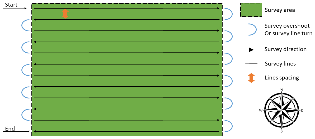
Figure 2 A sketch of a survey design where line spacing, survey heights, and length of survey overshoot are some of the parameters that need to be considered when doing a CSEM survey.

2.4 Drone-towed CSEM study at Falster, Denmark

A drone-towed CSEM test survey was carried out at Falster, Denmark. The study site is close to the town of Virket, which has received a lot of attention recently since what is believed to be the biggest Viking fortress discovered in Denmark is located there (TV2Øst, 2020). The total area of the site is 78 000 m², of which half is a golf course, and the other half is a field. The area has a 5 m embankment on three sides. Planning and conducting a survey requires a lot of thought, but the structure and terminology are very similar for ground and airborne surveys. Figure 2 below is an illustration of a simple survey design. A similar approach was used for the Falster study.

A drone-borne lidar topography survey was conducted to produce a precise local topography model of the survey area. The topography model was included in the drone flight planning software, UgCS, and the drone was set to fly at an altitude which resulted in a distance between the sensor and the surface of 1 m. The survey line spacing was set to 0.5 m, with a 5 m overshoot at the ends. Based on the outcome of the P-mode versus T-mode test (Test 1), we conducted the Falster survey with a constant heading in T-mode configuration, i.e. the sensor always pointed in the same direction (the CSEM Tx coil, for the given survey, pointed in a north-easterly direction). Since it was being towed 6 m underneath a drone in a suspension system, the sensor was not expected to have a completely straight path, as seen in the ideal case in Fig. 2. Therefore, a lot of effort was put into post-processing the GNSS and IMU positioning information of the system with NovAtel software (NovAtel Inc.). Post-processing enables knowledge of the sensor's positioning and orientation down to the level of centimetres. Data in overshoot, landing, and take-off were removed.

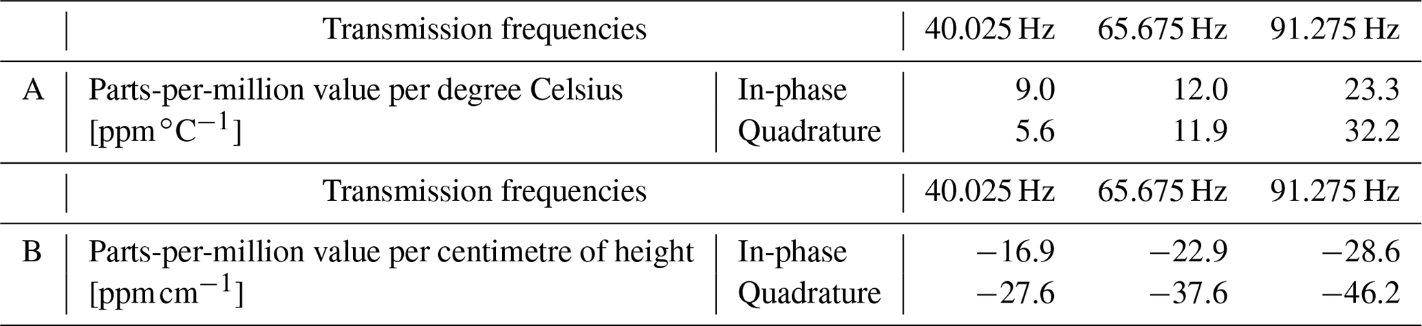
Table 1 (A) The estimated temperature effect on parts-per-million values for 40 025, 65 675, and 91 275 Hz. The unit is parts per million per degree Celsius ($\mathrm{ppm}{}^{\circ }{\mathrm{C}}^{-\mathrm{1}}$), which is calculated from the maximum and minimum values for parts-per-million values and temperature. (B) The slope of the linear fit from Fig. 5.

3 Results

This section uses the raw parts-per-million values from the CSEM sensor. We compare the test results with the standard deviation of the Falster study (Table 1C). The expectation is that the standard deviation of the Falster study will indicate a typical response from the subsurface. It should be noted that similar results concerning the standard deviation of a flight survey were made in previous investigations for a different study site in Denmark (Bjerg et al., 2020). Additionally, Table 1 contains numbers concerning temperature, height above the surface, and the correlation between height and parts-per-million values for the Falster study. The numbers in Table 1 are meant to collect and clarify essential issues of the results.

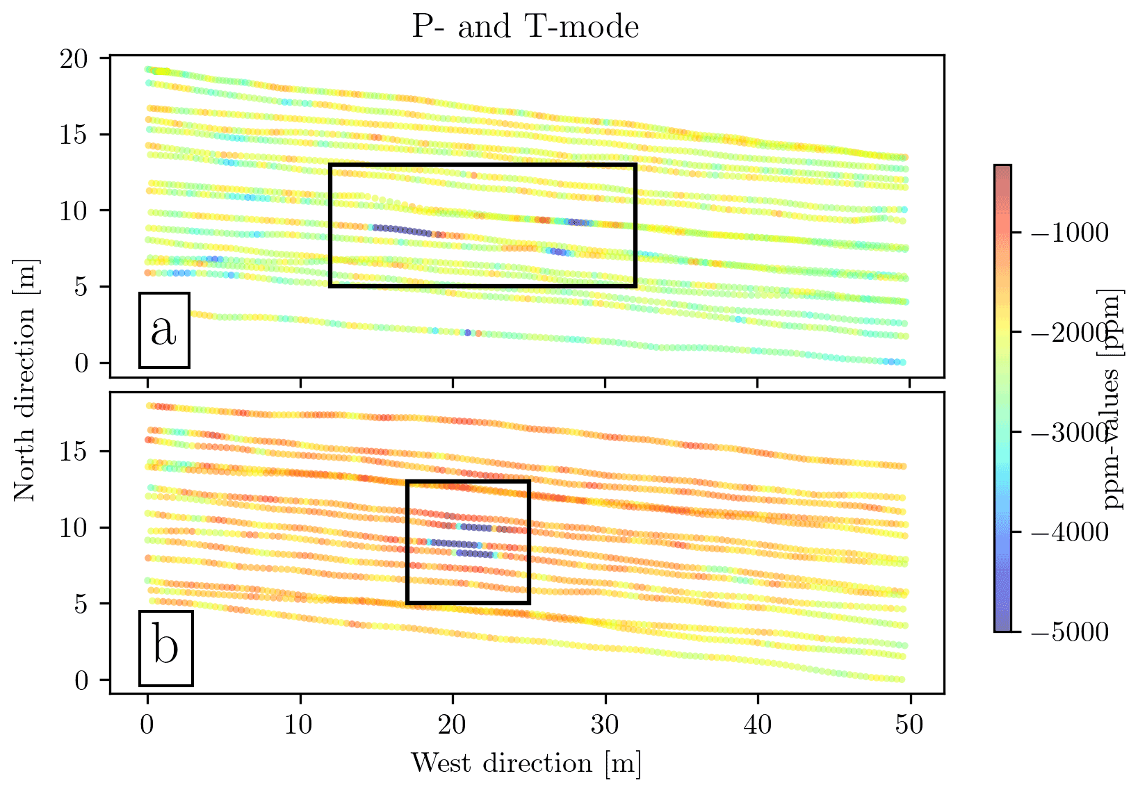
Figure 3 Results of Test 1: (a) P mode and (b) T mode. A heavy metal object is placed in the centre of the survey; the black square encloses the area where it is observed in the data. The object is detected in three survey lines in both the P and T mode. Note that the P mode has a distinctly higher peak anomaly value for the centre survey line compared to the two adjacent lines.

3.1 Test results

Figure 3 shows the measurements from Test 1. The data are the sum of the quadrature response with the transmitted frequencies of 475, 1525, 5325, 18 325, and 63 025 Hz. Figure 3a shows measurements in P mode, while Fig. 3b shows measurements in T mode. The heavy metal object, which is placed in the centre of the survey to show the response in P and T mode, is visible in the form of high peaks in the data for three adjacent survey lines in both modes. A black square encloses the data containing these peaks. Even though we might expect the peaks to be aligned across the survey lines, both P and T mode contain misalignment across adjacent lines. The peak values are shifted along the survey lines by approximately 10 and 1.5 m in P and T mode, respectively; i.e. each data point is shifted by about 5 and 0.75 m forward in the survey direction to align in P and T mode, respectively. If it is assumed that the misalignment is entirely due to a delay in time-stamping, it corresponds to a delay of 0.24 and 2.04 s for P and T mode, respectively, based on an estimated data point shift of 2 and 17 points with the known sampling rate of 8.3 Hz.

Another interesting outcome of the P-mode and T-mode test is the difference in the amplitude of the recorded signal. The target response has a stronger peak value for the adjacent lines when using T mode, which suggests a stronger response from targets across the survey line when surveying in T mode.

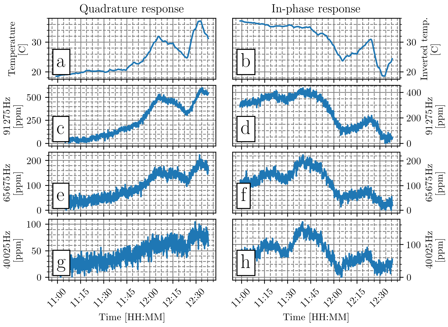
Figure 4 Results of Test 2: a static CSEM versus temperature measurement conducted in a quiet electromagnetic environment. The data are levelled to zero and processed with a median filter. Panels (a) and (b) are the measured temperatures, but (b) is multiplied by −1 to invert the temperature for better comparison with parts-per-million observations for different frequencies in (c) to (h).

The results of the temperature drift Test 2 are visualised in Fig. 4. Figure 4a and b show the temperature and inverse temperature in degrees Celsius, while Fig. 4c–h show the corresponding parts-per-million values for three different transmitted frequencies. A clear correlation is seen between parts-per-million values and temperature. However, the correlation is less pronounced for the lower transmission frequencies. In this connection, the y-axis ranges, which are scaled individually, should be noted. We have calculated an estimated temperature effect per degree (Table 1A), for which we used the difference between the maximum and minimum parts-per-million values and temperatures. We observe that the temperature effect decreases with decreasing transmitting frequencies. Even though the temperature effects from Table 1A at 40 045 Hz appear negligible, the temperature effects are still visible in Fig. 4.

Figure 5 Results of Test 3 (measured parts-per-million values versus instrument altitude). Each measurement is a mean value of 3 min at each altitude. The Pearson correlation coefficient between altitude and parts-per-million values is in the range [−0.98, −0.99].

The results of Test 3 are shown in Fig. 5, in which the dependency between height above ground and the parts-per-million value is demonstrated. The CSEM sensor is recording above the same spot but at 12 different heights between 10 and 130 cm above the surface. The red lines in Fig. 5 represent a linear fit to the data. Note that the fit does not have the same slope or interception with the y axis for any of the frequencies. The slopes of the individual fits are listed in Table 1. We conducted this test at different locations, which produced different slopes and interceptions, but all with a linear trend. Although the linear fit is not a perfect representation of the height dependency, it provides a useful first approximation and indicates the correlation between height above ground and the parts-per-million value.

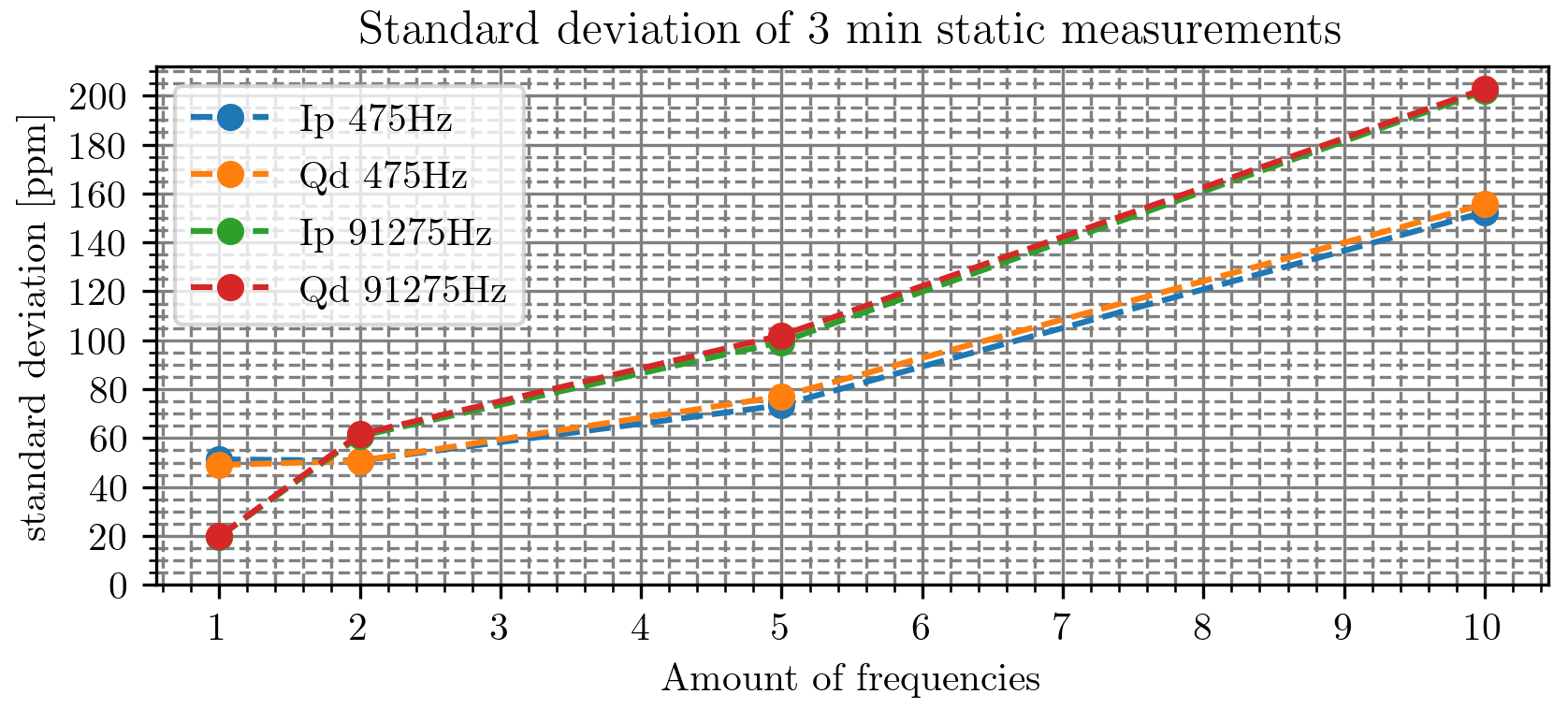
Figure 6 Results of Test 4. The calculated standard deviation for 475 and 91 275 Hz is shown with different numbers of transmitted frequencies. Note that when the number of frequencies equals 1, it is the standard deviation on the frequency itself without any other transmitted frequencies. The additional frequencies between 475 and 91 275 Hz are linearly spaced.

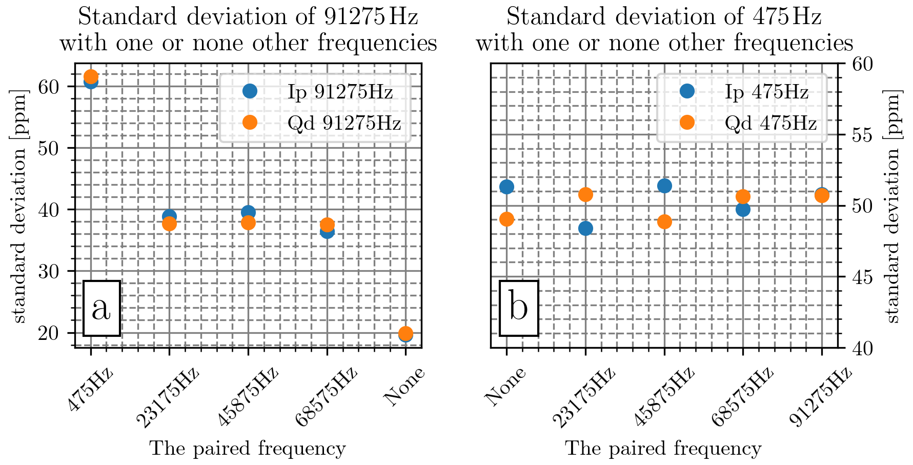
Figure 7 Results of Test 5. The standard deviation is calculated for 91 275 and 475 Hz with one additional transmitted frequency with decreasing spacing. Note that no notable effect is in 475 Hz, while the standard deviation in 91 275 Hz increases with increasing spacing.

In Figs. 6 and 7, we present the results of Tests 4 and 5, which are related to the calculated standard deviation for different combinations of transmitted frequencies and for different spacing between transmitted frequencies. Figure 6 illustrates how the standard deviation is highly dependent on the number of frequencies. The standard deviation for 91 275 Hz with the additional 475 Hz ranges from a standard deviation of ∼ 20 to ∼ 60 Hz, while the effects on 475 Hz having any additional transmission frequency are negligible. Adding, for example, three frequencies between 475 and 91 275 Hz will have an effect on both the 475 and 91 275 Hz frequencies, with the strongest effect at 91 275 Hz (Fig. 6). For five transmitted frequencies, the standard deviation ranges from 73 to 102 Hz, where a standard deviation of 73 Hz is the smallest value for all five transmitted frequencies. As seen in Fig. 7, we further observe that the spacing between the frequencies has a strong effect on the output noise level. This is particularly evident when pairing high frequencies (e.g. 91 275 Hz) with lower frequencies, an effect that was observed to increase as the spacing between the frequencies increased. Here, it may be of value to compare with the standard deviation from the Falster study in Table 1C, in which the noise from 475, 1525, and 5325 Hz is close to 73 Hz, indicating that the noise from the number of frequencies and frequency spacing is the main signal in the Falster study for these frequencies. In contrast, a standard deviation of 478.6 Hz in the quadrature response in the Falster study is a promising signal-to-noise ratio.

Table 2 A collection of values from Test 6. We can read from the numbers that at around 4.2 to 5.2 m, the noise from the drone is no longer visible in the data.

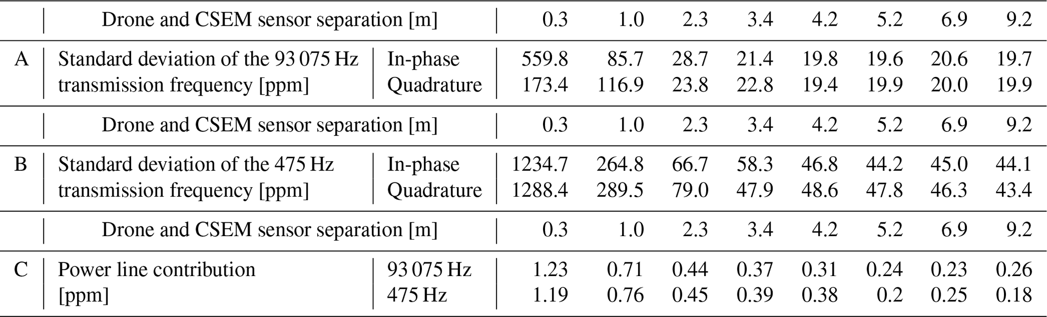
Table 2 lists the results of Test 5, which are related to the noise effect of distance to the drone. The table lists the calculated standard deviation of the parts-per-million values collected with the drone hovering above the CSEM sensor at different altitudes. The effect of the drone is negligible above 5.2 m, while a significant noise effect is observed at shorter distances. At a distance of 0.3 m (i.e. the sensor is mounted on the drone landing gear), the standard deviation increases by a factor 30. This is almost a 3000 % increase in standard deviation compared to the 5.2 m scenario. For the results in the Falster study (see below), we used a distance of 6 m to ensure that the effect from the noise from the drone was negligible.

Figure 8 Falster drone-towed CSEM survey. The survey was carried out in T mode. In (a) quadrature 63 025 Hz is shown, and in (b) in-phase response at 475 Hz for quadrature is shown. The black box outlines the sub-area in Fig. 9.

Figure 9 Close-up picture of a part of the Falster survey data (see black box in Fig. 8). Note the inconsistency in values between adjacent survey lines.

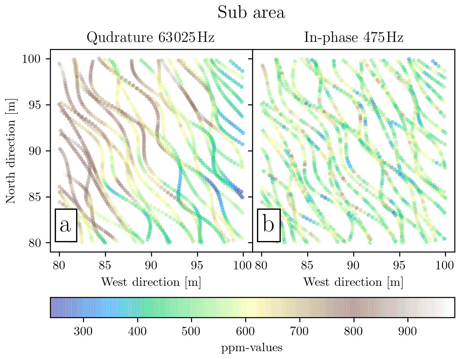
3.2 Drone-towed CSEM study at Falster, Denmark

Figure 8 shows the results of the Falster study made with the drone-towed CSEM. The figure displays the raw response from quadrature at 63 025 Hz in Fig. 8a and in-phase response at 475 Hz in Fig. 8b. From the description in Sect. 2.1 we would expect the response in Fig. 8a to be dominated by conductivity and the response in Fig. 8b to be dominated by susceptibility. The highlighted sub-area in Fig. 8 is enlarged and shown in Fig. 9. Note that the parts-per-million values between the adjacent and overlapping survey lines are generally inconsistent.

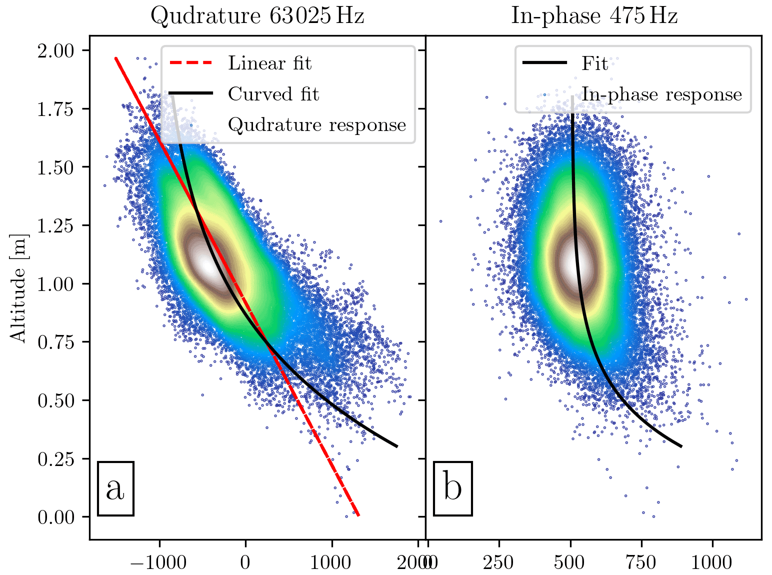
Figure 10 Parts per million versus altitude for the Falster survey data shown as a scatter-density plot. (a) Quadrature response at 63 025 Hz, (b) in-phase response at 475 Hz. We calculated a fit on the form of $a+b\cdot \exp (h\cdot c)$, represented here as the black line. The parameters a, b, and c in the fit can also be found in Table 3. We further calculated the linear fit for the quadrature response (slope of ∼ 14 ppm cm⁻¹, shown with the red line) in order to honour the linear correlation results of the controlled Test 3 in Fig. 5.

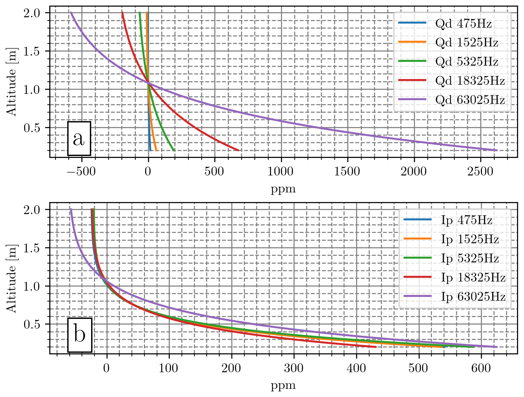
Figure 11 Calculated fits of parts-per-million values vs. altitude for all frequencies of the Falster survey. The parameters a, b, and c are optimised to the smallest least-squares misfit for the equations $a+b\cdot \exp (h\cdot c)$, where h is the altitude. All parameters are listed in Table 3.

Table 3 (A) The calculated standard deviation of the Falster survey. The parameters a, b, and c shown in Fig. 11. Row (B) shows the parameters of the least-squares fit for the quadrature response, and (C) shows the parameters of the least-squares fit for the in-phase response.

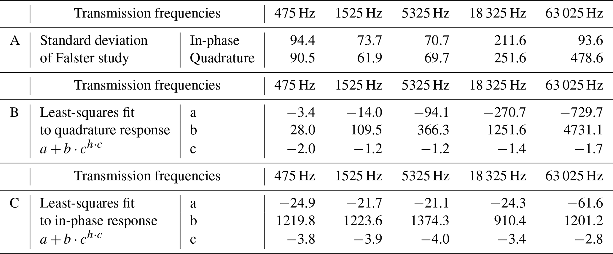
In Fig. 10, we show a scatter-density plot of the raw parts-per-million value vs. altitude for the Falster study. As seen, the majority of the measurements are at 1 m above ground ± 0.5 m. Least-squares fits to the data in Fig. 10 are also shown based on the expression $a+b\cdot \exp (h\cdot c)$, where h is the altitude, and a, b, and c are the optimised parameters. Reasonable fits are observed for both the quadrature and in-phase data. In Fig. 11, we show the fits for all the frequencies. We do not see a perfect linear dependency as we observed in the results of Test 3 (Fig. 5). It is apparent from Fig. 11 that the quadrature responses are very sensitive to altitude change, in particular, at the high frequencies (18 325 and 63 025 Hz), while the in-phase response is generally less affected as soon as the altitude is above 1 m. For the quadrature response at 63 025 Hz, the change from 0.5 to 1.5 m is 1600 ppm, resulting in approximately 16 ppm cm⁻¹, while for the in-phase response at 63 025 Hz, the same change in altitude results in a change in response of 280 ppm. All the estimated parameters and the calculated standard deviation for the Falster survey are listed in Table 3.

Figure 12 Falster survey data before and after altitude correction. (a) Quadrature response at 63 025 Hz, (b) altitude-corrected quadrature response at 63 025 Hz, (c) in-phase response at 475 Hz, (d) altitude-corrected in-phase response at 475 Hz.

Figure 12a and b show the parts-per-million values from the quadrature response at 63 025 Hz and the in-phase response at 475 Hz after correcting for the altitude dependency. The time delay was small, and we found no visible effect by including a delay. Figure 12 can be compared to Fig. 8 as a before-and-after altitude correction. As seen, the altitude-corrected data for the quadrature response (Fig. 12a) are significantly smoother than without the altitude correction (Fig. 8a). Even though the in-phase response at 475 Hz is treated in the same way, we found no visible improvement between Fig. 8b and Fig. 12b. Similar altitude correlation was examined for all data, but the quadrature response at 63 025 Hz was the only one that exhibited an improvement.

4 Discussion

In the paper, we present a drone-towed CSEM system. It is a very adaptable solution that can be used for various applications and is affordable compared to heliborne solutions. We consider the presented wire-based drone-towed CSEM system satisfactory and significantly improved compared to walking surveys for difficult terrain or for areas too large to cover by foot. The system fulfils a new role between heliborne and ground surveys for applications where the heliborne solution is too expensive or impractical. The majority of other existing drone solutions is, to our knowledge, semi-airborne solutions where the transmitter is an integrated part of the drone set-up. Compared to the semi-airborne solution, the presented CSEM solution in this study has the advantage that the transmitter source does not constrain the data collection. The external GNSS–IMU system enables higher precision and time resolution of the position and orientation, which was not available in the GEM-2 UAV instrumentation.

Even though we believe the presented CSEM system has considerable potential, we see possibilities for optimisation in a future version and find it necessary to consider and discuss some of its disadvantages and what could be improved.

The choice of CSEM sensor (i.e. the GEM-2 UAV instrumentation) was limited by the payload capabilities of the available survey drone. A more powerful drone would allow the use of different instrumentation but would also come at the expense of greater noise and higher costs. Ultimately, a light payload increases flight time per battery, which is desirable regardless of the drone. The system presented in this study is based on a towed CSEM sensor. An alternative way of constructing a drone CSEM system is to mount the sensor directly under the drone. However, as seen in Table 1, this would generate between 28 and 8 times more noise in the data. Therefore, based on the results presented here, it is not a question of whether or not to use a towed CSEM system but rather how to overcome the challenges associated with the swaying in a wire-based towing solution.

An alternative to the wire-based towing solution is provided by Karaoulis et al. (2020), who use a rigid towing system and a bistatic sensor system like the GEM-2 UAV from Geophex. Whether a rigid or a wire suspension is most reasonable is difficult to determine without a proper test. A rigid suspension system generates less unwanted swaying but increased noise. The effect of roll, pitch, and heading is the biggest question in our system. While we could not find any direct correlation between roll, pitch, heading, and parts-per-million values, we are confident that changes in these parameters affect our measurements, albeit not as a simple linear correlation. This non-linear behaviour is also demonstrated in Tølbøll and Christensen (2007) as a sensitivity profile in the subsurface.

The roll, pitch, and heading are closely related to the altitude, which currently has the strongest effect on our data, as observed in Test 3 and the Falster study. We observe a clear correlation between the altitude and the parts-per-million value. However, only for the quadrature response at 63 025 Hz does a correction for the altitude significantly improve the data quality (Fig. 12). The altitude is rarely an issue when producing a handheld walking survey because the surveyor can maintain the instrumentation at approximately the same altitude throughout the survey. For heliborne surveys, the altitude is typically included in the processing. Still, the heliborne data – given the significantly higher survey altitude – is less affected by the instrument's orientation (roll, pitch, heading) and altitude. Therefore, it is sufficient to use one collective altitude for the system (like in Eq. 1) and neglect the roll, pitch, and heading changes. However, with a parts-per-million-to-altitude correlation of ∼ 46 ppm cm⁻¹ (Table 1) and an altitude change of ± 0.5 m during a near-surface (∼ 1 m above the surface) drone survey, ignoring these effects becomes problematic. When a drone-towed CSEM sensor system moves close to the surface, any small changes in roll, pitch, and heading will have a stronger effect than in a heliborne system. While it would also be convenient to assume only one altitude measure, it seems insufficient for our application at low altitudes. If we were to analyse this effect numerically, we would need to treat each coil independently and abandon the generally accepted assumption of one altitude for both coils in the instrument (i.e. Eq. 1). Hence, the roll, pitch, and heading effects may explain why we do not observe a linear altitude dependency in the Falster study as observed in the controlled altitude in Test 3.

In Fig. 11b, we observe that the slope of parts-per-million values vs. altitude converges to a similar response with decreasing frequencies. This effect arises from the relation to the wave number described in Won and Huang (2004), implying no dependence on either frequency or conductivity at low transmission frequencies for the in-phase response. It means that the response is mainly real at low frequencies, while the response is primarily complex at high frequencies. These observations become important when deciding on a set of transmission frequencies for a survey; if one wants to estimate both the magnetic susceptibility and the electrical conductivity, it is practical to have at least one high quadrature and one low in-phase frequency. In contrast, if one wants to estimate the layers in the subsurface, it is more convenient to have several frequencies in the same frequency region.

This brings us to the discussion on data noise and its dependency on frequency spacing and the number of frequencies (Figs. 6 and 7). We found that the lowest transmitted frequency is not affected by one higher transmitted frequency, whereas a lower transmitted frequency significantly affects a high transmitted frequency. This implies that the lowest transmitted frequency should not be lower than necessary but should be set to contain the most desired information, while the highest should only contribute less critical information. Furthermore, the number of transmitted frequencies should be carefully selected, as an increase in the number of frequencies contributes to significantly increased noise. The user manual for the EM instrumentation recommends no more than five transmitted frequencies, which is also obvious from Fig. 6 in this study. However, at least for drone-towed archaeological applications, even five transmitted frequencies may be too many. The tests on noise and the Falster survey show that five transmitted frequencies produce too much noise, whereas two transmitted frequencies seem optimal. As a final comment on the transmission frequencies, it may be questioned whether it makes sense to have a multi-frequency CSEM instrument, which allows 10 possible transmitted frequencies when the noise seems dominant already at five or even fever.

In terms of long-period instrumentation noise, a significant temperature drift, which was unrelated to any external electromagnetic sources, was observed in Fig. 4. While the quadrature response has a positive correlation with temperature, the in-phase response has an overall negative – but still clearly visible – correlation with the temperature. We further noticed that the temperature affects the highest transmission frequencies the most. Temperature dependency is expected because a change in the temperature affects the resistivity of the sensor coils, which will then change the readings of the measurements. The temperature would probably not be an issue when conducting short field campaigns, but the temperature drift must be considered for a full day of fieldwork or field campaigns spread out over several days. It is possible to mount an external temperature sensor to measure temperature indirectly, which may be used to correct the data, although this is not ideal. Alternatively, a high-pass filter may level out any long-period temperature dependency.

Finally, it is important to mention the shift in peak values between adjacent survey lines and the signal strength from the target across survey lines. In the handheld P- versus T-mode test survey in Fig. 3, we can assume a close-to-constant instrument pitch, roll, and heading. All data points in the test were positioned using a NovAtel GNSS–IMU system with centimetre-level precision. As observed in the P- versus T-mode test, up to 5 m offset was found between adjacent lines for the P- and T-mode surveys (Fig. 3a); the offset cannot be attributed to uncertainties in the GNSS–IMU. For now, this offset is partly unaccounted for. Regarding the signal strength from the P- and T-mode test (Fig. 3), we further observed a broader, high-amplitude anomaly across survey lines in T mode as compared to P mode. This observation is consistent with the theory for sensitivity for high induction numbers (Tølbøll and Christensen, 2007; Callegary et al., 2012). A heliborne EM system will have low induction numbers and, therefore, have a similar sensitivity signature in P and T mode. Thus, if drone-towed surveys are flown at higher altitudes or if only lower transmitted frequencies are used, the survey mode will not affect the data.

To summarise the insights and the discussion above, we will provide some recommendations for systems with a similar set-up and purpose:

• Centimetre-level precision GNSS is critical and preferably with an IMU on a rigid-frame set-up.

• There should be no more than three transmitted frequencies if using the GEM-2 UAV.

• The lowest transmitted frequency should contain the desired information.

• Be aware of the temperature drift in measurements. It should be addressed if the transmitted frequencies are above 40 kHz, preferably no matter the transmitting frequency, especially for large (multi-hour) surveys.

• There is close-to-linear dependency between height above ground and parts-per-million values in the height interval of 0.5 to 1.5 m.

• T mode can provide a higher resolution of the target between survey lines.

5 Conclusions

This paper has presented a drone-towed CSEM system and has identified precautions that need to be taken to reduce the noise in the raw data from a multi-frequency CSEM sensor, the GEM-2 UAV from Geophex.

The drone-towed CSEM system is towed at an altitude of approximately 1 m ± 0.5 m above the surface and in a 6 m wide-based suspension system below the drone. Because of the proximity to the ground, we observe that altitude changes at centimetre level are the main cause of variation in the data. While the altitude changes will contribute to an amplitude change in the response, the pitch, heading, and roll change the sensitivity profile of the subsurface. This effect is, however, difficult to determine through measurements. However, one must consider including both the orientation and the altitude of the instrument to represent the response better, at least for low altitudes.

In addition to the strong altitude effect, we observe additional noise sources that have an effect on the system. Of particular importance is the spacing between – and the number of – transmission frequencies. The chosen CSEM sensor can be adapted to measure the magnetic susceptibility at low transmission frequencies or the electrical conductivity at high transmission frequencies. While it can measure at both ends of the frequency spectrum, it will generate a greater noise at the highest frequency. We recommend keeping the number of frequencies to a minimum, and the lowest frequency should not be lower than is absolutely necessary.

Finally, we observe a significant temperature dependency of up to 32 $\mathrm{ppm}{}^{\circ }{\mathrm{C}}^{-\mathrm{1}}$. This long wavelength effect is not critical for the low frequencies or short-duration surveys, but it may introduce notable errors in surveys conducted in environments with significant fluctuations in the ambient temperature.