the Creative Commons Attribution 4.0 License.
the Creative Commons Attribution 4.0 License.
 | 21 Aug 2023
Towards affordable 3D physics-based river flow rating: application over the Luangwa River basin
Hubert T. Samboko
Sten Schurer
Hubert H. G. Savenije
Hodson Makurira
Kawawa Banda
Hessel Winsemius
Uncrewed aerial vehicles (UAVs), affordable precise global navigation satellite system hardware, multi-beam echo sounders, open-source 3D hydrodynamic modelling software, and freely available satellite data have opened up opportunities for a robust, affordable, physics-based approach to monitoring river flows. Traditional methods of river discharge estimation are based on point measurements, and heterogeneity of the river geometry is not contemplated. In contrast, a UAV-based system which makes use of geotagged images captured and merged through photogrammetry in order to generate a high-resolution digital elevation model (DEM) provides an alternative. This UAV system can capture the spatial variability in the channel shape for the purposes of input to a hydraulic model and hence probably a more accurate flow discharge. In short, the system can be used to produce the river geometry at greater resolution so as to improve the accuracy in discharge estimations. Three-dimensional hydrodynamic modelling offers a framework to establish relationships between river flow and state variables such as width and depth, while satellite images with surface water detection methods or altimetry records can be used to operationally monitor flows through the established rating curve. Uncertainties in the data acquisition may propagate into uncertainties in the relationships found between discharge and state variables. Variations in acquired geometry emanate from the different ground control point (GCP) densities and distributions used during photogrammetry-based terrain reconstruction. In this study, we develop a rating curve using affordable data collection methods and basic principles of physics. The basic principal involves merging a photogrammetry-based dry bathymetry and wet bathymetry measured using an acoustic Doppler current profiler (ADCP). The output is a seamless bathymetry which is fed into the hydraulic model so as to estimate discharge. The impact of uncertainties in the geometry on discharge estimation is investigated. The impact of uncertainties in satellite observation of depth and width is also analysed. The study shows comparable results between the 3D and traditional river rating discharge estimations. The rating curve derived on the basis of 3D hydraulic modelling was within a 95 % confidence interval of the traditional gauging-based rating curve. The 3D-hydraulic-model-based estimation requires determination of the roughness coefficient within the stable bed and the floodplain using field observation at the end of both the dry and wet season. Furthermore, the study demonstrates that variations in the density of GCPs beyond an optimal number have no significant influence on the resultant rating relationships. Finally, the study observes that which state variable approximation (water level and river width) is more accurate depends on the magnitude of the flow. Combining stage-appropriate proxies (water level when the floodplain is entirely filled and width when the floodplain is filling) in data-limited environments yields more accurate discharge estimations. The study was able to successfully apply advanced UAV and real-time kinematic positioning (RTK) technologies for accurate river monitoring through hydraulic modelling. This system may not be cheaper than in situ monitoring; however, it is notably more affordable than other systems such as crewed aircraft with lidar. In this study the calibration of the hydraulic model is based on surface velocity and the water depth. The validation is based on visual inspection of an RTK-based waterline. In future studies, a larger number of in situ gauge readings may be considered so as to optimize the validation process.
- Article
(2407 KB) - Full-text XML
- BibTeX
- EndNote


Advancements in technology have led to new opportunities in river monitoring for dam operators, water resource authorities, environmental agencies, and scientists with limited financial capacities (Rafik and Ibrekk, 2001). Hydraulic models play an important part in river discharge estimation procedures. However, several different data inputs are required in order to calibrate, apply, and validate hydraulic models. Assuming that the flow rate is constant, one of the most sensitive of these data inputs is the geometry and bathymetry of a river (Dey et al., 2019). The geometry is usually described in the form of digital elevation models (DEMs).
DEMs can be generated from a wide range of methods ranging from traditional ground surveying to remote sensing techniques applied to space- or airborne imagery. Airborne-based light detection and ranging (lidar) systems are capable of producing highly accurate DEMs (Liu et al., 2008). However, the data have limited spatial coverage and are expensive to acquire and process. In most cases, traditional ground surveying techniques are laborious, time-inefficient, and potentially dangerous for personnel collecting the data (Samboko et al., 2019).
Spaceborne methods provide a non-contact and thus safer alternative to surveying river terrains. The most common satellite-based topography data sources are the Shuttle Radar Topography Mission (SRTM) DEM and the Advanced Spaceborne Thermal Emission and Reflection Radiometer (ASTER) DEM. Unfortunately, there is a significant trade-off which needs to be taken into account when applying satellite data for the purposes of river monitoring. Most freely available satellite-based terrain data sources such as ASTER (15 m) and SRTM (30 m) do not satisfy the required combination of spatial and temporal resolution necessary for accurate river monitoring. Consequently, while satellite data are promising for larger rivers, their spatial and temporal resolution is not appropriate for small to medium rivers (Kim, 2006).
Within this technological gap, uncrewed aerial vehicle (UAV) platforms equipped with cameras continue to be developed and applied due to their relatively low cost, high resolution, and efficient application processes. The UAV collects overlapping images, which are geotagged and subsequently merged together using photogrammetry (Skondras et al., 2022). The photogrammetric process in turn produces a number of outputs which include a digital elevation model (DEM). However, in order to reconstruct accurate geometries, the photogrammetry process requires ground control points (GCPs) to identify the precise location of matter in the visible domain (Smith et al., 2015). Furthermore, the high resolution of DEMs derived from images captured using UAVs means that when integrated within a 3D hydraulic model, they are able to incorporate the heterogeneity roughness and hence produce more accurate results.
The process of distributing and surveying GCPs is laborious and time-consuming; therefore it is important to minimize the number of GCPs collected without significantly compromising accuracy (Martínez-Carricondo et al., 2018; Smith et al., 2015; Woodget et al., 2017). Several studies have been conducted in order to determine the optimal number of GCPs necessary for accurate geometry reconstruction (Awasthi et al., 2019; Coveney and Roberts, 2017; Ferrer-González et al., 2020). Very few studies, however, have investigated the impact of uncertainties in geometry on the estimated flow when applied to a 3D hydraulic model. One such study conducted by Samboko et al. (2022a) investigated the impact of variations in the number of GCPs on the hydraulic conveyance. The study concluded that nine GCPs spread out across 25 ha to optimally represent the full spectrum of elevation variations is sufficient for accurate conveyance estimation. However, the conveyance is a proxy for actual flow and may not be fully indicative of the actual discharge. Therein lies this research study objective, which seeks to develop a more physics-based rating curve using a combination of low-cost data collection equipment and 3D hydraulic modelling. We assess the accuracy of the method by determining how differences in the geometry caused by varying GCP numbers ultimately propagate into stage–discharge relationships. Furthermore, the study investigates how uncertainties in proxies for flow that may be derived from satellite platforms, such as river width (through surface water detection) or water level (from, for example, altimetry missions), propagate into uncertainties in discharge estimation.
The following research questions are investigated to determine whether the mentioned factors have a significant effect on the accuracy of results.
-
How does the rating curve produced by a 3D hydraulic model compare with rating curves generated by conventional methods?
-
How do uncertainties in the surveyed geometry propagate into estimated discharge when applied to a 3D hydraulic model?
-
How do uncertainties in proxies for flows from satellite data propagate into uncertainties in discharge estimation?
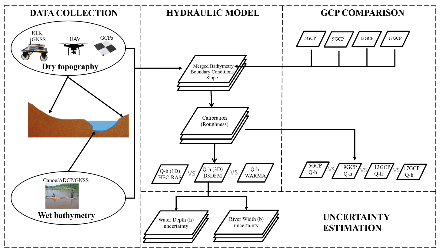
In brief, the experiment consists of the following steps: (i) select a suitable study site as far away as possible from impediments which may cause backwater effects and with a relatively straight river profile; (ii) use a combination of the UAV, real-time kinematic positioning (RTK) global navigation satellite system (GNSS), and acoustic Doppler current profiler (ADCP) to determine the wet and dry bathymetry and slope; (iii) merge the dry and wet bathymetries; (iv) subject the merged bathymetry to boundary conditions for a 3D-hydraulic-modelling environment; (v) determine the roughness coefficient; (vi) run the hydraulic model with different flow rates until a relationship between flow and stage (rating curve) can be determined; and (vii) compare the rating curve with traditional rating curves, then repeat this experiment using varying bathymetries, and compare the outputs to determine if there is a significant difference in the results. Figure 1 presents a schematic of the experiments conducted in this study.
2.1 Data collection methods
A detailed description of how the dry and wet river bathymetry can be collected using low-cost UAV and GNSS devices is introduced in Sect. 2 of Samboko et al. (2022a). The method involves merging of photogrammetry-based dry bathymetry with a volumized wet bathymetry through linear interpolation to produce one seamless bathymetric point cloud. The dry bathymetry is a DEM generated from geotagged images captured from a UAV, and the wet bathymetry is generated from a river transect measured using an ADCP with an RTK GNSS device mounted to it to establish precise locations. Alvarez et al. (2018) conducted a similar study describing how a DEM obtained by lidar or photogrammetry can be combined with the bathymetry (obtained by echo sounding). In short, the method consists of the following steps. An airborne instrument (e.g. UAV) is used to collect overlapping and geotagged images, which are in turn converted into dry bathymetry through photogrammetry. Ground control points measured using low-cost RTK GNSS equipment are used to rectify inaccuracies in the bathymetry. The wet bathymetry is measured using a combination of an RTK GNSS and an echo sounding instrument (e.g. fish-finder). The waterline is then measured using the RTK GNSS so as to correct any doming effect which may be caused by uncertainties in correcting radial lens distortions. Finally, the wet and dry bathymetries are merged through linear interpolation to form a seamless full bathymetry.
2.2 Study site
The study was conducted in southern Zambia along the Luangwa River, downstream of the Luangwa Bridge. The basin has a catchment area of approximately 160 000 km2. The Luangwa River originates in the Mafinga Hills in the north-eastern part of Zambia and is approximately 850 km in length, flowing in the south-western direction (The World Bank, 2010). The river drains into the Zambezi River, shaping a broad valley along its course, which is well known for its abundant wildlife and relatively pristine surroundings (WARMA, 2016). The study area is approximately 25 ha.
For purposes of comparison, the specific location of the study site is only a few kilometres from the Zambia Water Resources Management Authority (WARMA) permanent gauging station and a couple hundred metres from the site where a similar study based on a 1D Hydrologic Engineering Center – River Analysis System (HEC-RAS) model was conducted (Abas et al., 2019). These sites may be considered similar in their hydraulic conveyance properties, given that they are geographically close to each other, and their geomorphological characteristics are similar. A data set of discharge and stage measurements, taken by WARMA between 1948 and 2002, is available for rating curve comparison. We surveyed the flow and water level twice, at the end of the rainy season and at the end of the dry season, so as to capture both low- (only permanent channel) and intermediate-flow (also partly floodplain) conditions. These ADCP-based flow measurements were contemporary with the GCP and bathymetry measurements. Figure 2a shows the location of the study site within the Luangwa basin. Figure 2b shows the location of the study site in relation to the two other sites: the WARMA gauging station and the location where Abas et al. (2019) conducted a similar study based on a 1D model.
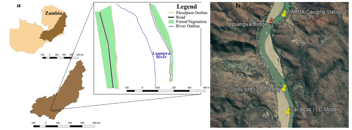
Figure 2(a) Study site along Luangwa River, (b) location of study site in relation to other comparison sites (© Google Maps 2022).
2.3 Hydraulic modelling
For hydraulic simulation, we used a software called D-Flow Flexible Mesh (D3DFM; Deltares, 2020). D3DFM solves the nonlinear shallow-water equations in 1D, 2D, or 3D or combinations thereof using a flexible-mesh domain. Within D3DFM two different layering methods are provided for 3D models, the sigma (σ) method and the Z method. The Z method is based on the Cartesian Z-coordinate system, resulting in straight horizontal coordinate lines. Layers in the σ model increase or decrease their thickness as the water depth in the model increases or decreases. The relative thickness distribution of the different layers however remains fixed (Deltares, 2020).
A hydraulic model consisting of a bed level, a grid structure, mathematical formulations describing the physical processes, and corresponding necessary assumptions and approximations requires boundary conditions to simulate the desired hydraulic processes. In the case of a river model these boundary conditions do often comprise an inflow and outflow of water implied by a discharge, velocity, or water level. In D3DFM models these boundary conditions can be imposed as a time series or as a harmonic signal. Besides the boundary conditions, there are initial conditions and physical parameter values to be assigned to the model, for example initial water levels, the water temperature, and a uniform friction coefficient. This friction coefficient influences the maximum velocity of the water at the river bed and therefore affects the discharge capacity and water level in the simulation (Saleh et al., 2013). The roughness can be described by different formulations like Chézy, Manning, or White–Colebrook, which all contain a certain roughness coefficient that needs to be specified. For the purpose of this study, the Manning coefficient is chosen as it is more applicable to open channels (Zidan, 2015).
2.4 Description of data requirements for D3DFM
Model set-up and evaluation needed the bathymetry, boundary conditions (discharge and water level), and roughness coefficient. The bathymetry of the terrain is established through merging and volumization of photogrammetric data with sonar measurements. In brief, the digital terrain model (dry bathymetry) is merged with river transects (wet bathymetry) and subsequently volumized into a complete seamless bathymetric point cloud through linear interpolation. More details on this method can be found in Samboko et al. (2022a).
The seamless bathymetry is then cut perpendicular to the flow direction on both sides in preparation for input into D3DFM. Figure 3 shows an example of a DEM which has been volumized and subsequently cut on both sides.
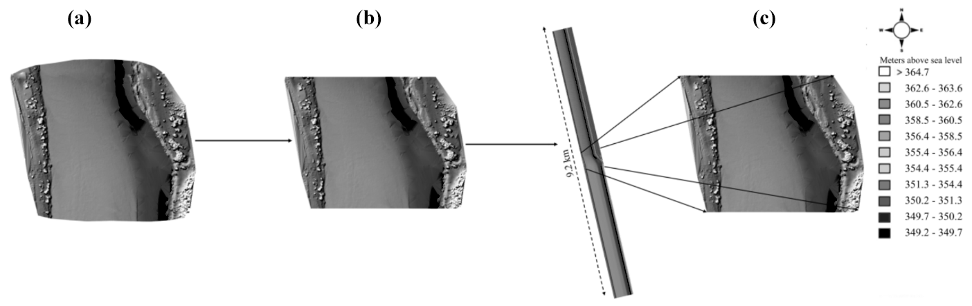
Figure 3(a) Study site volumized bathymetry, (b) bathymetry cut on both sides perpendicular to flow, (c) elongated elevation model imported into D3DFM.
In order to use the point cloud in a model, the area should be extended both downstream and upstream. The extensions are required to ensure that upstream water can numerically spread over the entire width realistically and to ensure that downstream backwater effects do not significantly alter water levels in the area of interest. In order to extend the point clouds using representative samples, a small selection of 1200 coordinates over the complete width on each side is taken. This small stretch is reproduced every 36 m in the direction of flow (or opposite for the extension to the north). This means the longitudinal and latitudinal values are shifted slightly, and the height is subtracted from or added to the corresponding slope. The point cloud is extended both upstream and downstream with 118 stretches, corresponding to 4248 m, which is significantly more than the adaptation length (2.1 km). The adaptation length is the distance required to counter the effects of backwater. After volumizing the model for the last time, the final result is a point cloud containing 4.76 × 10⁹ coordinates representing approximately 9.2 km of the Luangwa River.
2.5 D3DFM set-up, calibration, and evaluation
The model was set up with two Manning roughness configurations: one based on the main channel using the dry-season observation set (water level, flow, and velocimetry) and another where the degrees of freedom are extended to two roughness values (one main channel, one floodplain) using an observation taken during both the wet- and dry-season observations. This is to evaluate whether one visit is sufficient or whether multiple visits are recommended.
In order to determine the optimal roughness coefficient of the main channel in the dry season, we constrained the model through optimization of a combination of surface velocity and water level. The start value for Manning's friction coefficient was set at 0.018 s m, the median of the n value (Manning) for sandy, straight uniform channels which ranges from 0.012 to 0.026 s m (Arcement and Schneider, 1989). The upstream boundary condition which was measured in the field was kept constant at 191 m3 s−1. We imported the surface velocity distribution, where the velocities were extracted using a technique called large-scale particle image velocimetry (LSPIV) and also measured using a current meter. Similarly, the water level profile, which was measured using an ADCP, was imported into the model and compared to the simulated water levels. Note that the use of an ADCP could be replaced by the use of a more cost-efficient sonar, such as a fish-finder device, to keep the method entirely affordable. The comparison is based on the mean average deviation (MAD), as shown in Eq. (1).
where n is the number of measurements, xi is the term in question, and μ is the mean of all measured values. The score was based on 5 measurements for the current meter and 10 for LSPIV. The simulated water level was similarly assessed, with five observation points located in the centre of the wet bathymetry. A combination which yields the lowest values of MAD indicates an optimal roughness coefficient to proceed with.
The second model set-up incorporated the wet and dry roughness coefficients. On the main channel, we applied the roughness which had been calibrated in the dry season. On the floodplain, we applied a roughness coefficient of 0.040 s m, which was derived through a 1D HEC-RAS model in the wet season. A summary of the derivation is described in Appendix A.
After the model was constructed and calibrated, the next step was to accurately predict discharges other than 191 m3 s−1. Establishing a stage–discharge relationship requires rating points (a discharge with the corresponding stage) produced by the model. Hence, the model was run at least 20 times with changing boundary conditions. The upstream boundary condition was given by a discharge ranging from 5 to 3000 m3 s−1, and the downstream boundary condition was determined through repetitive iterations. For each discharge the downstream water level was determined by iteration until the backwater curve did not exceed 3 cm in total. This is done by selecting three arbitrary points downstream of the river, then plotting the backwater curve, which should ideally be parallel to the bed surface. Finally, both models were compared with a traditional rating curve constructed by WARMA. The 95 % confidence interval of the WARMA rating curve is used to generally judge the accuracy of the more physically constructed rating curve. Statistical model evaluation tools, Nash–Sutcliffe efficiency (Ens), and percentage bias (Pbias) are also used to determine significant differences among the simulated curves. The selected criteria are recommended for model evaluation because of their robust performance rating in simulating models (Moriasi et al., 1983). Pbias measures the tendency of the simulated data to either underestimate or overestimate the observed WARMA readings. Low magnitudes indicate optimal model simulation. Ens indicates how well the plot of observed vs. simulated data fits the 1:1 line. Ens and Pbias are computed as shown in Eqs. (2) and (3).
where O is the observed value, Omean is the mean of all observed values, P is the simulated value, and x is the total number of values.
2.6 Comparison of discharge estimations based on varying geometries
In order to evaluate the impact of the number of GCPs on the estimated discharge, 4 elevation models reconstructed based on 5, 9, 13, and 17 GCPs are fed into the D3DFM hydraulic model under similar boundary conditions. The preparation of the bathymetries is similar to that described in Sect. 3.2. We inter-compare the different rating curves individually to evaluate if there are any notable differences. Figure 4 shows the varying GCP configurations used in the generation of bathymetries.
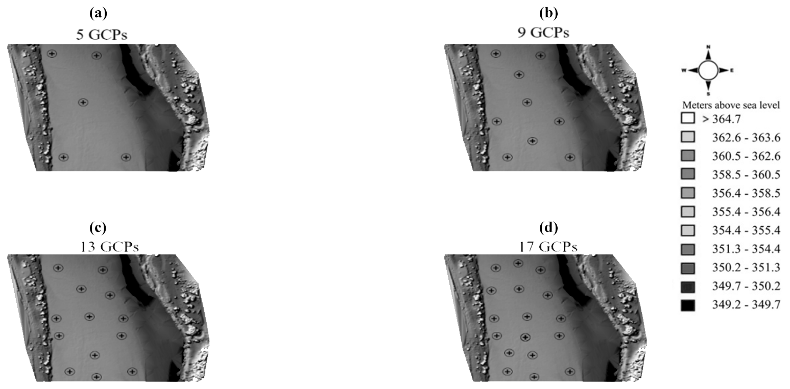
Figure 4GCP distribution along floodplain of the Luangwa River: (a) 5-GCP distribution, (b) 9-GCP distribution, (c) 13-GCP distribution, (d) 17-GCP distribution.
2.7 Evaluation of the propagation of continuous width and depth observations in uncertainty in discharge estimation
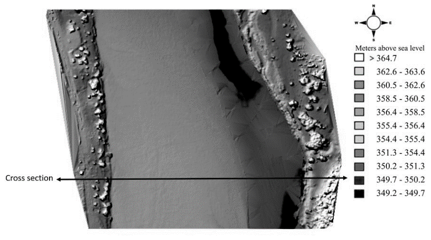
The two main proxies for flow that we assessed and which can potentially be used for continuous monitoring through satellite observations are water level and river width. In preparation for measuring river width, we placed a cross-section perpendicular to river flow where the cross-section must cut across the entire floodplain. Figure 5 shows the location and orientation of the cross-section.
Thereafter, the model is run 20 times with varying upstream boundary conditions between 5 and 3000 m3 s−1. For each simulated upstream discharge value, we measured and recorded the width in the simulation. After calculating the average river width we established a discharge vs. river width relationship (Q−b). With the assumption that our estimated widths could have uncertainties of ±5 m or in even more uncertain cases ±10 m, we estimated the river flow and its uncertainty through the established relationships between flow and depth and between flow and width, respectively. These uncertainty estimations were based on the resolution of satellite sensors we may rely on such as ICESat-2 for river depth and Sentinel-1 and Sentinel-2 for river width. This allowed us to assess at which point along the full stretch of the floodplain which proxy is more likely to produce accurate discharge estimations. This process was repeated with water depth as the proxy.
The impact of photogrammetry-based geometry on the estimated discharge was assessed through three steps: comparing the rating curve of the D3DFM model with traditional methods, comparing rating curves based on geometries constructed using different GCP numbers in D3DFM, and evaluating how the uncertainty in models based on proxies for flow (width and water level) propagate into discharge inaccuracies.
3.1 Comparing the rating curve of the D3DFM model with traditional methods
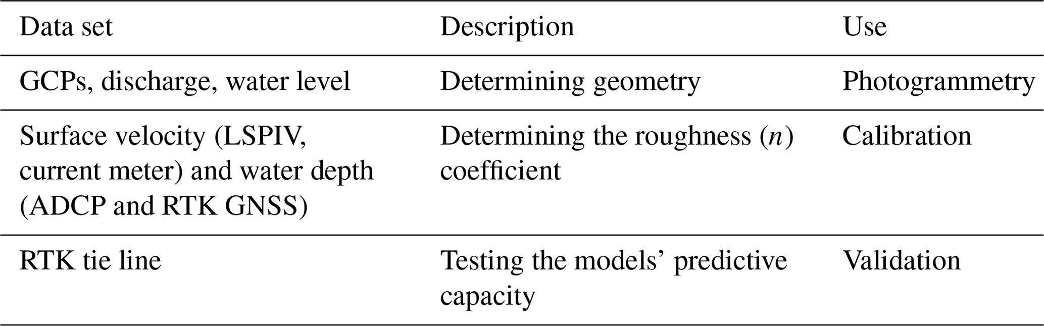
Before the comparison of D3DFM with other models, calibration and validation were performed. The surface flow velocity and the water depth were used to calibrate the model, whilst model validation was performed based on a visual assessment of the RTK tie line. The measured variables are summarized in Table 1. All the data were collected on the same day.
Table 1The experiments used for models' calibration and validation.
The model set-up required calibration of the roughness coefficient based on an optimal combination of the simulated water surface velocity and water level. The simulated velocities for the different roughness values were compared to the current meter and LSPIV measurements using the mean average deviation (MAD) and percentage bias. Table 2 provides the MAD of both the velocities and the water levels for each applied Manning coefficient (n). Lower values of MAD represent more optimal results.
Table 2Mean average deviation for roughness optimization.
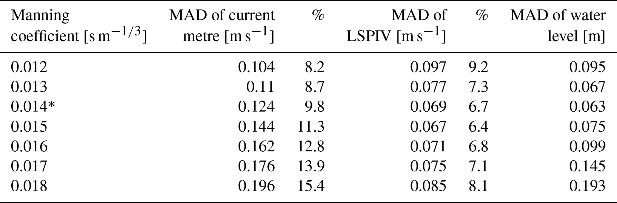
* The selected optimal roughness coefficient.
The first model simulation, which was set at 0.018 s m, shows a relatively high average deviation (CM: 15.4 %; LSPIV: 8.1 %) of the surface flow velocity and an overestimation of the water level by 0.193 m. This results in a substantial widening of the river due to the uniform “flat” floodplain. Both the velocity and the water level indicate a better performance when lower roughness values are applied since less resistance means faster-flowing water and a lower water level with equal discharge. After further reductions in roughness values, results indicate that velocity and water levels are optimal when the Manning coefficient is set at either 0.015 or 0.014 s m. These two values correspond to the lowest values of LSPIV (6.4 %) and water level (0.063 m), respectively. In order to determine which of the two to select we use the current meter MAD as the tie-breaker. Consequently, 0.014 s m (* in Table 2) is selected as the optimal roughness coefficient of the main channel.
The calibration of the roughness coefficient, which was based on the surface velocity, provides a unique opportunity to apply a non-contact, UAV-based method of model calibration. The LSPIV method was not only non-intrusive and safer to apply in the crocodile-infested river but also proved to be considerably more accurate than the current meter. For instance, at the chosen roughness coefficient of 0.014 s m, the mean average deviation percentage for the current meter is 9.8 %, but it is 6.7 % for the LSPIV method.
The model validation was performed based on a visual analysis of the alignment between the measured RTK tie line and the simulated water level. Figure 6 shows the RTK tie line, which was measured along the waterline, and the simulated flow at Q= 191 m3 s−1, n= 0.014 s m (main channel), and n= 0.040 s m (floodplain). In the absence of varying seasonal gauge readings, the alignment between the RTK tie line and the simulated waterline on the right bank of the river provides visual evidence of good model performance. In general, validation based on visual analysis is not as robust as a quantitative method. However, in certain data-scarce regions such as the Luangwa River, where the resources required to conduct multiple data collection campaigns are limited, it is useful to establish contingency methods which can provide indicators of discharge estimation accuracy. In spite of this, it is important to note that, for the purposes of assessing the quality and robustness of the physics-based hydraulic model, more discharge samples are required for quantitative model validation.
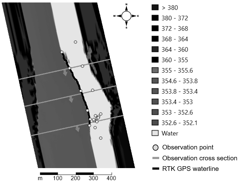
Figure 6Visual representation of the discharge model at a discharge of 191 m3 s−1 with n= 0.014 s m.
After the model was set up and evaluated, simulations ranging from 5 to 3000 m3 s−1 in increments of 100 m3 s−1 were performed. Figure 7 presents four rating curves: the first curve is based on a single-channel Manning coefficient (derived from a dry-season flow survey in the main channel), the second curve is based on a combination of two coefficients (main channel and floodplain), the third curve shows the rating curve based on a 1D HEC-RAS model, and the final curve is based on the conventional gauging method from WARMA. The discharge measurements are visualized in relation to a 95 % confidence interval of the WARMA rating curve. In addition to the confidence interval, we evaluated the significant differences among the curve-based Ens and Pbias in relation to the WARMA curve.
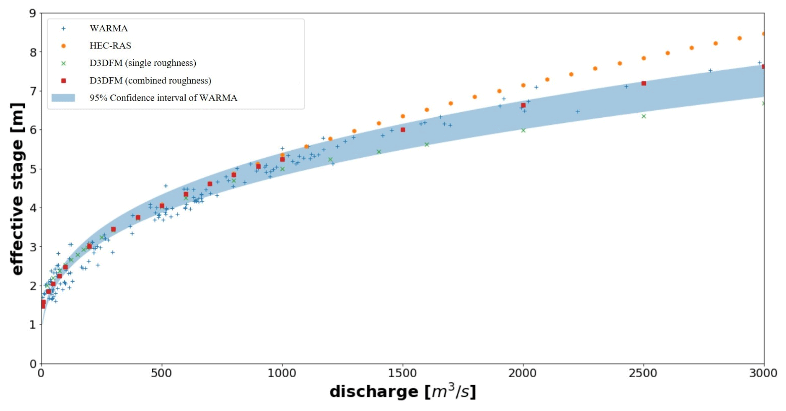
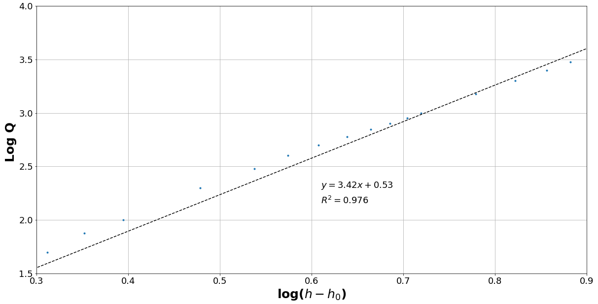
The D3DFM-based model, which combines two different roughness coefficients, more closely resembles the WARMA curve than the 1D HEC-RAS curve and the D3DFM, which applies only one roughness for the entire terrain. This is particularly the case for high-flow conditions. This result may be attributed to better optimization of the roughness coefficients (compared to 1D or 3D with only one Manning roughness), which acknowledges the fact that roughness in the main channel is different from roughness in the floodplain. It must be noted, however, that comparing with the relationships of WARMA and 1D HEC-RAS is only insightful to a certain extent as the experiment was not conducted at the exact same location as where the WARMA rating curve is maintained. Possible differences in the river geometry may cause our results to not be entirely equivalent to WARMA's rating curve. The final stage–discharge relationship is expressed by Fig. 8 and Eq. (4). This relationship should function as a basis on which adjustments can be made based on newly available stage–discharge data. Note that the river geometry will most likely change over time due to the sandy bed level, and therefore the constants are not stable over time.
3.2 Comparison of discharge based on varying GCP numbers
To assess the impact of the number of ground control points on the bathymetric chart and therewith on the modelled discharge, charts created with different GCP numbers were used to run the same hydraulic model with similar boundary conditions. Figure 9 presents the rating curves of all four distributions.
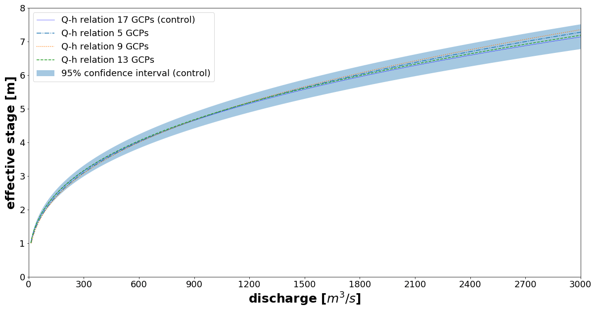
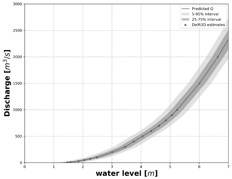
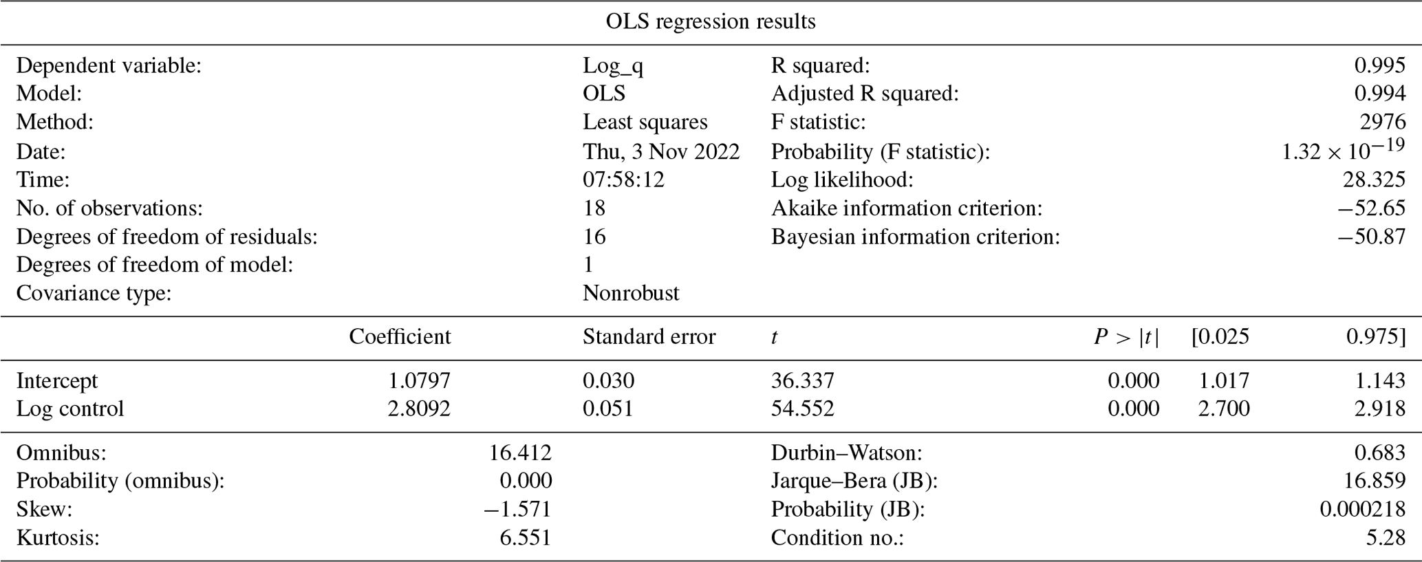
Assuming the bathymetry based on 17 GCPs as the control, we plotted a 95 % confidence interval on its rating curve. The confidence interval was plotted based on ordinary least squares (OLS) regression results. These results are presented in Appendix B. Using 17 GCPs as the standard of comparison, the Pbias and Ens results indicate very similar curves derived among bathymetries based on 5, 9, and 13 GCPs: Pbias of 3 %, 0.7 %, and 0.6 % and Ens of 0.982, 0.998, and 0.999, respectively. All four curves fell within the 95 % confidence interval of the control curve (17 GCPs). It must be noted that the bathymetry up until 191 m3 s−1 is determined by the ADCP and RTK measurements, and therefore the number of GCPs does not influence the curve up until this point. In this study, a minimum of five GCPs spread over 25 ha is sufficient for accurate discharge estimation. We draw a conclusion that for the purposes of physics-based river rating, a ratio of 5 ha per GCP is sufficient to accurately estimate discharge. However, in all instances, including terrains less than 1 ha, the minimum number of GCPs required is three to allow for triangulation (Oniga et al., 2020). Finally, it is important to note that the distribution of the GCPs is likely to influence the final chart drastically as the most uncertain areas will be at the borders of the bathymetry (mostly due to the bowling effect). Therefore an optimal GCP distribution will be representative of not only the full spectrum of elevations but also the priority placement of GCPs on the edges of the terrain being mapped.
3.3 The impact of uncertainty in proxies for flow on discharge estimation
Finally, we investigated the impact of proxy uncertainties (river width and water level) on discharge estimation. By proxies we mean variables that can be more easily observed operationally. We imposed uncertainty based on the resolution of satellite sensors we may rely on such as ICESat-2, as investigated by Coppo Frias et al. (2023) for river depth, and Sentinel-1 and Sentinel-2 for river width (Filippucci et al., 2022). Figure 10 presents the relationship between discharge and river width. The graph also highlights two different potential error intervals, ±5 m (90 %) and ±10 m (95 %), so as to visualize the amount of uncertainty which corresponds to specific sections of the terrain.
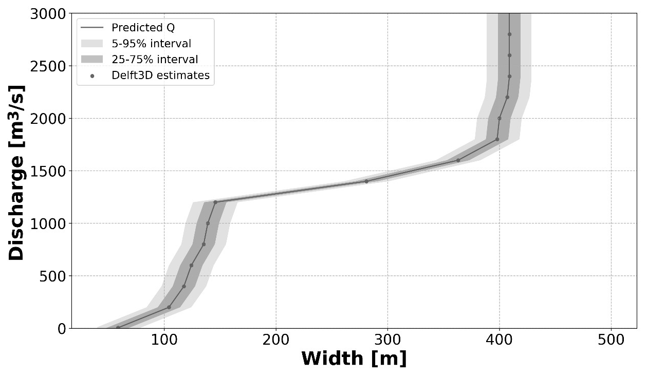
If river widths were used, this would result in high levels of flow uncertainty below 150 m. These higher levels of uncertainty are a result of low sensitivity of width to changes in flow below 150 m. The low sensitivity in this low-flow stage can be attributed to the steep bank; i.e. as flow increases, the depth rises quickly, but there are minimal changes in width. During medium-level flows, between 150 and 370 m, results indicate lower levels of width uncertainty, i.e. high river width sensitivity. The high sensitivity in this medium-flow stage may be attributed to the gently sloping floodplain; i.e. as flow increases, the width rises significantly faster than the water level. Finally, higher levels of width uncertainty are noted during high flows (above 370 m). This region experiences low sensitivity of width to changes in flow. The causal factor is inundation of the entire floodplain, which has not been included in the hydraulic schematization.
Similar to width, water level uncertainties also result in varying discharge estimates. Figure 11 presents the relationship between discharge and water level as simulated by D3DFM. The graph also highlights two different potential error intervals, ±10 cm (90 %) and ±20 cm (95 %). These error intervals assist us in visualization of the amount of uncertainty in flow that can be expected from using water levels as a proxy. For lower flows (< 1000 m3 s−1), results indicate lower levels of water level uncertainty, i.e. high water level sensitivity. The justification for the high sensitivity in this low-flow stage can be attributed to the steep bank; i.e. as flow increases, the depth rises quickly, but there are minimal changes in width. During medium-level flows, between 1000 and 1500 m3 s−1, results indicate higher levels of water uncertainty, i.e. low water level sensitivity. The low sensitivity in this medium-flow stage may be attributed to the gently sloping floodplain; i.e. as flow changes, the water level does not change significantly. Finally, during high flows the floodplain is inundated with water; thus, the expectation in this regime is high water level sensitivity, i.e. low water level uncertainty. Contrary to our expectation, this segment experiences high water level uncertainty. This may be because the magnitude is larger or because of lateral flow of water below thick forest on the left bank and disturbances from unnatural infrastructural development (e.g. the road) on the right bank maintain high levels of uncertainty.
As shown in Figs. 10 and 11, the proxies for flow (water level and river width) are antagonistic in nature. This implies that when one of the proxies exhibits high uncertainty, the other is more likely to present low levels of uncertainty.
We note that different proxies for flow, namely water level and river width, perform optimally at different segments. At low flows the shape of the wet river channel (steep slope) is more likely to induce high sensitivity of water level and low sensitivity of river width to changes in discharge. At higher flow levels the shape of the wet river channel (gentle slope) is more likely to induce low sensitivity of water level and high sensitivity of river width to changes in flow. At even higher flows, ideally, the floodplain is inundated and becomes insensitive to river width. In the absence of more accurate discharge estimation methods, the water level is once again the more reliable proxy. Above the natural levee, the assumptions of the schematization of the D3DFM model no longer hold, and therefore any flows above that level should not be considered reliable.
3.4 Discussion
This study offers the unique opportunity to compare a 1D model and a 3D model for the purpose of river discharge estimation. This comparison is made with the understanding that the 1D HEC-RAS model data (collected April 2019) were collected approximately one hydrological cycle (1 year) before the D3DFM model data (collected November 2020). Therefore, we were able to establish the roughness of two different flow regimes (high and medium flow). The comparison of two or more rating curves based on potentially varying bathymetries and floodplain geometries will not yield precisely identical results. However, the close proximity of the study sites and the hydrogeological similarities of the two locations mean that our ability to extract meaningful comparison is not compromised.
Results indicate that the 1D model is similar to the 3D model in its capacity to generate accurate rating curves for the purpose of river monitoring. In addition to being freely available (open-source), the 1D model requires significantly less computing power than the 3D model, which may be a limitation for water authorities with limited financial capabilities. However, we note two significant benefits of the 3D model over the 1D model. Firstly, the 3D model takes into account the heterogeneity of the river geometry and roughness at much higher spatial resolution. In contrast, the 1D model relies more on point-based measurements, which would suggest that the 3D model is capable of estimating more accurate flow discharge when applied correctly. Secondly, the 3D model introduces a unique validation method which is not available in the 1D model. We refer here to the ability to extract the surface velocity within the 3D model and compare it to surface velocities derived from direct methods such as the current meter or LSPIV. It is not possible to extract surface velocities from a 1D model.
Apart from comparing the 3D model with the 1D model, this study derived some validation by comparing the 3D model with traditionally derived rating curves. The fact that the more physics-based method was within a 95 % confidence interval of the WARMA (traditional curve) provides evidence that flow can be accurately estimated through non-contact means and constant improvement in technologies. However, in order to verify the robustness of the UAV-based system one would need to repeat the experiment with more than one rating curve method. In our opinion, it is reasonable to assume we can produce results similar to WARMA if the iterations are processed expertly.
The study reaffirms and provides insight into the potential of applying a combination of UAVs and other technologies for river discharge estimation. The methods described in the study are well within reach of water authorities with limited resources and are particularly useful for small- to medium-sized rivers in sub-Saharan Africa. The D3DFM discharge model resembles actual river depth, width, and location when using a combination of two Manning coefficients (0.014 and 0.040 s m) and a discharge value of 191 m3 s−1.
Based on the PBIAS and Ens values, there is no significant difference in estimated discharge for bathymetries reconstructed based on 5, 9, 13, and 17 GCPs. Five GCPs is sufficient to simulate a curve which falls within the 95 % confidence interval of a WARMA curve (control). Therefore, five GCPs is adequate for physically based river rating under the condition that the GCPs are accurately measured using an RTK GNSS and are optimally distributed to represent the full spectrum of terrain elevations.
The slope, which is an important input to the model, must be measured as accurately as possible for the longest possible distance along the waterline. Ideally, measuring the waterline height at 200 m intervals for a 5 km stretch is sufficient to avoid the impact of wave distortions. The impact of backwater distortions is of particular concern for high water levels as opposed to low water levels, and therefore a longer measuring distance is required in high-water-level instances. However, the magnitude of slope has a bearing on the length that is required to reduce the impact of backwater distortions; i.e. in the Luangwa River's case, a long distance would be needed, but for streams with a large bottom slope, a much shorter distance is sufficient. Furthermore the stretch chosen for observation must be long enough to cancel out the effects of sand banks (uneven silt deposition), which may have an impact on the slope accuracy. However, identifying and measuring such long stretches is problematic due to difficult terrains and inaccuracies caused by the need to move the base station. The most feasible compromise is to use one base station location and then measure continuously for as far as possible to both sides, use correction via satellites, or use a spirit level. In that way the relative accuracy stays the same and will be very good.
We determined that the proxies for flow (water level and river width) perform well at different stages of discharge. For instance, at low discharge values and steep banks, the water level is more sensitive to changes in flow and thus more accurate. For higher discharge values and gentle floodplain slopes where the floodplain fills up, the river width is more sensitive to flow changes and thus more appropriate to use. As a result of the two proxies performing in opposition to one another, a combination of both methods in different flow regimes gives a more accurate flow monitoring assessment. Alternatively, determining the river geometry first and then deciding which proxy is most appropriate to apply would be most helpful. In instances where the slope is gentle, the width would be more appropriate since a slight change in discharge has a larger impact on river width. The opposite is true for steeply sloping river beds. In instances where the slope is steep, the water level would be more appropriate since slight changes in discharge would have a larger impact on water level.
We reiterate that the accurate measurement of a tie line is critical not only to correct the doming effect but also to provide an extra validation check for the hydraulic model. In this study we demonstrate that this is feasible and affordable using a simple combination of an RTK GNSS and a mobile cart. The tie line must be measured simultaneously with the river discharge so that it can be compared against the simulated waterline as derived by the hydraulic model. Finally, we recommend that the approach is applied in the dry season so as to minimize the amount of water flowing in the river for more efficient photogrammetry processing. However, it is important to occasionally measure flows and corresponding water levels at different times of the year so as to validate the efficiency of the model simulation and differentiate roughness in the main channel and floodplain.
In this Appendix, we describe a preliminary study which was conducted in order to determine the optimal roughness coefficient during high flows. The preliminary research was conducted in close proximity to the study currently in question. Both study locations have similar geophysical and hydraulic properties and thus are comparable. The research methodology was divided in four stages. The first stage was data collection of discharge, bathymetry and aerial data. A DJI Phantom 4 uncrewed aerial vehicle (UAV) with a 12 MP camera was used to collect. The second stage was processing of images and transects collected using the UAV and ADCP, respectively. The images were merged together and used to reconstruct the dry topography through photogrammetry. The third stage involved hydraulic modelling using the HEC-RAS model. The 1D steady-state hydraulic model was built and calibrated based on the ADCP measurements. In the final stage, the more physically based rating curve from the hydraulic model was compared with a traditional rating curve from the Zambian Water Resources Management Authority (WARMA).
The model output was evaluated by the root mean square error (RMSE). The lowest value for the RMSE is obtained for a Manning roughness coefficient of n= 0.040 s m. According to the literature this seems to be a reasonable value. We proceed to utilize this roughness value in the current study as a representation of the optimal roughness during high flows.
All data (including UAV images) used in this paper can be found at https://doi.org/10.4121/14865225 (Samboko, 2021). The coding scripts can used can be found at https://doi.org/10.4121/21557148 (Samboko et al., 2022b).
HTS: conceptualization, data curation, formal analysis, investigation, and writing of the original draft. HW: conceptualization, reviewing, editing, and supervision. SS: data collection, curation, and investigation. HM: supervision, reviewing, and editing. KB: reviewing and editing. HHGS: acquisition of funds, supervision, reviewing, and editing.
The contact author has declared that none of the authors has any competing interests.
Publisher’s note: Copernicus Publications remains neutral with regard to jurisdictional claims in published maps and institutional affiliations.
This work is part of the research programme ZAMSECUR with grant number W 07.303.102, which is financed by the Netherlands Organisation for Scientific Research (NWO). This research received and continues to receive support from the University of Zambia and the Zambian Water Resources Management Authority.
This research has been supported by the Nederlandse Organisatie voor Wetenschappelijk Onderzoek, Stichting voor de Technische Wetenschappen (grant no. W 07.303.102).
This paper was edited by Flavia Tauro and reviewed by two anonymous referees.
Abas, I., Luxemburg, W., Banda, K., and Hubert, S.: A robust approach to physically-based rating curve development in remote rivers through UAV imagery, Geophys. Res. Abstr., 21, 2019–5765, 2019.
Alvarez, L. V., Moreno, H. A., Segales, A. R., Pham, T. G., Pillar-Little, E. A., and Chilson, P. B.: Merging Unmanned Aerial Systems (UAS) Imagery and Echo Soundings with an Adaptive Sampling Technique for Bathymetric Surveys, Remote Sens., 10, 1362, https://doi.org/10.3390/RS10091362, 2018.
Arcement, G. J. and Schneider, V. R.: Guide for selecting Manning's roughness coefficients for natural channels and flood plains, Water Supply Pap., 38, 2339, https://doi.org/10.3133/WSP2339, 1989.
Awasthi, B., Karki, S., Regmi, P., Dhami, D. S., Thapa, S., and Panday, U. S.: Analyzing the Effect of Distribution Pattern and Number of GCPs on Overall Accuracy of UAV Photogrammetric Results, Lect. Notes Civ. Eng., 51, 339–354, https://doi.org/10.1007/978-3-030-37393-1_29, 2019.
Coppo Frias, M., Liu, S., Mo, X., Nielsen, K., Ranndal, H., Jiang, L., Ma, J., and Bauer-Gottwein, P.: River hydraulic modeling with ICESat-2 land and water surface elevation, Hydrol. Earth Syst. Sci., 27, 1011–1032, https://doi.org/10.5194/hess-27-1011-2023, 2023.
Coveney, S. and Roberts, K.: Lightweight UAV digital elevation models and orthoimagery for environmental applications: data accuracy evaluation and potential for river flood risk modelling, Int. J. Remote Sens., 38, 3159–3180, https://doi.org/10.1080/01431161.2017.1292074, 2017.
Deltares: D-Flow Flexible Mesh User Manual, https://oss.deltares.nl/web/delft3dfm/manuals (last access: 13 November 2022), 2020.
Dey, S., Saksena, S., and Merwade, V.: Assessing the effect of different bathymetric models on hydraulic simulation of rivers in data sparse regions, J. Hydrol., 575, 838–851, https://doi.org/10.1016/J.JHYDROL.2019.05.085, 2019.
Ferrer-González, E., Agüera-Vega, F., Carvajal-Ramírez, F., and Martínez-Carricondo, P.: UAV photogrammetry accuracy assessment for corridor mapping based on the number and distribution of ground control points, Remote Sens., 12, 2447, https://doi.org/10.3390/RS12152447, 2020.
Filippucci, P., Brocca, L., Bonafoni, S., Saltalippi, C., Wagner, W., and Tarpanelli, A.: Sentinel-2 high-resolution data for river discharge monitoring, Remote Sens. Environ., 281, 113255, https://doi.org/10.1016/J.RSE.2022.113255, 2022.
Kim, Y.: Uncertainty analysis for non-intrusive measurement of river discharge using image velocimetry, https://www.gettextbooks.com/isbn/9780542833311/ (last access: 6 January 2019), 2006.
Liu, X., Zhang, Z., Peterson, J., and Chandra, S.: Large Area DEM Generation Using Airborne LiDAR Data and Quality Control, Spatial Accuracy Assessment in Natural Resources and Environmental Sciences, World Academic Union, 77–85, 2008.
Martínez-Carricondo, P., Agüera-Vega, F., Carvajal-Ramírez, F., Mesas-Carrascosa, F. J., García-Ferrer, A., and Pérez-Porras, F. J.: Assessment of UAV-photogrammetric mapping accuracy based on variation of ground control points, Int. J. Appl. Earth Obs., 72, 1–10, https://doi.org/10.1016/J.JAG.2018.05.015, 2018.
Moriasi, D. N., Arnold, J. G., Van Liew, M. W., Bingner, R. L., Harmel, R. D., and Veith, T. L.: Model evaluation guidelines for systematic quantification of accuracy in watershed simulations, T. ASABE, 50, 885–900, https://doi.org/10.13031/2013.23153, 1983.
Oniga, V. E., Breaban, A. I., Pfeifer, N., and Chirila, C.: Determining the suitable number of ground control points for UAS images georeferencing by varying number and spatial distribution, Remote Sens., 12, 876, https://doi.org/10.3390/RS12050876, 2020.
Rafik, H. and Ibrekk, H. O.: Environmental and Water Resources Management Environment Strategy Papers No. 2 Rafik Hirji Hans Olav Ibrekk, https://api.semanticscholar.org/CorpusID:127266855 (last access: 14 April 2023), 2001.
Saleh, F., Ducharne, A., Flipo, N., Oudin, L., and Ledoux, E.: Impact of river bed morphology on discharge and water levels simulated by a 1D Saint-Venant hydraulic model at regional scale, J. Hydrol., 476, 169–177, https://doi.org/10.1016/J.JHYDROL.2012.10.027, 2013.
Samboko, H. T., Abasa, I., Luxemburg, W. M. J., Savenije, H. H. G., Makurira, H., Banda, K., and Winsemius, H. C.: Evaluation and improvement of Remote sensing-based methods for River flow Management, Phys. Chem. Earth, 117, 102839, https://doi.org/10.1016/j.pce.2020.102839, 2019.
Samboko, H. T.: Photogrammetry Images from DJI P4, point clouds scripts and supporting data, 4TU.ResearchData [data set], https://doi.org/10.4121/14865225, 2021.
Samboko, H. T., Schurer, S., Savenije, H. H. G., Makurira, H., Banda, K., and Winsemius, H.: Evaluating low-cost topographic surveys for computations of conveyance, Geosci. Instrum. Method. Data Syst., 11, 1–23, https://doi.org/10.5194/gi-11-1-2022, 2022a.
Samboko, H. T., Savenije, H. H. G., and Winsemius, H.: Python Scripts used in the study: Towards Affordable 3D Physics-Based River Flow Rating: Application Over Luangwa River Basin, 4TU.ResearchData [code], https://doi.org/10.4121/21557148, 2022b.
Skondras, A., Karachaliou, E., Tavantzis, I., Tokas, N., Valari, E., Skalidi, I., Bouvet, G. A., and Stylianidis, E.: UAV Mapping and 3D Modeling as a Tool for Promotion and Management of the Urban Space, Drones, 6, 115, https://doi.org/10.3390/DRONES6050115, 2022.
Smith, M. W., Carrivick, J. L., and Quincey, D. J.: Structure from motion photogrammetry in physical geography, Prog. Phys. Geog., 40, 247–275, https://doi.org/10.1177/0309133315615805, 2015.
The World Bank: The Zambezi River Basin, Technical report, Washington D.C., https://documents1.worldbank.org/curated/en/938311468202138918/pdf/584040V30WP0Wh110State0of0the0Basin.pdf (last access: 14 August 2022), 2010.
WARMA: Luangwa Catchment, http://www.warma.org.zm/index.php/%0Acatchments/luangwa-catchment (last access: 4 September 2019), 2016.
Woodget, A. S., Austrums, R., Maddock, I. P., and Habit, E.: Drones and digital photogrammetry: from classifications to continuums for monitoring river habitat and hydromorphology, Wiley Interdiscip. Rev.-Water, 4, e1222, https://doi.org/10.1002/WAT2.1222, 2017.
Zidan, A.: Review of friction formulae in open channel flow, Int. Water Technol., 5, https://www.researchgate.net/publication/320456925_REVIEW_OF_FRICTION_FORMULAE_IN_OPEN_CHANNEL_FLOW (last access: 15 August 2023), 2015.
- Abstract
- Introduction
- Material and methods
- Results and discussion
- Conclusion and recommendations
- Appendix A: One-dimensional HEC-RAS model
- Appendix B: OLS regression results
- Code and data availability
- Author contributions
- Competing interests
- Disclaimer
- Acknowledgements
- Financial support
- Review statement
- References