Collaborative development of the Lidar Processing Pipeline (LPP) for retrievals of atmospheric aerosols and clouds

Atmospheric lidars can simultaneously measure clouds and aerosols with high temporal and spatial resolution and hence help understand cloud–aerosol interactions, which are the source of major uncertainties in future climate projections. However, atmospheric lidars are typically custom-built, with significant differences between them. In this sense, lidar networks play a crucial role as they coordinate the efforts of different groups, provide guidelines for quality-assured routine measurements and opportunities for side-by-side instrument comparisons, and enforce algorithm validation, all aiming to homogenize the physical retrievals from heterogeneous instruments in a network. Here we provide a high-level overview of the Lidar Processing Pipeline (LPP), an ongoing, collaborative, and open-source coordinated effort in Latin America. The LPP is a collection of tools with the ultimate goal of handling all the steps of a typical analysis of lidar measurements. The modular and configurable framework is generic enough to be applicable to any lidar instrument. The first publicly released version of the LPP produces data files at levels 0 (raw and metadata), 1 (averaging and layer mask), and 2 (aerosol optical properties). We assess the performance of the LPP through quantitative and qualitative analyses of simulated and measured elastic lidar signals. For noiseless synthetic 532 nm elastic signals with a constant lidar ratio (LR), the root mean square error (RMSE) in aerosol extinction within the boundary layer is about 0.1 %. In contrast, retrievals of aerosol backscatter from noisy elastic signals with a variable LR have an RMSE of 11 %, mostly due to assuming a constant LR in the inversion. The application of the LPP for measurements in São Paulo, further constrained by co-located AERONET data, retrieved a lidar ratio of 69.9 ± 5.2 sr at 532 nm, in agreement with reported values for urban aerosols. Over the Amazon, analysis of a 6 km thick multi-layer cirrus found a cloud optical depth of about 0.46, also in agreement with previous studies. From this exercise, we identify the need for new features and discuss a roadmap to guide future development, accommodating the needs of our community.

1 Introduction

Aerosols, clouds, and their interactions are the source of the largest uncertainties in current climate change estimates (IPCC, 2013, 2023). More frequent and higher-quality measurements of aerosol, clouds, and the physical processes governing their link with climate are needed to reduce these uncertainties (Mather, 2021; National Academies of Sciences, Engineering, and Medicine, 2018), and lidars are a powerful instrument to accomplish this task (Reagan et al., 1989). This instrument can provide information on the optical and microphysical properties of aerosol particles and hydrometeors; the concentration of trace gases; and more recently the 3D structure of the vegetation and urban canopies, allowing ecologists to estimate biomass content accurately and engineers to develop self-driving cars and drones (Wang and Menenti, 2021).

Atmospheric lidars in particular measure the atmosphere's constituents from the troposphere to the mesosphere. However, they are developed by individual groups for particular applications; hence their hardware characteristics differ in essential aspects, such as receiving optics, emitted and detected wavelengths, polarization capability, and signal-to-noise ratio, to name a few. Even in the realm of single-wavelength elastic lidars, typical differences between custom-built lidar systems are large enough to require a careful, dedicated analysis of their return signals (Wandinger et al., 2016). In this sense, lidar networks play a crucial role as they coordinate the efforts of different groups, providing the guidelines for quality-assured routine measurements on a regional scale (Antuña-Marrero et al., 2017). Moreover, the coordinated effort is of utmost importance to homogenize the physical retrievals from the highly non-uniform instruments in lidar networks, which typically involves comparing the retrievals based on the algorithms of different groups (Pappalardo et al., 2004) and the instruments themselves (Wandinger et al., 2016). This homogenization is only possible by developing a unified processing pipeline that accounts for the hardware heterogeneity in the pool of instruments, as has recently been accomplished in the context of the European Aerosol Research Lidar Network (EARLINET) (D'Amico et al., 2015) and the Asian Dust and Aerosol Lidar Observation Network (AdNet) (Sugimoto and Uno, 2009). In contrast, homogeneous networks have the advantage of uniform calibration and data processing procedures, like those performed by the NASA Micro Pulse Lidar NETwork (MPLNET) (Welton et al., 2001), the Italian Automated LIdar-CEilometer network (ALICEnet) (Dionisi et al., 2018), or the Raman and Polarization Lidar Network (Polly^NET) (Baars et al., 2016).

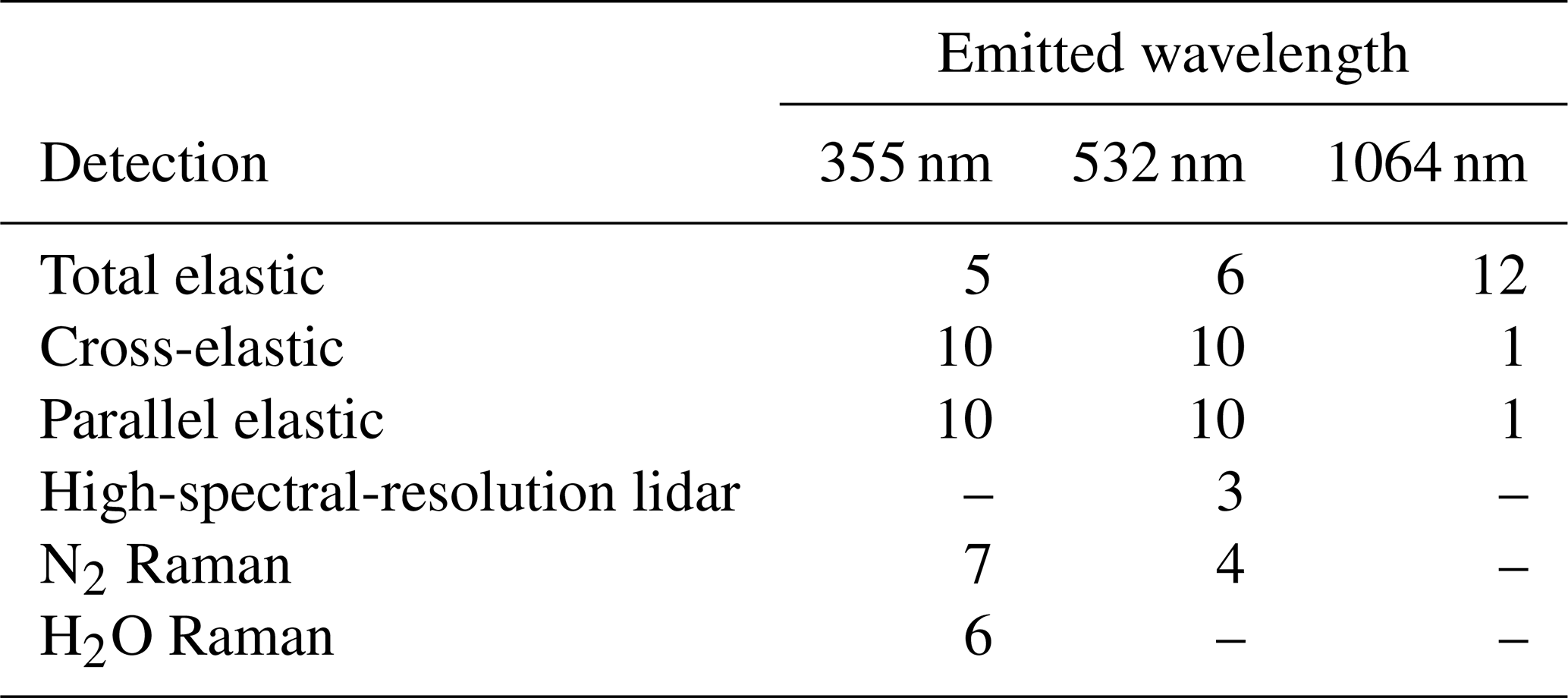
The Latin America Lidar Network (LALINET) (Landulfo et al., 2016) is a Latin American coordinated heterogeneous lidar network to obtain extensive and intensive aerosol optical properties profiled in the atmosphere. This federated lidar network aims to establish a consistent and statistically sound database to enhance the understanding of aerosol distribution over Latin America and its direct and indirect influence on climate. There are currently 19 stations in 6 countries, most of which are equipped with tropospheric aerosol lidars measuring one or more elastic return signals; only a few systems can measure inelastic return signals, typically for N₂ and H₂O Raman scattering. Table 1 shows the wide distribution of emitted wavelengths and detection modes. Other significant differences are found in the laser repetition rate (ranging from 10 to 30 Hz), beam expander factor (1 to 5×), mirror diameter (20 to 50 cm), telescope focal length (1 to 4 m), and width of the interference filters (0.25 to 1 nm). Finally, only a few stations have co-located or nearby measurements of the aerosol optical depth and the thermodynamic profile. More details about the network can be found in Landulfo et al. (2020).

Table 1 Number of stations in LALINET for each combination of emitted wavelength and detection mode (status as of 2023). More details about the network can be found in Landulfo et al. (2020).

In recent years, the LALINET network has worked towards establishing routine quality-assurance tests and intercomparing the retrieval algorithms used by the different groups (Guerrero-Rascado et al., 2016; Barbosa et al., 2014a). Here, our first goal is to present a high-level overview of the Lidar Processing Pipeline (LPP), an ongoing and unfunded coordinated effort to homogenize the retrievals from different lidar instruments in Latin America. Our second goal is to introduce the tools developed to handle all the steps of a typical lidar analysis. We want to emphasize the modular framework that is generic enough to be applicable to any lidar instrument or network and, at the same time, also highlight the open-source character of the LPP development (see “Code availability”). Our third goal is to show how the LPP performs through quantitative and qualitative analyses of synthetic and measured lidar signals. We discuss case studies based on synthetic and measured signals and analyze aerosol backscatter retrievals for elastic lidar signals and layer masking (clouds or aerosol), which are the focus of this first public release of the LPP.

The rest of this paper is organized as follows. Section 2 presents the overall concept of the LPP, the algorithms, and the structure of the different levels of output files. Sample results from the application of the LPP to actual lidar data from two LALINET stations are presented in Sect. 3. Current limitations, future perspectives, and conclusions are given in Sect. 4.

2 Processing pipeline

The Lidar Processing Pipeline is being developed in a partnership between the lidar groups of the Latin American Lidar Network. The LPP reads a series of raw data files in the standard Licel format (Licel GmbH, 2023) and produces a NetCDF file containing its data level products 0, 1, and 2. The processing pipeline has three main modules responsible for data processing at each level, all written in C/C$++$, which can run on Linux, Mac, or Windows. These modules are independent, and the whole pipeline can be automated with a script, or each module can be run directly in a terminal.

The modules are driven by a single configuration file, and the input data for each module are the output file produced in the previous stage, as can be seen schematically in Fig. 1. Moreover, the output file of a given level (e.g., 2) contains all the content of the previous level (e.g., 1) in addition to the new information generated in that level of data processing. In other words, all the information used to process the data to a given level is available in the corresponding file, thus allowing its reprocessing if needed. Figure 2 shows the content of a level 2 data file. The following sections explain the concept of each data level.

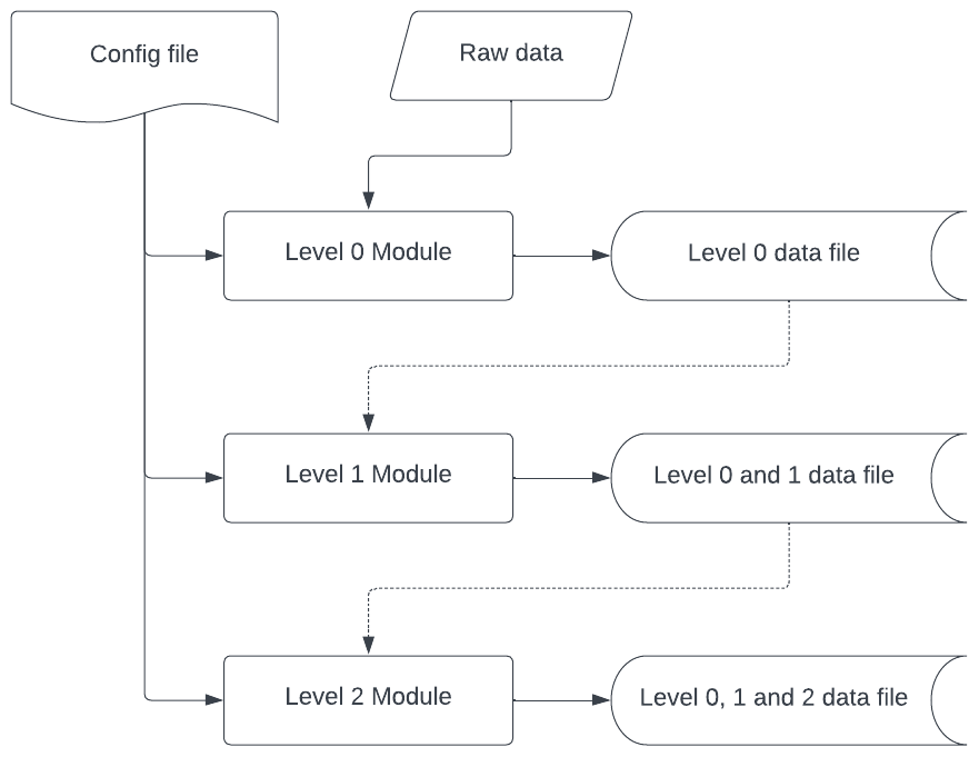
Figure 1 Flow diagram showing the structure of LPP version 1.1.2. Each module receives as input the data file produced as output in the previous module. A single configuration file is used for all the modules.

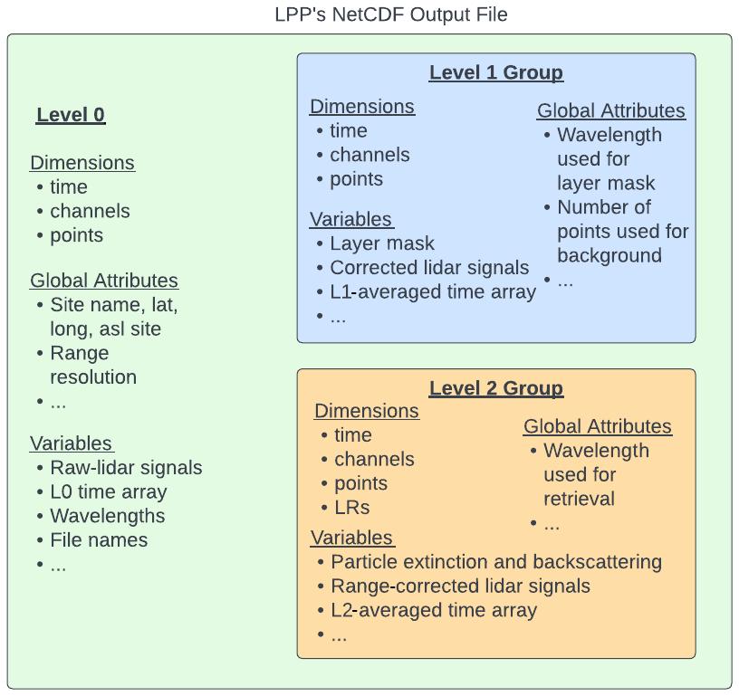
Figure 2 Schematic structure of the output files. Product data levels 1 and 2 are stored in subgroups named LX Data, while data level 0 data are stored in the file root tree. Dimensions and variables are explained in detail in the LPP's documentation on the GitHub repository (see “Open Science Development” section).

2.1 Data level 0 (L0)

The main goal of the level 0 data processing is to convert all the data files containing the lidar profiles into the standard LPP format used for all data levels. At this stage, there is no smoothing, averaging, or processing of any kind. The level 0 module simply dumps all information from a series of raw lidar files into a single output file. This includes all the information from the header of the raw files that describe the measurements, the instrument, and the site, such as filename; site name; start and stop time of the measurement; altitude, latitude, and longitude of the site; zenith and azimuth angles of the lidar signals (in the case of scanning lidars); accumulated laser pulses; laser repetition rate; and the number of channels acquired. These parameters are described in the Licel transient-recorder user manual (Licel GmbH, 2023). For each channel, the following information is saved: channel ID, polarization state, type (elastic/Raman), number of height bins, photomultiplier voltage, and wavelength. For analog channels, the number of bits and range of the analog-to-digital converter (ADC) are recorded, while for photon-counting channels, the discriminator level is recorded (Licel GmbH, 2023). For each channel, the raw ADC counts are saved as two-dimensional arrays indexed in height and time. Therefore, level 0 data consist of ADC counts for both analog and photon-counting channels; i.e., the raw values are not converted to millivolts (analog) or megahertz (photon counting). Figure 2 gives an overview of the file structure.

2.2 Data level 1 (L1)

The main goal of level 1 data processing is to apply the necessary corrections to the lidar profiles and compute a layer mask, which usually requires accumulating multiple profiles to increase the signal-to-noise ratio. The level 1 module receives a single level 0 data file as input, which contains all the raw signals and associated metadata, and produces a single level 1 file as output (see Fig. 2).

In the current version, the following corrections are implemented based on Guerrero-Rascado et al. (2016) and Freudenthaler et al. (2018). The first is the trigger delay correction. This accounts for the possible delay between the emission of the laser pulse and the start of the data acquisition, resulting in a vertical displacement of the measured signals, which affects both analog and photon-counting channels. The trigger delay can be measured by the so-called zero-bin (for the analog channels) and bin-shift (for the photon-counting channels) tests. Each channel has a different time delay, given in terms of an integer number of range bins and set in the configuration file. The correction consists of discarding these first few bins so that all channels start in sync with the laser pulse. The total length is also cropped so that all channels have the same length.

Second is the dark-current correction, which accounts for the signal distortions due to the acquisition system. Typical examples are transient peaks from firing the laser flashlamp and time-dependent electronic noise in analog channels, which are measured in the absence of light entering the telescope. If a dark-current test has been performed, a file with this information can be provided, and the dark current for each channel will be subtracted from the corresponding measurements.

Third is the background correction, which accounts for sky radiation entering the telescope, which is unrelated to the lidar signal. This is due to scattered sunlight or moonlight, which produce a constant noise in the return signal but would also include electronic noise if the dark-current correction were not applied. The background noise can be found by averaging the signal in a high altitude range, defined in the configuration file, where the lidar signal is completely extinguished. Alternatively, it can be found by performing a so-called Rayleigh fit. In this case, it corresponds to the constant term in a linear least squares fit between the lidar signal and the molecular signal, as in Grigorov and Kolarov (2013) and Barbosa et al. (2014b).

Besides the corrections and time averaging, L1 data also include the temperature and pressure profiles provided by the user. The input thermodynamic profile can be obtained from any source, such as radiosondes, weather forecasts, or reanalysis. Alternatively, the LPP includes and could use thermodynamic profiles from the US standard atmosphere (National Geophysical Data Center, 1992).

Finally, the L1 data processing creates a layer mask to indicate the presence of aerosol and cloud layers. The method is based on the ideas proposed by Vaughan et al. (2004), where the return signal is compared to the expected molecular signal. The threshold for detecting a layer is calculated dynamically, based on signal noise. Hence it can be applied to the wide range of instruments in the LALINET network. The time-averaged resolution for this product can be different than the one used in data level 2. The layer mask shows if there is a layer present (cloud or plume) by reporting a value of 1 and 0 otherwise. An example of the cloud layer mask is given in the “Results and discussion” section.

2.3 Data level 2 (L2)

The main goal of level 2 data processing is obtaining the profiles of aerosol optical properties, namely backscatter (m⁻¹ sr⁻¹) and extinction coefficients (m⁻¹). Additional time and vertical averaging might be applied to L2 data; hence it might be different from that of L1 data. The level 2 module receives a single level 1 data file as input, which includes the thermodynamic profile and corrected lidar signals, and produces a single level 2 file as output.

In this first release of the LPP, the optical properties are obtained from the analog elastic channels using the Fernald method (Fernald, 1984). The value of the lidar ratio (LR), assumed to be constant, is set by the user in the configuration file. When multiple LR values are given, the inversion is performed for each value, producing a set of optical properties. An example of the multi-LR retrieval is given in the “Results and discussion” section. The reference height, z₀, is not determined automatically and must be set by the user in the configuration file. The reference signal, P(z₀), which we assume contains no aerosol contribution, can be calculated either by averaging the signal or by taking the value of the molecular fit at the reference height. In both cases, this is evaluated in an altitude range defined by the user. The aerosol optical depth (AOD) is calculated assuming the extinction to be constant below a specific range (defined in the configuration file), where the incomplete overlap precludes its calculation.

3 Validation

Analyses of synthetic and measured lidar signals are carried out to demonstrate the usage of the LPP and to provide quantitative and qualitative validation of our initial results. These analyses are based on elastic signals, which are the focus of this first public release of the LPP. For a quantitative evaluation, we obtain the backscatter and extinction coefficients in the presence of aerosols or clouds and compare our results with the input used for the simulations, AERONET retrievals of aerosol optical depth (Holben et al., 1998), or LR values reported in the literature. For a qualitative evaluation, we obtain the cloud layer mask and compare it with the range-corrected lidar signal (RCLS) by visual inspection. The subsections below give the details of the four cases considered for validation.

3.1 Synthetic elastic lidar signals

We use two sets of synthetic lidar signals. The first is a simple case of an ideal lidar signal without noise and constant LR with altitude, provided by colleagues from TROPOS, in Germany (Holger Baars, personal communication, 2014). The aerosol profile has a constant extinction coefficient of 1100, 800, and 460 Mm⁻¹ at 355, 532, and 1064 nm, respectively, from the surface to the top of the boundary layer at 1.5 km. Above that height, it decreases every 250 m, reaching almost zero at 2.5 km. The residual aerosol in the free troposphere has an extinction of 0.014, 0.01, and 0.0058 Mm⁻¹ at 355, 532, and 1064 nm, respectively. The LR is fixed at 28, 39, and 77 sr at these wavelengths.

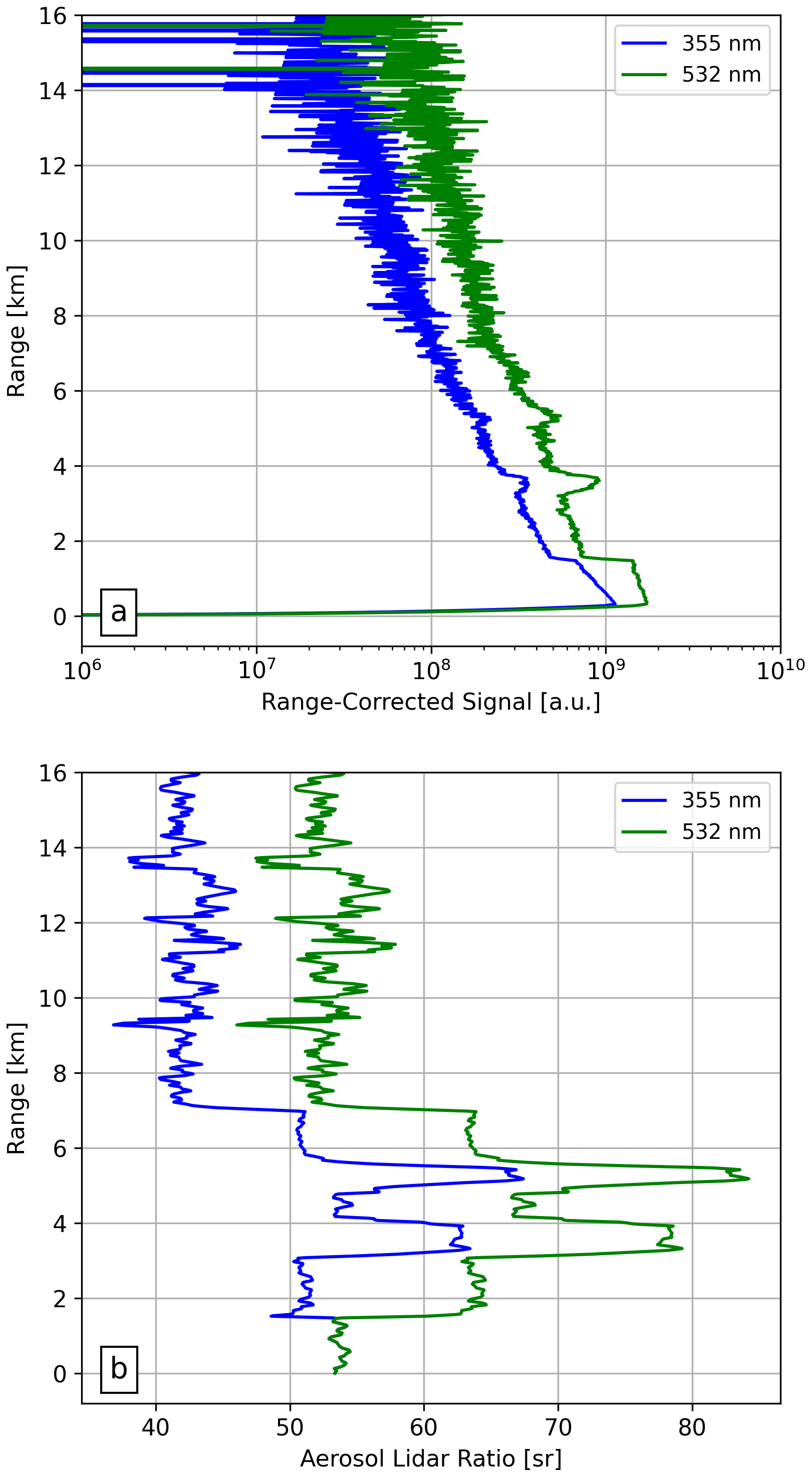
The second set of simulations corresponds to a more realistic case where the signals have noise, and the LR varies with altitude. These are the synthetic signals described and analyzed by Pappalardo et al. (2004) in the context of EARLINET's intercomparison of aerosol Raman lidar algorithms. This same dataset, which includes elastic signals at 355, 532, and 1064 nm and inelastic Raman signals at 387 and 607 nm, was used later to test the accuracy of the single calculus chain (SCC) optical products (Mattis et al., 2016). Three layers are clearly identified in this simulated atmosphere, denoted as a planetary boundary layer (PBL, from 0 to 1500 m), the free troposphere (FT, from 1500 to 3000 m), and a lofted layer (LL, 3000 to 7000 m). The dataset has 30 profiles with a 2 min resolution, corresponding to 2400 laser shots per profile (20 Hz laser), and a total acquisition time of 30 min. Spatial resolution is 15 m. For our analysis, we consider the average 355 and 532 nm elastic signals only.

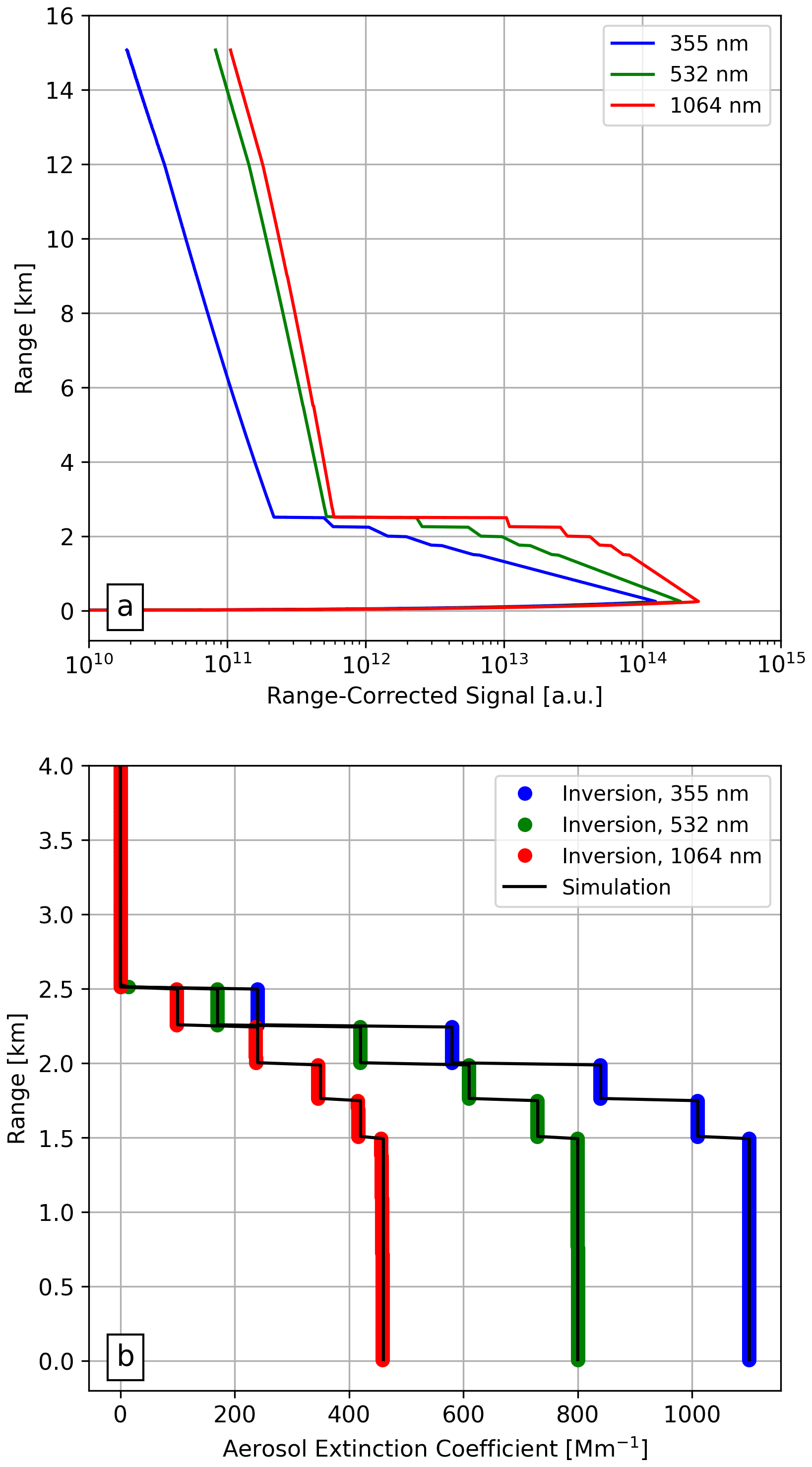
Figure 3 (a) Synthetic range-corrected signals (arbitrary units) and (b) aerosol extinction coefficients (Mm⁻¹) retrieved with the LPP (bullets) and used as input for the simulation (black lines) are shown for 355, 532, and 1064 nm.

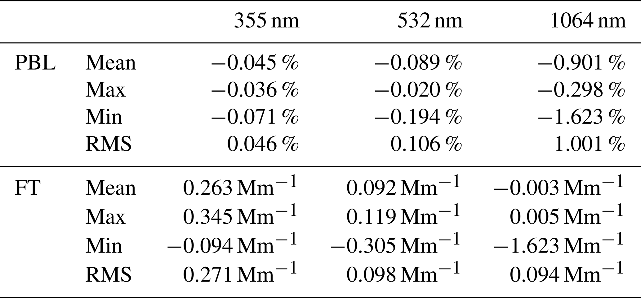
Table 2 Mean, maximum, minimum, and root mean square deviations in the retrievals of the extinction coefficient (Mm⁻¹) at 355, 532, and 1064 nm. Values in the PBL (250 to 2500 m) are expressed as relative deviations (%), while values in the free troposphere (FT, above 2500 m) are given in inverse megameters.

Both sets of synthetic signals include the effect of incomplete overlap in the near field to mimic a real measurement. We ignore this range for the inversions with the LPP and analyze the profile only where the overlap is complete. Both simulations also include information on the thermodynamic profile, which we use for calculating the molecular signal.

3.2 Case studies

To further validate the LPP and demonstrate its application to real data, we analyze elastic return signals from the LALINET lidar stations in São Paulo and Manaus, both in Brazil. With over 21.5 million inhabitants, São Paulo is the largest metropolitan region in the Americas. One of the primary sources of air pollution there is vehicular emissions, and the city has struggled with high levels of traffic congestion for many years (Andrade et al., 2017). During the winter (June to September), this can be exacerbated by temperature inversions, which inhibit mixing between the planetary boundary layer and the free atmosphere above. This well-stratified atmosphere shows high aerosol particle number concentrations within the boundary layer and a mostly clean atmosphere above it. While the air quality can vary depending on a number of factors, including weather patterns and traffic, we evaluate measurements from the São Paulo lidar station on a typical winter day, 14 September 2020.

The lidar deployed at São Paulo (23^∘56^′S, 46^∘74^′W; 740 m a.s.l.) is a multiwavelength Raman lidar operated by the Environmental Laser Applications research group at the Lasers and Applications Center (CLA), Nuclear and Energy Research Institute (IPEN) (Landulfo et al., 2020). It is a monostatic coaxial system, vertically pointed to the zenith and using a commercial Nd:YAG laser by Quantel, Brilliant B model, at a repetition rate of 10 Hz. The output energy per pulse is 850 mJ for 1064 nm, 400 mJ for 532 nm, and 230 mJ for 355 nm. A 300 mm diameter telescope with a 1.5 m focal distance and 1 mrad field of view (FOV) is used as a collection system, reaching a full overlap at 300 m above ground level. The detection box collects six different wavelengths: 355 and 532 nm elastic signals with the corresponding shifted Raman signals from nitrogen, 387 and 530 nm, respectively, as well as the water vapor line at 408 nm and the elastic signal from 1064 nm. The electronic acquisition system is a Licel transient recorder model TR-20-160.

The second set of measurements is taken from the Manaus lidar station in the Amazon rainforest. The site is located about 20 km upwind from the city; hence it is not affected by the significant urban emissions (Nascimento et al., 2022). Therefore, the atmosphere is mostly pristine throughout the year, with the exception being the dry season (June to October), when long-range transport of biomass burning affects the whole basin (Artaxo et al., 2013), and aerosols can be found up to 5 to 6 km (Baars et al., 2012). There is a marked diurnal cycle of convection, even during the dry season, with a peak in the late afternoon (Tanaka et al., 2014). Cirrus produced from the outflow of deep convective clouds are omnipresent, with a frequency of occurrence much higher than other tropical regions (Gouveia et al., 2017b). Here, we analyze a case of multi-layered cirrus clouds measured during the dry season, on 15 August 2011.

The lidar deployed in Manaus (2.89^∘ S, 59.97^∘ W; 100 m a.s.l.) is a UV Raman lidar operated by the University of São Paulo (Barbosa et al., 2014b). It is a biaxial system pointed 5^∘ from the zenith and uses a commercial Quantel CFR-400 Nd:YAG laser at 355 nm with 95 mJ per pulse and a 10 Hz repetition rate. The receiving telescope has a 400 mm primary mirror, a focal length of 4000 mm, and a field of view of about 1 mrad, reaching a complete overlap at 1.5 km. The detection box measures three wavelengths: elastic 355 nm and the corresponding Raman signals from nitrogen at 387 nm and water vapor at 408 nm. Data acquisition uses a Licel transient recorder model TR-20-160 with a raw resolution of 7.5 m.

Figure 4 (a) Synthetic range-corrected signals (arbitrary units) and (b) aerosol lidar ratio (sr) used as input for the simulation are shown for 355 and 532 nm. The retrievals shown in Fig. 5 assumed constant lidar ratios of 51 and 62 sr, respectively.

4 Results and discussion

To validate the LPP's first results, we performed the inversion of two sets of synthetic lidar signals and two sets of measurements from lidar systems in LALINET: a station in São Paulo, the largest metropolitan area in South America, and a station in Manaus, in the central Amazon rainforest. The simulations and the case studies exploit and highlight the features of the LPP's first release.

4.1 Noiseless synthetic signals with constant LR

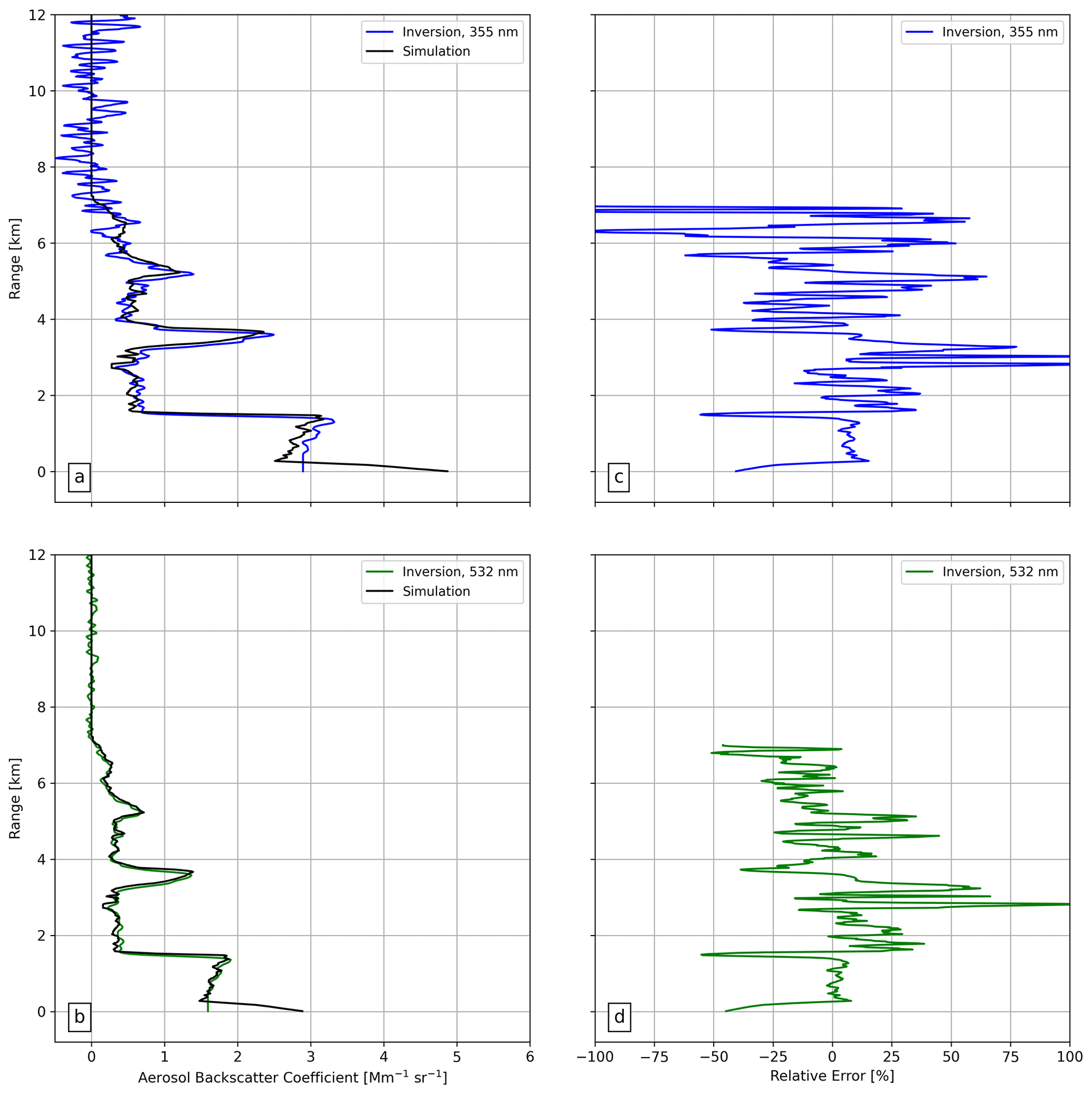
Figure 5 The left panels show a comparison of the aerosol backscatter coefficient (Mm⁻¹ sr⁻¹) retrieved at (a) 355 nm and (b) 532 nm with those used as input for the simulation (black lines). The right panels show the respective relative errors (%) where there are aerosols.

The RCLSs from the first simulation are shown in Fig. 3a for the three wavelengths. RCLSs are suitable for plotting since they remove the inverse-squared range dependence in the raw lidar signal, making it better for visualizations. The lack of noise in these signals makes finding the right reference value easier, reducing systematic errors related to this input parameter. Moreover, no vertical smoothing or time averaging was necessary. The inversions were performed using a reference altitude of 10 km and the true lidar ratio. Figure 3b shows the retrieved aerosol extinction coefficient and the input used for the simulation, showing excellent visual agreement.

To quantify the small differences that might exist between the retrieval and the simulated profile, we computed the deviation as a function of altitude, and Table 2 reports the mean, maximum, minimum, and root mean square deviations in the boundary layer and in the free troposphere. There is a small negative bias within the boundary layer, where the relative deviations are always negative. The mean values are −0.045 %, −0.089 %, and −0.901 % for 355, 532, and 1064 nm, respectively. Overall, the errors are greater for 1064 nm. In the free troposphere, where the aerosol loading is almost zero, there is a small positive bias. The mean deviations are 0.26, 0.092, and 0.003 Mm⁻¹ for 355, 532, and 1064 nm, respectively.

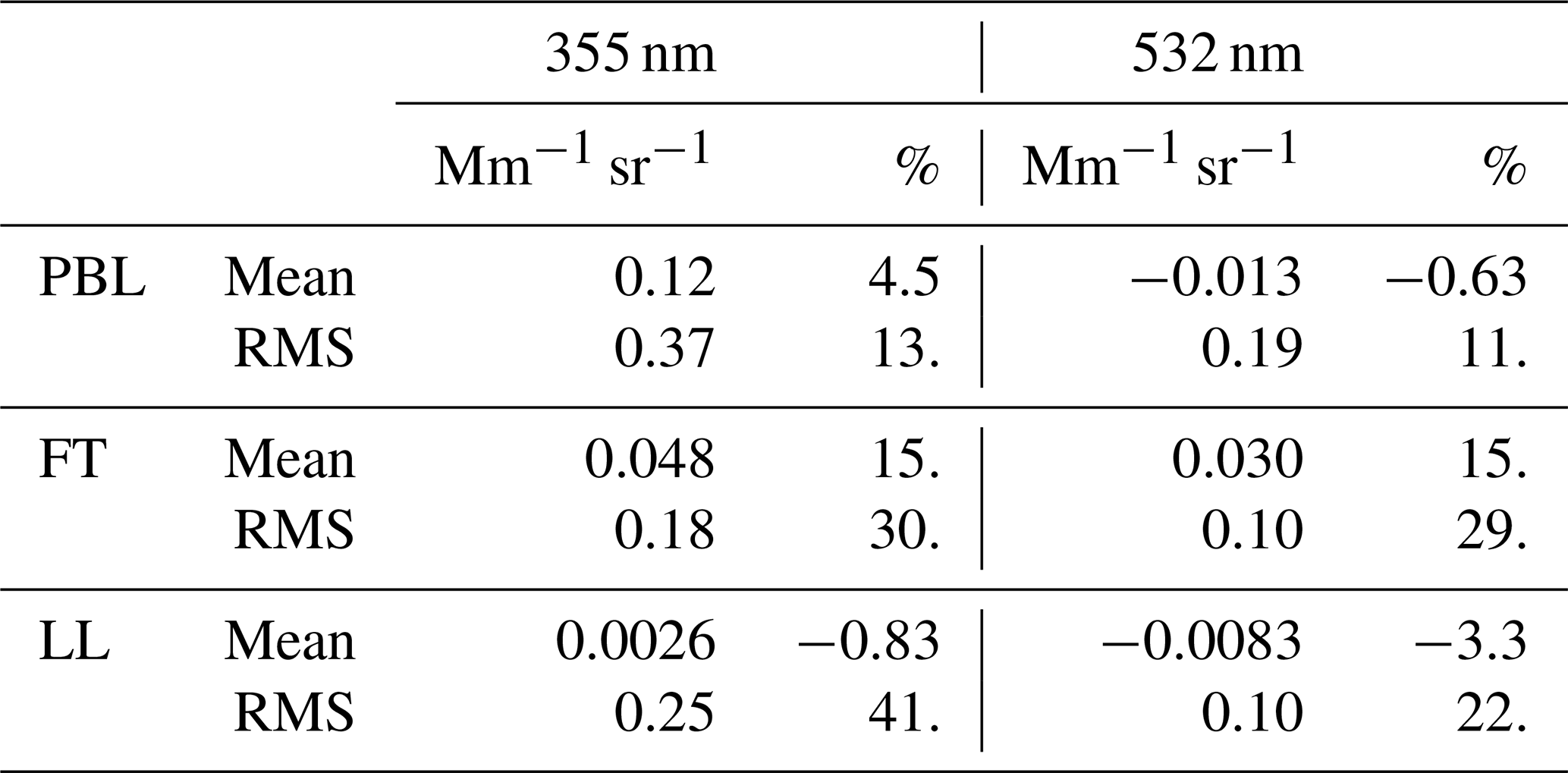
Table 3 Mean, root mean square, and relative errors in the retrievals of the backscatter coefficient at 355 and 532 nm in the PBL (280 to 1500 m), free troposphere (FT, 1500 to 3000 m), and lofted layer (LL, 3000 to 7000 m). Values are reported in absolute (Mm⁻¹ sr⁻¹) and relative (%) terms.

These errors are smaller than those reported by Böckmann et al. (2004) in a similar validation exercise in the context of EARLINET. Their case 2 considered an aerosol layer extending up to 4 km altitude, with constant LR, and the synthetic signals did not include noise. For stage 3 of their intercomparison, all 18 groups used the same LR and reference value at the calibration height. The mean relative error within the aerosol layer was 1.87 %, 1.48 %, and 1.38 % for 355, 532, and 1064 nm, respectively. While their synthetic profile was not the same as that used here, this initial comparison gives confidence that the LPP works well and can reproduce the simulations without biases if all input parameters are known.

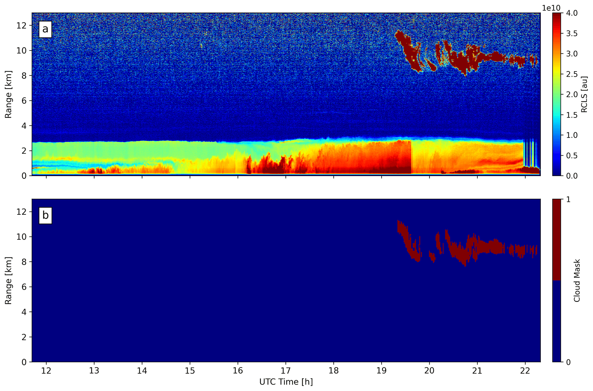
Figure 6 (a) RCLSs and (b) cloud layer mask for the São Paulo lidar station on 14 September 2020.

4.2 Realistic synthetic signals with variable LR

The average signals from the set of realistic simulations, which includes signal noise and a variable LR, are shown in Fig. 4. As this release of the LPP considers a constant LR for the inversion of the elastic signals, we computed the mean of the LR profile below 7 km, where the simulated aerosols are. The values were 51 sr for 355 nm and 62 sr for 532 nm, which were the same as the constant values used by Mattis et al. (2016) to test the accuracy of SCC optical products. The reference height was set to 9 km for both wavelengths, with the molecular range between 7.5 and 10.5 km. Signals were vertically smoothed by applying a five-point moving average, corresponding to an effective resolution of 75 m.

Figure 5a and b show the retrieved aerosol backscatter coefficients at both wavelengths. There is very good agreement overall, despite our assumption of a constant LR. According to EARLINET requirements, relative errors in the optical retrievals at 355 and 532 nm should be below 20 % or 0.5 Mm⁻¹ sr⁻¹ (Mattis et al., 2016). The relatively higher values obtained with the LPP occur for relatively lower values of the backscatter coefficient, which indicates that this is related to the signal noise and hence could be minimized with stronger vertical smoothing. There are also large errors at the altitudes where the input LR makes a sudden change, which can only be resolved by implementing the range-dependent LR solution for the elastic signal (Klett, 1985) or by implementing the Raman solution (Ansmann et al., 1992).

The mean errors for the three aerosol layers and the two wavelengths are shown in Table 3. The layer-mean relative errors are smaller than EARLINET's limits, with the largest values (about 15 %) found in the free troposphere, where the true LR profiles deviate the most from our assumed constant values. Root mean square relative errors are larger, reaching up to 41 % in the LL for 355 nm; however, these depend on the applied vertical smoothing as discussed above. Overall, the errors reported in Table 3 are similar to those found for EARLINET's SCC (Mattis et al., 2016). This shows that the LPP's retrievals do not have significant biases and can appropriately reproduce the realistic synthetic profiles.

4.3 Case study: São Paulo

The day chosen for this case study was 14 September 2020, a Monday near the end of the dry season. It was cloudless for most of the day, with some high clouds starting at 19:00 UTC (local time is UTC−3). We analyzed the elastic return signals at 532 nm, with no time averaging (raw level 1 resolution was 1 min). Figure 6 shows the color maps of the RCLS and its cloud layer mask. Aerosols are trapped in the boundary layer below 2.5 km. The diurnally forced convective boundary layer starts near the surface around 12:00 UTC (09:00 LT) and grows until it is fully developed around 18:00 UTC (15:00 LT). It takes over the nocturnal residual layer from the previous day, which can be seen in green colors during the first hours of the day.

Here we focus on the cloudless profiles between 12:00 and 18:00 UTC, when AERONET's level 2.0 AOD data were available for comparison. The inversion of the elastic signals was performed by the LPP level 2 module for 10 min time-averaged profiles, assuming constant LR values ranging from 30 to 100 sr, with steps of 5 sr (15 values). Hence, LPP level 2 data files have the time series of extinction, backscatter profiles, and the AODs for each tentative LR. AOD is calculated by integrating each of the extinction profiles, assuming them to be constant below 300 m to avoid the incomplete overlap region for this particular lidar station. Figure 7 shows the aerosol backscatter obtained from the multi-LR inversion at 12:53 UTC. Figure 8a shows the time series of AOD values for the same LR values that can be compared with the AERONET retrievals shown in black.

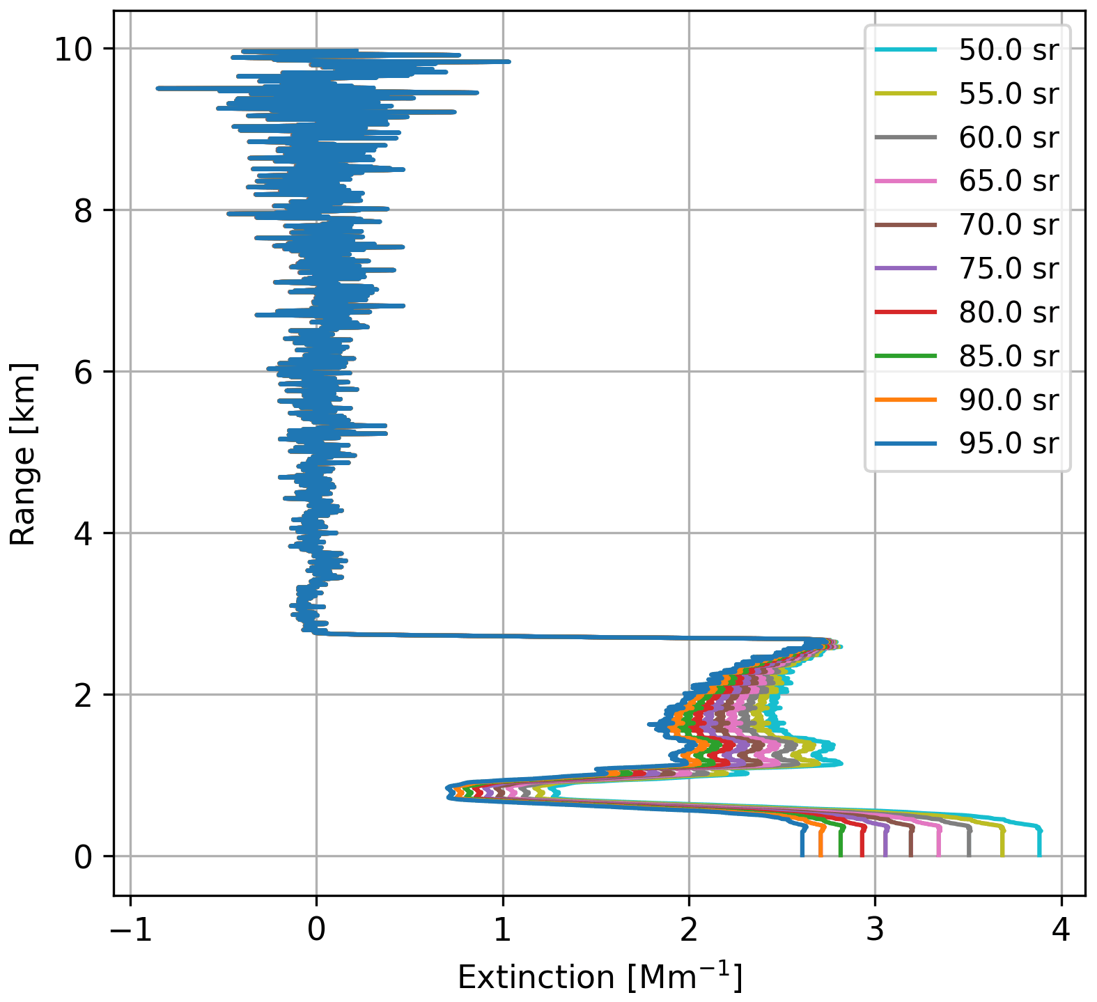
Figure 7 Aerosol backscattering coefficient obtained for the São Paulo lidar station on 14 September 2020 from 12:53 to 13:03 UTC using a set of predefined lidar ratios. The extinction coefficient is assumed constant below 300 m.

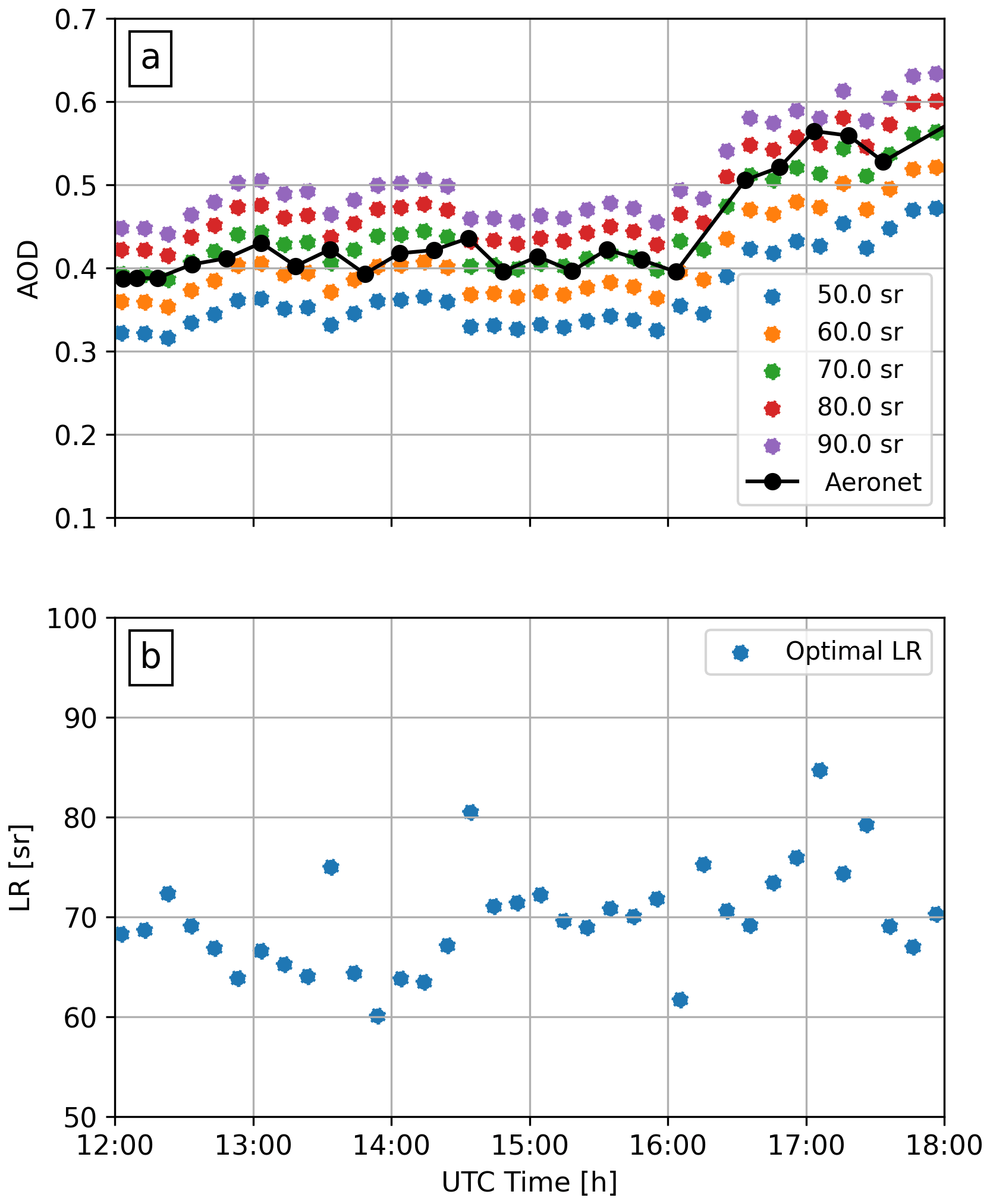
Figure 8 (a) AOD at 532 nm measured by AERONET (black) and obtained by the multi-LR lidar product using a set of predefined lidar ratios (colors) for the São Paulo lidar station on 14 September 2020 from 12:00 to 18:00 UTC. (b) Optimal LR values derived from each inversion.

Using 15 LRs allows us to search for which LR value produces the closest AOD value measured by AERONET. Here, this is done a posteriori, during the analysis of the multi-LR inversion. The time series of the optimal LR values is shown in Fig. 6b. Most of the values are between 60 and 80 sr, with a mean of 69.9 sr and a standard deviation of 5.2 sr, well within the range of values expected for urban aerosols (Ansmann and Müller, 2005). This initial evaluation shows that the LPP is performing well for real lidar data and demonstrates how the multi-LR retrieval can be used to constrain the optical properties obtained from elastic-only measurements.

4.4 Case study: Manaus

For this second case study, we focus on measurements of cirrus clouds performed on 15 August 2011. Previous studies in the Amazon region showed that their frequency of occurrence is higher than in other tropical regions and that they can have an important radiative effect (Gouveia et al., 2017a). Figure 9 shows a color map of the RCLSs and the corresponding cloud layer mask from the level 1 data, where a thin multi-layered cirrus between 10 and 16 km is clearly seen. The acquisition time of each lidar profile was 1 min, and no time average was used for this layer mask retrieval, which clearly captured the whole cirrus cloud.

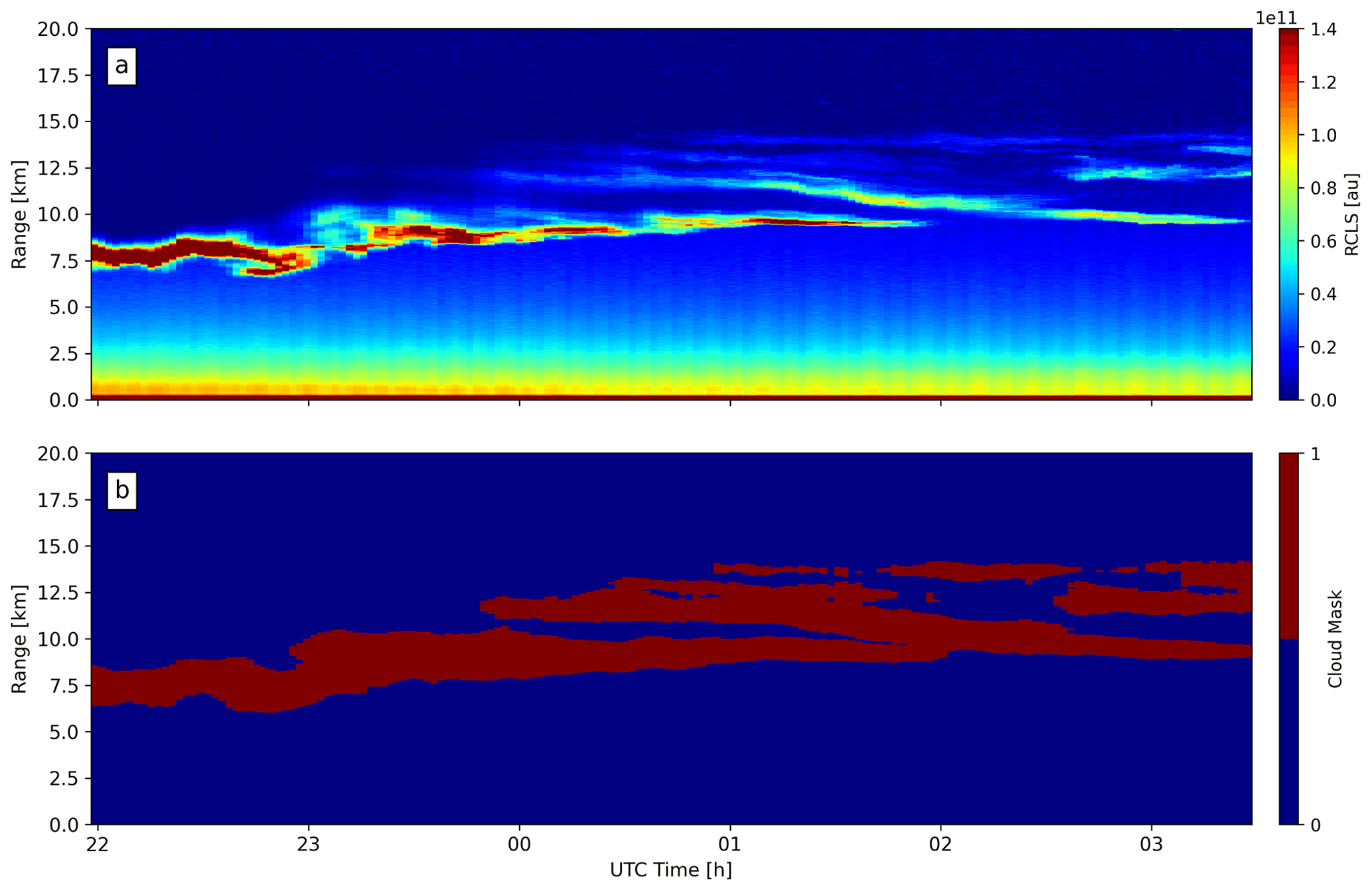
Figure 9 (a) RCLSs and (b) cloud layer mask for the Manaus lidar station from 22:00 UTC on 14 August 2011 to 03:30 UTC on 15 August 2011.

For the retrieval of the optical properties, we used a lidar ratio of 23.3 sr following the measurements reported by Gouveia et al. (2017b). Figure 10 shows the particle extinction profile at 02:15 UTC (5 min average). While there seem to be three layers of cirrus clouds, the structure is quite complex, and none of the layers are isolated. The corresponding cloud optical depth is 0.46, which is large enough for multiple scattering to be important, but this has not been accounted for. Nonetheless, the extinction values and the cloud optical depth (COD) are reasonable and in the typical range of previous works (Gouveia et al., 2014, 2017b), and they show what can be obtained with the current version of the LPP.

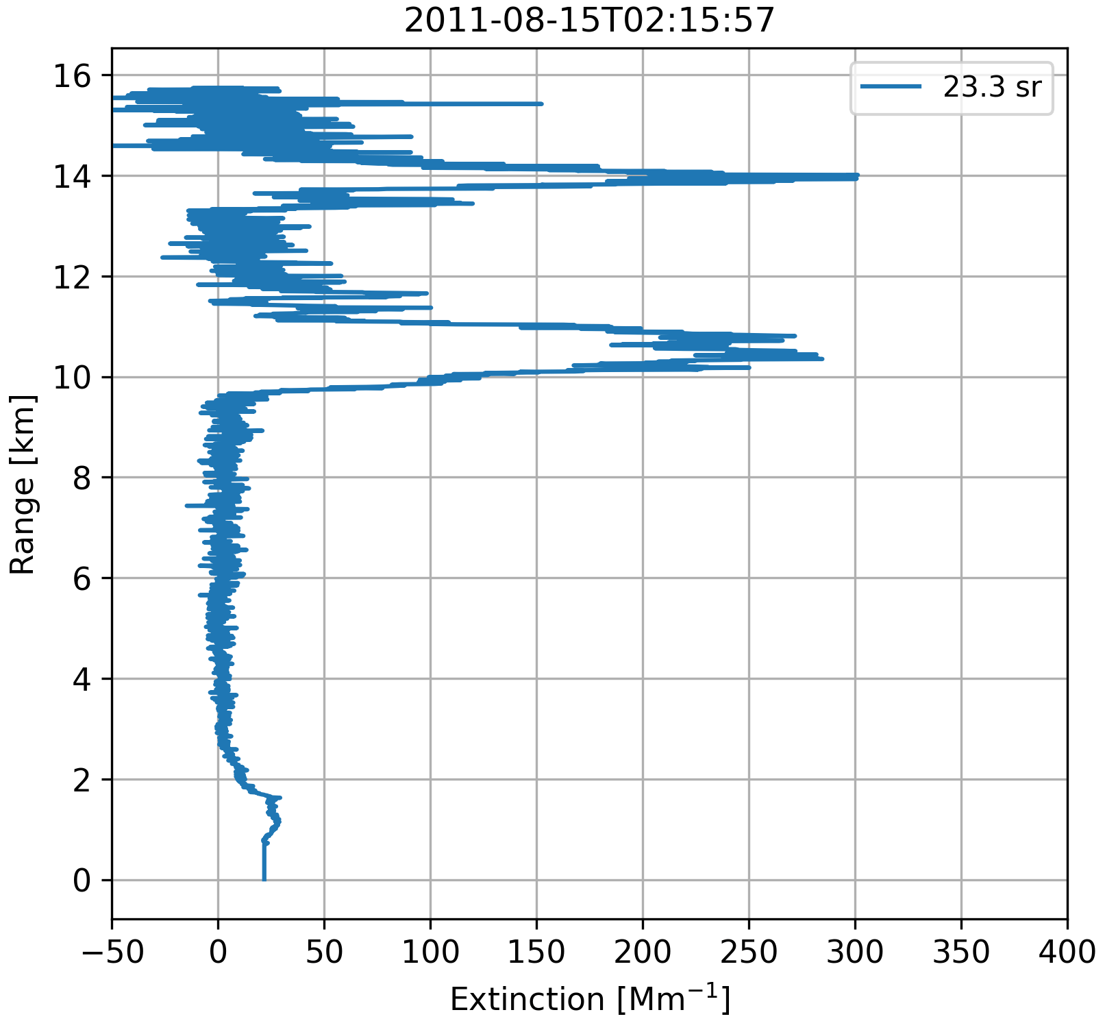
Figure 10 Extinction coefficient obtained using a constant lidar ratio of 23.3 sr for the cirrus clouds over the Manaus lidar station from 02:15 to 02:20 UTC on 15 August 2011. The extinction coefficient was assumed constant below 750 m.

4.5 Future roadmap

With the first release of the LPP and its use by the different groups in LALINET, we have identified the necessary improvements and built a roadmap to guide future development. An initial consideration is that the LPP-processed data files must be FAIR (findable, accessible, interoperable, and reusable) (Wilkinson et al., 2016) to be compatible with open science. In this sense, more information about the site, hardware, operation, files processed, and even the version of the LPP used needs to be added as metadata in the output files. Moreover, the benefit of the LPP's highly modular concept is the possibility of different groups modifying and testing different modules without interfering with the rest of the pipeline. To facilitate the customization of the pipeline to fulfill different needs and to allow more groups to contribute to the LPP's development, future releases will include Python versions of all modules.

In terms of improvements in the physical retrievals, we have identified three priorities. The first is to implement the Klett (1985) solution in the lidar equation with a range-dependent LR. This would be useful, for instance, for the São Paulo station, where the sea breeze frequently brings marine aerosols above the urban-polluted boundary layer (Rodrigues et al., 2013; Ribeiro et al., 2018). The second is to obtain the uncertainties in the extinction and backscatter coefficients by propagating the signal errors using a Monte Carlo approach (Press, 2007), following the work of Alvarez et al. (2006) and Mattis et al. (2016). Finally, we plan on implementing the Raman solution (Ansmann et al., 1992), but this might require an intercomparison effort of the existing algorithms in LALINET, as was done in EARLINET (Pappalardo et al., 2004). Moreover, in LALINET, the stations recording Raman return signals have photon-counting channels, which might be affected by dead-time effects (Johnson et al., 1966). Hence, we need to implement the known dead-time corrections for paralyzable and non-paralyzable systems (Whiteman et al., 1992; Knoll, 2010), which would also allow for “gluing” of the analog and photon-counting channels to extend the instrument dynamic range (Whiteman et al., 2006; Newsom et al., 2009).

Regarding the automation of the pipeline, a few updates are planned. For instance, we noticed that only a few lidar stations in Latin America have a nearby radio-sounding site, and they are launched once or twice per day. To facilitate the processing of level 1 and level 2 data, an automatic “thermodynamic profile downloader” will be developed to obtain a co-located thermodynamic profile from a nearby radio sounding, a forecast model, or a reanalysis. The MPLNET data processing, for example, automatically retrieves meteorological profiles from the Goddard Earth Observing System, version 5 (GEOS-5) atmospheric general circulation model for all molecular calculations (Lewis et al., 2016). We also plan to implement a method of rescaling the standard atmosphere profiles based on co-located ground-based temperature and pressure measurements, which could also be retrieved automatically from meteorological databases.

Moreover, a well-known problem with the inversion of elastic lidar data is the need to assume an a priori lidar ratio. The typical solution is to choose a lidar ratio that brings the estimated AOD value closer to the reference value measured by AERONET, which can now be measured during the daytime and nighttime (Perrone et al., 2022). This analysis can be made a posteriori, as shown in Fig. 8. Implementing an optimization routine would allow the LPP to automatically identify the best LR for each profile, as has been done in previous studies (Córdoba-Jabonero et al., 2011; Román et al., 2018), and help reduce systematic errors in the retrieved profiles (Welton and Campbell, 2002). The user could provide the reference AOD value, or it could be obtained by an “AOD data downloader” tool as part of the LPP framework.

5 Conclusions

Lidar networks are drivers of scientific advancement as they coordinate the efforts of different groups, allowing for uniform quality-assurance procedures, as well as instrument comparison and algorithm validation. The development of the LPP is a joint effort leveraging the expertise and personnel of different Latin American lidar groups that are part of the Latin American Lidar Network. The goal of the LPP is to provide a set of open-source tools for each step of the typical lidar data analysis routine. Here, we provide a high-level overview of the first working version, which is now released for the scientific community on our GitHub repository.

The performance of the LPP was evaluated through an analysis of synthetic and measured elastic lidar signals. For noiseless synthetic signals with a constant LR, the mean relative error in the aerosol extinction within the boundary layer was quite small, ranging from −0.005 % to −0.9 %, depending on the wavelength. For noisy synthetic signals with a variable LR, the mean relative error in aerosol backscatter was larger, ranging from −0.63 % to 4.5 %, mostly due to assuming a constant LR in the inversion. For the case studies for urban aerosols in São Paulo and cirrus clouds in the Amazon, we found LR and COD values, respectively, in agreement with previous results. These analyses showed the capabilities of the current release but also highlighted the need for new features. Hence, we have built a roadmap to guide future development, which includes (1) improvements in the physical retrievals (e.g., range-dependent LR inversion of the elastic signal or uncertainty propagation using Monte Carlo) and (2) automation of the pipeline (e.g., optimizing the elastic LR by constraining the column AOD or thermodynamic profile downloader tools). Future releases will bring these and other new features, accommodating the needs of our community.

Although the scientific community is moving towards open science, developing open-source code is still a hurdle, and the atmospheric lidar community has not yet fully embraced the idea. Consolidated networks have long developed their own algorithms and pipelines, which unfortunately remain mostly inaccessible to the community, hampering faster scientific advancement. We hope open-source efforts, such as the one presented here, become the rule rather than the exception in the near future.