the Creative Commons Attribution 4.0 License.
the Creative Commons Attribution 4.0 License.
 | 15 Sep 2023
Verification and calibration of a commercial anisotropic magnetoresistive magnetometer by multivariate non-linear regression
Mary Knapp
Rebecca Masterson
Cadence Payne
Kristen Ammons
Frank D. Lind
Kerri Cahoy
Commercially available anisotropic magnetoresistive (AMR) magnetometers exhibit on the order of 1 nanotesla (nT) sensitivity in small size, weight, and power (SWaP) packages. However, AMR magnetometer accuracy is diminished by properties such as static offsets, gain uncertainty, off-axis coupling, and temperature effects. This work presents a measurement of the magnitude of these effects for a Honeywell HMC1053 magnetometer and evaluates a method for calibrating the observed effects by multivariate non-linear regression using a 24-parameter measurement equation.
The presented calibration method has reduced the vector norm of the root mean square error from 4300 to 72 nT for the data acquired in this experiment. This calibration method has been developed for use on the AERO (Auroral Emissions Radio Observer) and VISTA (Vector Interferometry Space Technology using AERO) CubeSat missions, but the methods and results may be applicable to other resource-constrained magnetometers whose accuracies are limited by the offset, gain, off-axis, and thermal effects that are similar to the HMC1053 AMR magnetometer.
- Article
(1515 KB) - Full-text XML
- BibTeX
- EndNote


1.1 Satellite magnetic sensing
Magnetic sensing is used on satellites for orientation determination in low Earth orbit (LEO) and for scientific observations of planetary bodies and solar wind (Albertson and Van Baelen, 1970). Earth's surface magnetic field is dominated by the dipolar mode (or component), but spherical expansion representations of Earth's magnetic field can define global magnetic maps which achieve vector component accuracies of about 150 nT and angular accuracies of about 1∘. Such maps include the World Magnetic Model (Chulliat et al., 2020) and the International Geomagnetic Reference Field (IGRF; Alken et al., 2021). If a satellite magnetometer can achieve similar measurement accuracy, then the magnetic attitude determination accuracy will be primarily limited by map models and not magnetic sensing. This level of accuracy would enable magnetic-only attitude determination and control, in which a satellite senses its orientation with a vector magnetometer and controls its orientation without the use of reaction wheels or control thrusters and instead uses only magnetorquers for actuation (Liu et al., 2016).
Additionally, magnetometers are used for the scientific observation of solar system bodies (Russell et al., 2016), solar wind (Horbury et al., 2020), and other space weather events (Kletzing et al., 2013). Satellite-borne magnetometers provide information about planetary geology by measuring the magnitude, orientation, and variation of an object's magnetic field (Leger et al., 2009). On solar system objects without an internally generated dynamo field, the crustal remnant magnetic fields still provide information on the body's history and composition (Connerney et al., 2015). Magnetic field observations are also used to learn about the space plasma environment, such as the connection between planetary magnetic fields and solar coronal activity (Nicollier and Bonnet, 2016).
1.2 Anisotropic magnetoresistive (AMR) magnetometers
Materials with magnetoresistance exhibit a variation in the electrical resistance with the incident magnetic field. Some materials exhibit a sub-type of magnetoresistance in which the change in the resistance depends also on direction of the applied magnetic field and not just the magnitude (Gu et al., 2013). Anisotropic magnetoresistive (AMR) magnetometers utilize this effect by converting the change in the material resistance into a measurement of the direction of the applied magnetic field. With a four-element Wheatstone bridge configuration of the AMR material, AMR magnetometers produce an analog output approximately proportional to one vector direction of the magnetic field (Ripka et al., 2003). This configuration is used by the Honeywell HMC model series discussed in this work.
The AMR materials in an AMR magnetometer can be deposited as a thin film on silicon and therefore integrated into small electrical components with dimensions on the order of a few millimeters per side. Furthermore, these packages can contain three perpendicular devices that enable the simultaneous and independent measurement of three orthogonal magnetic field vector components. Such components that integrate three-axis AMR sensing into one unit include the Honeywell HMC1053 and the Memsic MMC5603MJ. The Honeywell HMC1053 has been selected for study in this work and was selected for use on the AERO (Auroral Emissions Radio Observer) and VISTA (Vector Interferometry Space Technology using AERO) CubeSats for properties such as low electrical noise, due to analog design and steady-state operation, low SWaP (small size, weight, and power), and component family flight heritage on similar CubeSats such as ANDESITE (Ad-hoc Network Demonstration for Spatially Extended Satellite-based Inquiry and Other Team Endeavors), as described by Parham et al. (2019), and CINEMA (CubeSat for Ions, Neutrals, Electrons, and Magnetic fields), as described by Archer et al. (2015).
1.3 Motivation
The AERO and VISTA missions use two low Earth orbit 6U CubeSats to perform scientific observation of radio emissions from the Earth's aurora and other high frequency (HF) signals at radio frequencies from 100 kHz to 15 MHz (Erickson et al., 2018; Lind et al., 2019). To contextualize the radio frequency measurements, the AERO and VISTA spacecraft will also contain low-SWaP magnetometers with an accuracy better than 100 nT (Belsten, 2022). These magnetometers will measure auroral current systems as the spacecraft passes through, providing scientific context for the radio frequency observations gathered by the radio frequency vector sensor antenna. The precision and noise floor of the HMC1053 magnetometer analyzed in this work meets the mission measurement requirements, but the manufacturer's data sheet also reports inaccuracies due to a number of effects, including temperature dependence, off-axis coupling, constant offsets, uncertain gains, and non-linearity.
In orbit, AERO–VISTA will use GPS and star tracker for absolute measurement of the spacecraft's position and orientation. This will be used with global magnetic maps to determine the magnetic field in the spacecraft reference frame. The vector magnetic field in the spacecraft body frame will be used as a calibration source for the AERO–VISTA mission. This work evaluates the expected accuracy achievable with the AERO–VISTA magnetometers and the associated calibration method, but we do not intend to use ground-derived calibration parameters in orbit. For the data collected on the ground, the proposed model achieves a root mean squared (rms) fitting error compared to a reference magnetometer of better than the mission requirement of 100 nT rms. This calibration is achieved under the expected field range of ±50 µT in all axes and over 35 ∘C temperature range. Limitations in data collection on the ground have resulted in incomplete parameter fitting, as discussed in Sect. 3.2. However, we did successfully fit the x-axis data over a range of magnetic field and temperature variations with adequately low rms error, which serves to verify the performance of this combination of hardware design and calibration method. Given this result, AERO and VISTA will use and further evaluate this magnetic sensing method in orbit, where the reference magnetic field for the parameter fitting will be provided by global magnetic maps when the spacecraft is at low latitudes.
1.4 Magnetic calibration methods
Magnetometer calibration involves modeling and estimating the errors reported by a magnetic sensor. With an accurate model, the expected error of the sensor can be predicted and subtracted for a more accurate overall measurement (Hadjigeorgiou et al., 2020). Often, scalar magnetometers can achieve greater scalar accuracies than vector magnetometers, so they can be used as a calibration source for vector magnetometers. Particularly for rotating platforms, the scalar reference can be used for a robust estimation of the vector calibration parameters, using methods such as the TWOSTEP algorithm (Alonso and Shuster, 2002) or Kalman filtering (Crassidis et al., 2005). These works develop attitude-independent calibration methods which do not use absolute attitude sensors. Other models can be fitted by using a least squares estimation (Gebre-Egziabher et al., 2006).
In the case of AERO–VISTA, an independent source of attitude is provided by the spacecraft attitude determination and control system (ADCS), namely the star tracker. This system provides absolute pointing information at better than 0.1∘ accuracy. Therefore, AERO–VISTA can derive the magnetic field in the spacecraft coordinate frame from global magnetic maps that are independent of any other on-board magnetic field sensors. This field will be used as a calibration reference for the mathematical model and least squares fitting in this work.
Previous works by Archer et al. (2015) and Parham et al. (2019) have verified the capabilities of commercial AMR magnetometers and also determined the calibration coefficients for parameters such as angular offset, gain uncertainty, and the temperature dependence of the offset. The work by Archer et al. (2015) uses attitude-independent methods to fit the calibration coefficients for the gain, offset, angular position, and temperature coefficients for the gain and offset, using in-orbit magnetometer data and the IGRF as a reference. The work by Parham et al. (2019) evaluates the gain, offset, and temperature coefficient of Honeywell HMC1001 and HMC1002 magnetometers using ground-based testing. This work describes the collection of ground data that is sufficient to verify the calibration performance by fitting coefficients for the gain, offset, off-axis coupling, and temperature coefficients for all terms. This work verifies the findings of the previous works to within the noise limit of the test magnetometer of about 20 nT. This work also applies previous CubeSat AMR magnetometer verification and calibration efforts to the HMC1053 magnetometer implementation for the AERO–VISTA mission. Finally, the non-linear calibration equation in this work includes second-order couplings such as the temperature coefficients of off-axis terms.
1.5 Interfering sources of magnetization
Material in the vicinity of the magnetometer can be magnetized and can contribute an additional magnetic field that is superimposed upon the environmental magnetic field which we desire to measure. In space, satellite materials may be magnetized by the spacecraft's own magnetorquer or magnetic fields from large current sources, such as battery-charging circuits. Different materials exhibit different levels of magnetic hardness, which is the tendency of the material to retain magnetization after a magnetic field is removed. Magnetic hardness can be parameterized by coercivity, which is the magnetizing field necessary to remove the internal magnetization of the material, or by the remanence, which is the amount of magnetization left after a magnetizing source is removed. Magnetically hard materials contribute a constant offset to the magnetic field, and magnetically soft materials distort and scale the magnetic field (Gebre-Egziabher et al., 2006).
Many large spacecraft performing magnetic science place their magnetometers on multi-meter-long booms to remove the magnetometer from interfering fields generated by the spacecraft, such as on the Cassini–Huygens mission (Dougherty et al., 2004). Such missions may also create detailed magnetic interference budgets maintained by a standing magnetics control review board (MCRB; de Soria-Santacruz et al., 2020). Small satellites, and CubeSats in particular, often do not have the system mass and volume budgets to allow for large deployables, although some CubeSats such as CINEMA do have meter-scale magnetometer booms (Archer et al., 2015). The magnetometer on AERO–VISTA is a secondary payload to the radio frequency sensor, so SWaP is even more limited. Therefore, the AERO–VISTA magnetometer is inside the 6U spacecraft bus and will be subject to interference from nearby materials. The interference from some materials can be calibrated out as offsets or sensitivity changes, as is developed in Sect. 3. If the material is neither magnetically soft nor magnetically hard, then it can introduce complex time-varying errors which depend on the history of magnetization of the system. These effects can also be created by properties of the magnetometer itself (Bernieri et al., 2007), so we undertake an investigation into the hysteresis of the magnetometer in Sect. 2.3.4.
The performance of the magnetometer or device under test (DUT) has been evaluated by simultaneously exposing both the DUT and a reference magnetometer to a variety of magnetic fields and temperatures.
2.1 Test hardware
An engineering development unit (EDU) for the AERO–VISTA magnetic sensing instrument was developed for this calibration experiment. The electronics in the EDU amplify, digitize, time stamp, and store the signals from the magnetometer and have been described in a previous work (Belsten et al., 2022). A Macintyre Electronic Design Associates (MEDA), Inc., FVM400 magnetometer is used as a ground truth magnetic measurement reference. A 3D-printed mechanical mount for the EDU constrains the DUT in space at about 1 cm distance to the reference magnetometer. By keeping a level of separation between the magnetic sensing instruments and any magnetized source, the magnetic gradients are minimized, such that the magnetic field at the DUT is the same as at the reference magnetometer to within the expected accuracy of the DUT (order 10 nT).
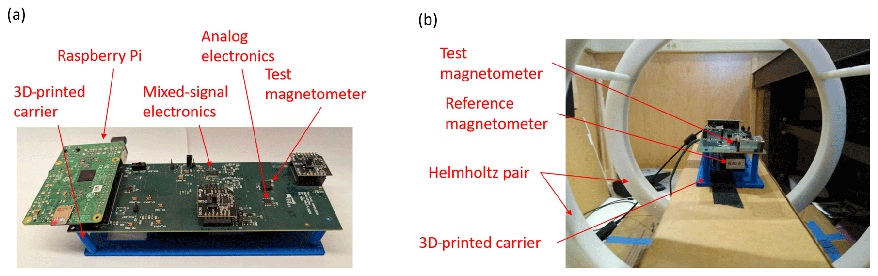
Figure 1Experimental setup for data collection showing the (a) magnetometer implementation and (b) testing configuration. Panel (a) shows the electronics system for operating and testing the HMC1053 magnetometer. Panel (b) shows the testing apparatus with the test and reference magnetometers placed within a Helmholtz coil for application of the external magnetic field.
For all experimentation, the MEDA FVM400 reference magnetometer is assumed to be a zero-error ground truth measurement. It is possible that some effects fitted by the calibration model are actually characteristics of the reference magnetometer and not the DUT, but assuming that all error belongs to the DUT and not the reference magnetometer is a conservative bounding assumption for an analysis of the DUT.
2.1.1 Magnetometer configuration and operation
The amplified analog signal from the HMC1053 is digitized at 20 samples per second (SPS). The analog-to-digital converter (ADC) contains a single ADC circuit with an eight-channel multiplexer so that the three axes and the temperature sensor are read sequentially. The duration of all sequential conversions results in a total effective sample period of 0.4 s. The HMC1053 magnetometer includes a set and/or reset polarity inversion functionality to correct for large offsets and to reduce hysteresis effects (Ripka et al., 2003). This switching offset calibration operation is used during data collection for this work, as described for the AERO–VISTA engineering and flight models in a previous work by Belsten et al. (2022). Therefore, only the offsets remaining after the set and/or reset polarity inversion are considered in our calibration method (discussed in Sect. 3).
The FVM400 reference magnetometer samples at four samples per second. The magnetic measurement data from the two magnetometers are compared using interpolation to the four SPS rate of the reference magnetometer. The effects of any sampling offset in time are discussed in Sect. 2.2.
2.2 Test environment
All testing reported in this work was performed in a magnetic test facility which contains steel magnets embedded in the walls, ceiling, and floor, which are oriented to cancel out the environmental magnetic field within a large volume. This magnetic field is most uniform away from the edges of the facility. This facility does not cancel out time-varying magnetic fields by human-produced noise or space weather, although care is exercised to keep sources of magnetism away from the facility. Typical magnetic noise in this location exhibits a peak-to-peak amplitude of 0.3 µT, with most power at frequencies below 1 Hz (Belsten, 2022). The test and reference magnetometers operate simultaneously to within the resolution of the sample periods; therefore, environmental variations in timescales that are slower than the about 0.5 s sample period will not affect the measurement comparison. A measurement simultaneously showing uncalibrated test magnetometer (DUT) and reference magnetometer measurements of the environmental magnetic noise is shown in Fig. 2a.

Figure 2Evaluation of the magnetometer constant offset using a near-static magnetic field. The simple offset calibration calibrates to the noise floor for the data collected in this location, as seen in the flat profile in panels (c) and (d). Panel (a) shows simultaneous raw measurements from the test and reference magnetometers. Panel (b) shows data from panel (a) but with the constant offset subtraction applied to the test magnetometer data. Panel (c) shows the difference (delta) between the raw test and reference magnetometer over time. Panel (d) shows the delta between the test and reference magnetometer measurement with the static offset subtracted.
2.3 Data collection and performance verification
Using the hardware described in Sect. 2.1, the magnetic errors of the DUT due to non-ideal effects have been measured. We use the magnitude of these impacts to determine which non-ideal effects need to be included in the calibration model in Sect. 3. Data were collected in the lab to evaluate the effect of each anticipated source of inaccuracy, as follows:
-
constant offset in each axis
-
gain error in each axis
-
non-orthogonality and misalignment (off-axis coupling)
-
temperature dependence of each of the above parameters
-
hysteresis
-
non-linearity.
2.3.1 Constant offset
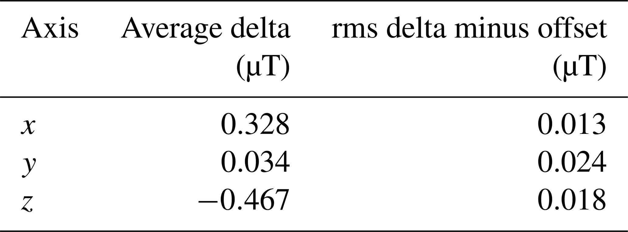
The constant offset was tested by placing the measurement device in the low-magnetic-field room (minimizing the effects of gain uncertainty) and collecting simultaneous data for 2 min. The raw measured field is reported in Fig. 2a; the average offset for each axis is subtracted from the DUT measurement and shown in Fig. 2b. The offset variation in time is shown in Fig. 2c, and the residual difference after the average offset is subtracted is shown in Fig. 2d. The average difference between the measurement of each axis and the root mean square (rms) residual error is reported in Table 1.
Table 1Average offset fit for each axis and the residual root mean square (rms) error.
2.3.2 Single-axis applied field
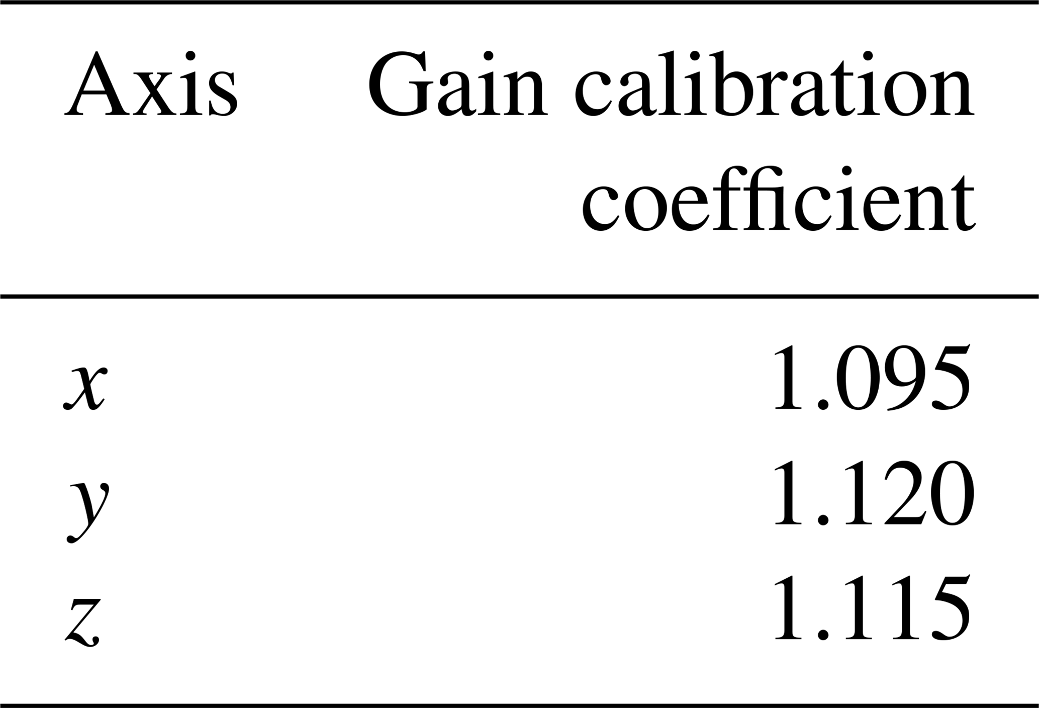
A single-axis applied field experiment was conducted for each orthogonal orientation in which the incident magnetic field was stepped from −50 to 50 µT. The regression to the data collected in these experiments yields the gain calibration coefficients reported in Table 2. The data collected in these experiments are also used to determine the off-axis coupling in the full calibration model described in Sect. 3. Additionally, by stepping these measurements through several increments during testing, we have screened for non-linearity in the magnetometer, as seen in Fig. 3. The measurements and calibrations demonstrated in Fig. 3 were repeated for the y axis and z axis. All three axes show a flat calibrated line once the linear calibration is applied, indicating that the instrument does not exhibit observable non-linearity within the measurement noise floor.
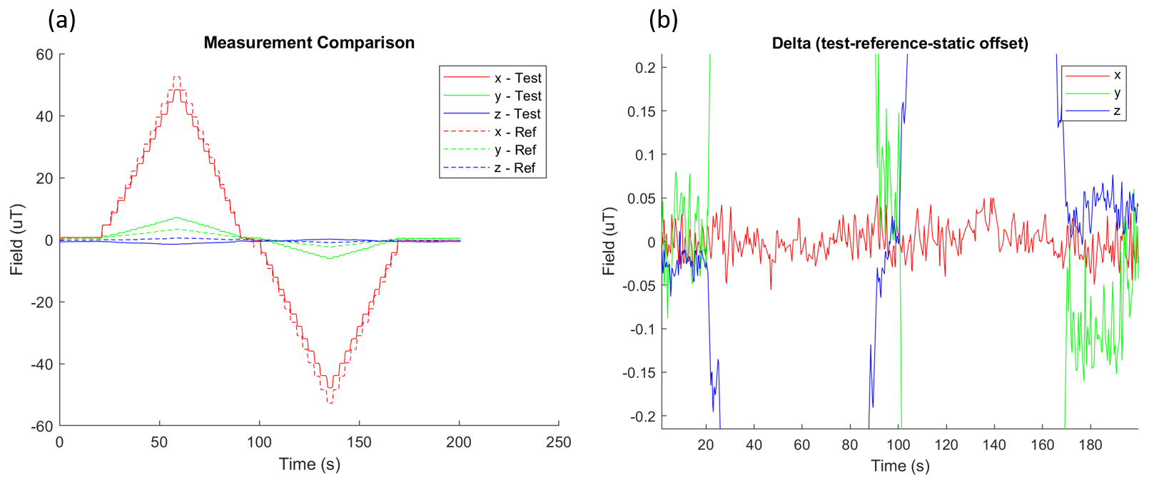
Figure 3Data capture for the evaluation of the gain and linearity of the x axis. Panel (a) shows the non-calibrated magnetic measurements while stepping the x-axis-applied field. The data in panel (a) are calibrated using a linear slope and an offset fit to yield panel (b). The flatness of the calibrated curve in panel (b) indicates that linearity errors are not observable with the current noise floor.
Table 2Gain calibration coefficients for x, y, and z axes, as determined by the linear fit during single-axis incident field tests.
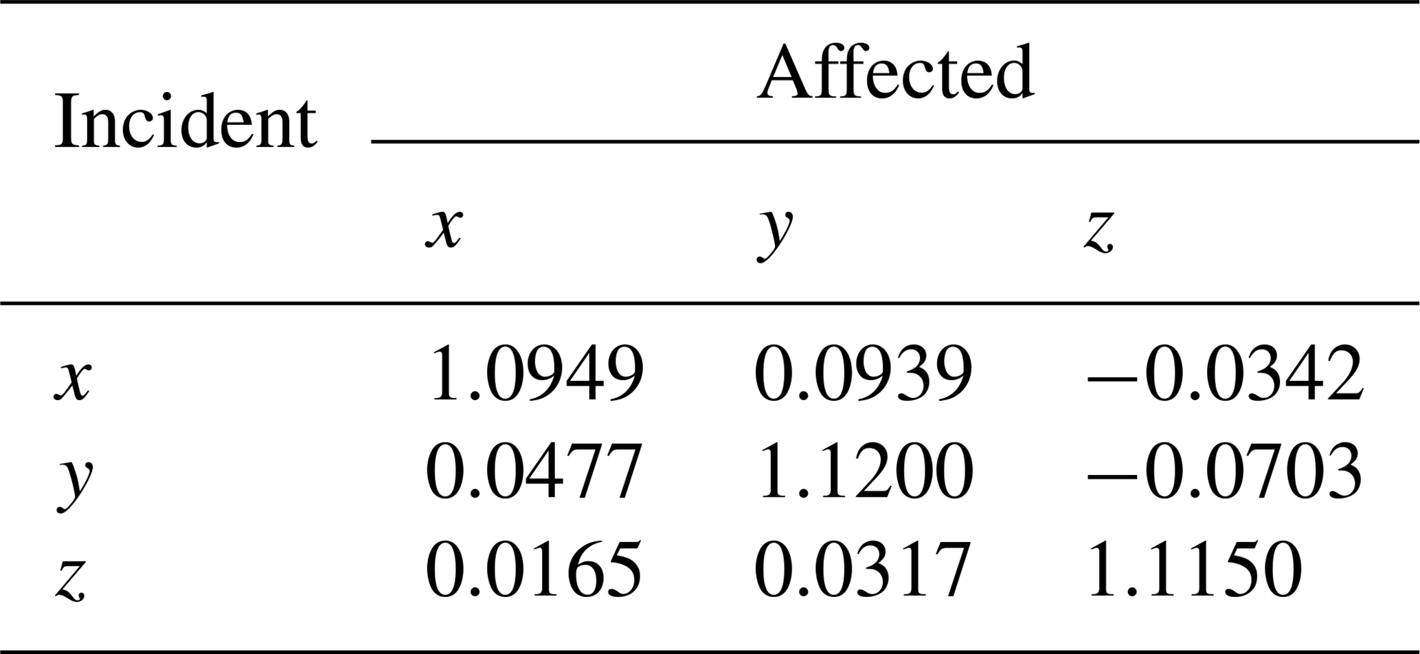
The off-axis effects are analyzed with the data collected during the single-axis measurements. Some off-axis coupling is expected due to the residual misalignment of the magnetic-field-inducing coil with the magnetic field measurement system. However, this alignment error is the same for the test and reference magnetometers, so the differences between the test and reference magnetometers contain information about the off-axis couplings of the magnetometers themselves, which are assumed to be inherent to the DUT. The fit to the off-axis coupling is reported in Table 3
2.3.3 Temperature effects
In this test, the circuit board with the DUT was heated to about 65 ∘C and allowed to cool to a steady state – approximately a 30 ∘C temperature range – while capturing magnetic field data. During this experiment, a constant magnetic field was applied along the x axis to evaluate the change in the gain coefficient due to the temperature change. The measured fields over temperature are reported in Fig. 4. The linear fit to the x-axis data in Fig. 4 derives a linear temperature coefficient of −140. nT ∘C−1.
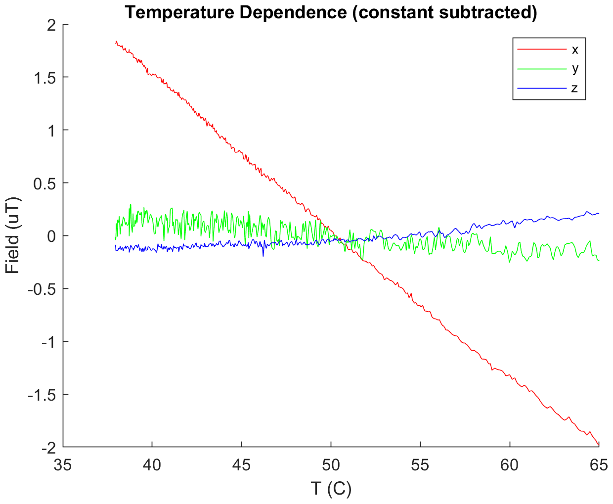
Figure 4Temperature variation with a magnetic field applied along the x axis primarily shows along-field measurement variation, but a variation is also observed to a lesser degree in the off-axes terms.
2.3.4 Hysteresis
Hysteresis effects are difficult to calibrate, as they require knowledge of the past states of the magnetic environment. The magnitude of hysteresis effects was measured by applying the maximum expected incident magnetic field – which in the case of AERO–VISTA is set by the magnetometer's proximity to the spacecraft magnetorquers and is 150 µT. This maximum field is applied in the positive and negative directions. After the application of the magnetizing field in each direction, the magnetizing field is zeroed, and the difference between the measured magnetic fields after the two extreme magnetizing field polarities estimates a worst-case error due to hysteresis. The data collected for this test are shown in Fig. 5. The reference magnetometer shows about 0.47 µT of the remanent field difference, and the test magnetometer shows an additional 50 nT of the remanent field. Given that both magnetometers reported similar hysteresis effects, the source of the hysteresis is likely the magnetization of the material near both magnetometers and not an effect inherent to either magnetometer alone (one likely source is the connectors on the Raspberry Pi, which will not be present in the AERO–VISTA flight model). This observation indicates the need to maintain magnetic cleanliness close to the magnetometer. The 50 nT difference in hysteresis between the test and reference magnetometer is attributable either to a gradient in the magnetic field caused by the source of interference or is inherent to our magnetometer instrument – or some combination of both. Given that our requirement is 100 nT, we consider this to be an acceptably low sensor hysteresis even if all observed hysteresis is attributable to the instrument effects. For a discussion of the strategies for magnetic cleanliness on AERO–VISTA, see the work by Belsten (2022).
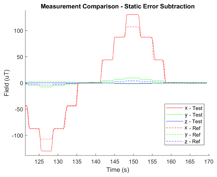
Figure 5A positive and negative 150 µT magnetic field excursion is used to screen for hysteresis effects.
2.4 Summary of observed accuracy effects
Table 4 summarizes the error magnitude of each of the effects analyzed. Where there may be multiple instances of such a measurement (multiple axes, for example), only the worst-case value from the measurements in Sect. 2.3 are reported in Table 4.
Table 4Summary of the measured non-ideal properties. This information has been adapted from Belsten (2022).
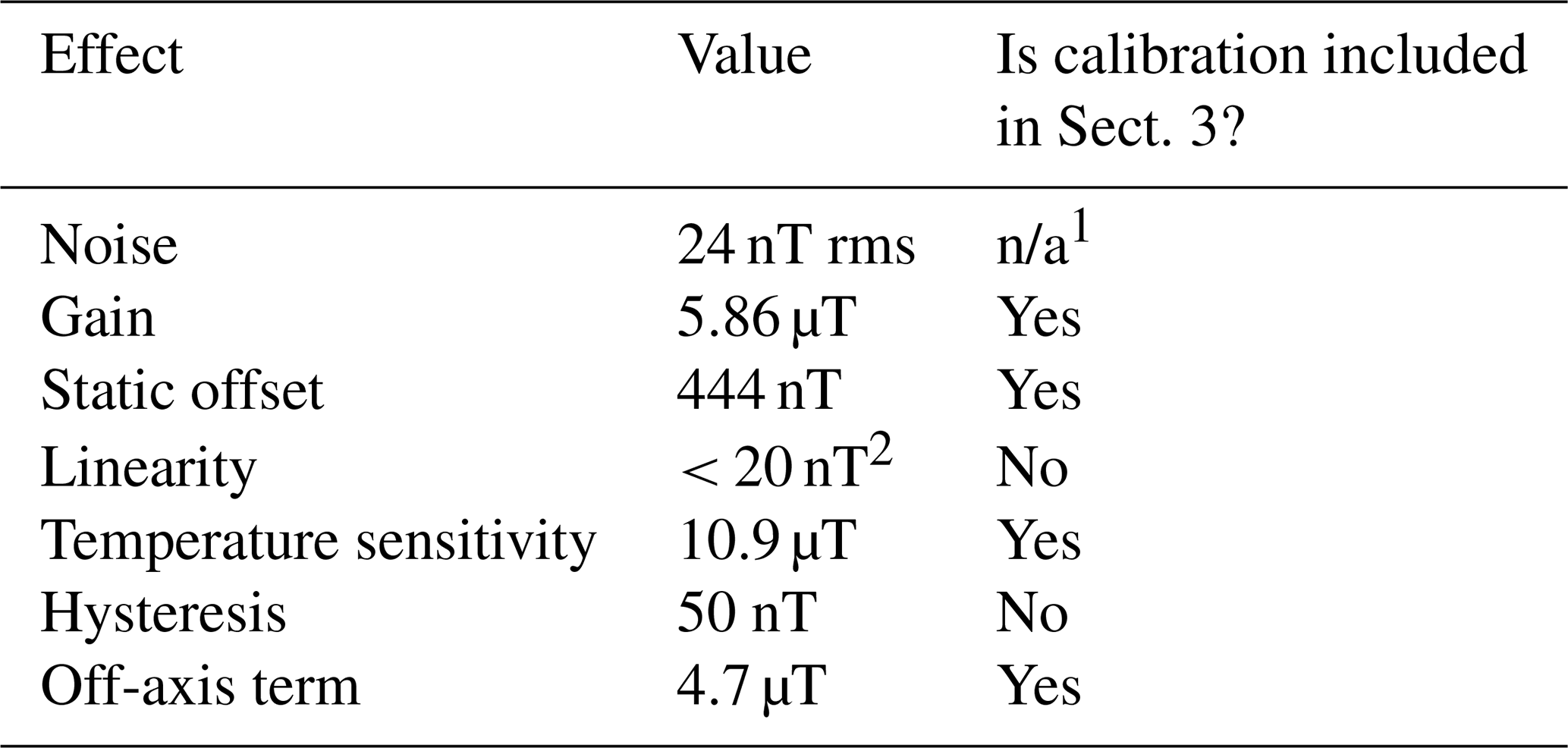
1 Calibration is not applicable (n/a) to noise. 2 Linearity was not observed within the noise floor of this experiment.
2.4.1 Second-order terms
Table 4 reported each of the major interfering terms but did not consider the combination of multiple effects (e.g., how the static offset varies with temperature). The effect of second-order terms was estimated by combining their fractional effect when compared to the full-scale measurement. The largest first-order effects from Table 4 are combined to estimate the contribution, as reported in Table 5.
Table 5Second-order non-ideal effects as evaluated by combining the fractional contribution of each first-order effect. This information has been adapted from Belsten (2022).
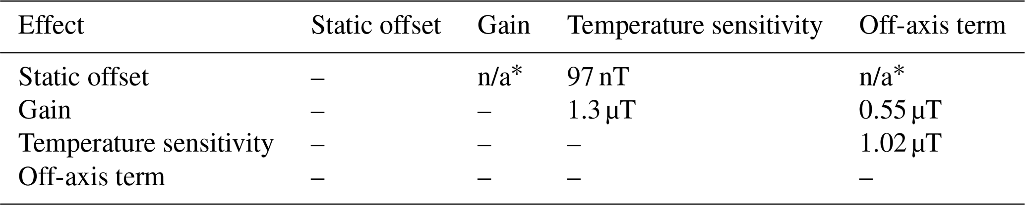
* The static offset contribution does not change with applied field, so the combination of offset with gain and off-axis fields is not applicable (n/a).
This work utilizes a mathematical function to model the observed non-ideal parameters of the magnetometer. Commonly, this function incorporates a 3×3 matrix for gain and a three-vector constant offset to characterize both the instrument and the attitude of the instrument with respect to a reference magnetic field.
The matrix C can represent many physical operations, such as the coordinate frame rotation (as is done for attitude-independent methods; Alonso and Shuster, 2002), non-orthogonality, misalignment, and scaling (Soken, 2018). Outside of the instrument itself, soft iron errors also create off-axis terms in the same sensitivity matrix (Elkaim, 2002). Each of these effects can be parameterized with their own structured matrix (see, for example, Soken, 2018). The rightward multiplication of all leading matrices results in one final 3×3 matrix in our calibration equation, which accounts for the combined effects of misalignment, non-orthogonality, scaling, and soft iron interference. During operation, we need the calibrated magnetic instrument to predict accurate environmental magnetic fields from what is measured by the magnetometer; so, to achieve a minimum rms error, it is desirable to perform least squares fitting on the reference magnetic field and not on the instrument-measured magnetic field. We achieved this by rearranging Eq. (1) to write Bact as the dependent variable and Bmeas as the predictor. Now we have Eq. (2).
In the new formulation, the sensitivity matrix S is related to the previous by and . Due to the strong temperature dependence observed for the gains and offsets in the experiments in Sect. 2.3, we include temperature terms for all parameters in the reformulated sensitivity matrix and for the offset to arrive at Eq. (3). This equation also maps to the individual effects observed in the series of individual linear fits described in Sect. 2.3 and summarized in Tables 4 and 5. Other alternative measurement equations could be considered, as we discuss in Sect. 3.4.
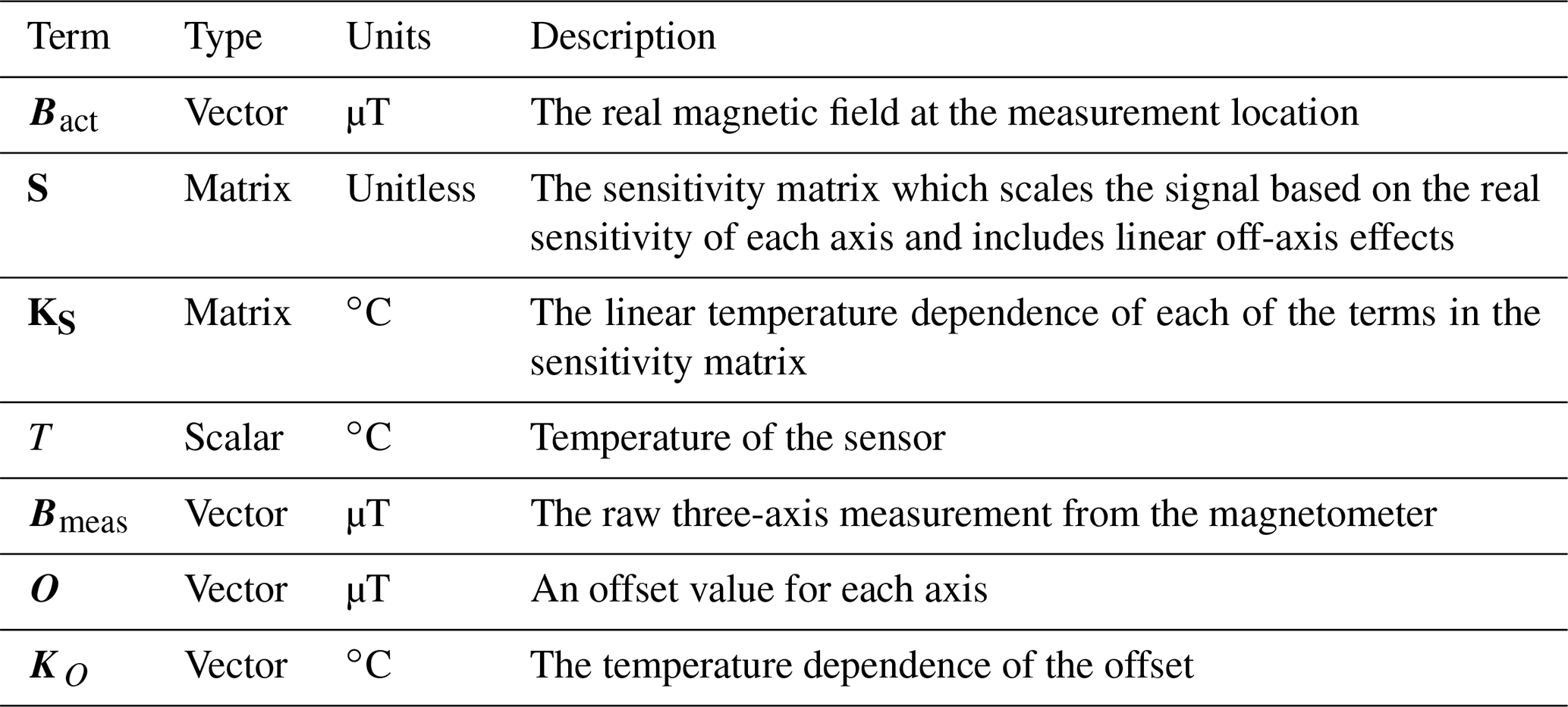
The parameters in Eq. (3) are defined in Table 6. The calibration is applied by using the reference magnetometer data as Bact and the test magnetometer data as Bmeas. Regression is applied on the thousands of data points collected across incident magnetic field and temperature conditions. The results shown in this work have used the MATLAB fitnlm function to implement a non-linear regression with a separate eight-element model for every fit parameter; however, the model is easily implemented with other non-linear regression fitting functions in other languages, such as Python's scipy.optimize.least_squares. Once the parameters are found, they can be used to find the calibrated magnetic field Bact for future measured fields Bmeas simply by solving the equation algebraically.
3.1 Calibration result
The fit of the calibration equation has been evaluated by applying the entire calibration model to all data collected in the determination of the non-ideal effects, as described in Sect. 2.3 (except for the hysteresis measurement data, which saturated the reference magnetometer). The results of this regression are provided in Table 7.
Table 7Derived regression coefficients from combined data collection in Sect. 2.3.
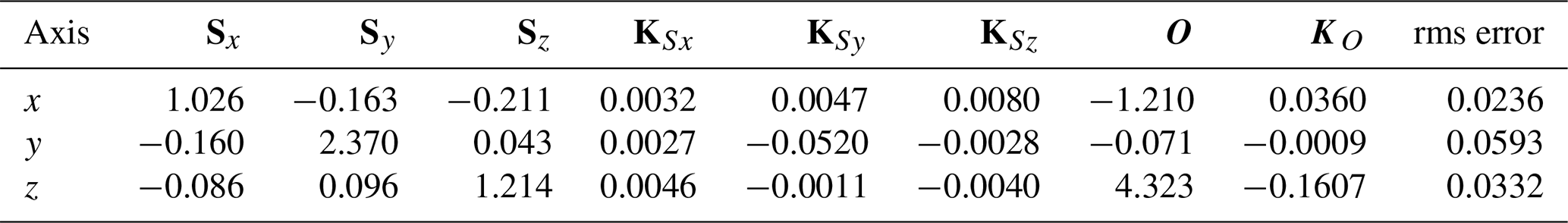
The magnetic field root mean square error for all axes is less than 60 nT, compared to the environmental noise of about 20 nT, as reported in Table 1. The observed error is marginally larger than the environmental noise floor of the instrument, so there are still impacts to the observed inaccuracy beyond simple noise. However, the rms error in the model fit observed in this ground experiment is sufficient to meet the AERO–VISTA measurement requirement of 100 nT.
3.2 Limitations
The data collection for the calibration verification in Sect. 2.3 has been limited by incomplete access to test facilities with the capability to generate arbitrary, low-noise, and accurate magnetic fields. A facility with a large magnetically shielded volume and precision three-axis Helmholtz coil would undoubtedly improve the accuracy of the calibration achieved on the ground. However, the fit errors achieved in this work are sufficient to meet the AERO–VISTA requirements, and the sequence of measurements in Sect. 2.3 can serve as a reference for future small satellite missions which aim to perform ground-based commercial magnetometer verifications with limited test facilities.
Importantly, due to the time-intensive and manual nature of setting up each measurement, the calibration reference data do not uniformly sample across magnetic field angles and across temperature. Thus, AERO and VISTA will likely encounter much greater data coverage in orbit as they rotate through Earth's magnetic field and naturally change temperature due to the orbital motion in and out of eclipse. In particular, the calibration data set in this work does not contain simultaneous perturbations of fields along the y and z axes of the magnetometer while the temperature is changed. This has resulted in the degeneracy of the fit, as discussed more in Sect. 3.3. Similarly, the magnetometer accuracy has not been evaluated at temperatures below room temperature, due to the difficulties in achieving cool temperatures without magnetic interference.
Other factors limit the maximum achieved accuracy due to limited measurement fidelity. The apparent source of the magnetic interference identified in the hysteresis test in Sect. 2.3.4 indicates that the reference magnetometer and test magnetometer are in the presence of a source of magnetic interference which could be changing with the incident field. If this is a purely soft or hard iron error, then it should be calibrated out, as discussed in Sect. 1.5; otherwise, this effect will cause differences in the actual magnetic field at the test and reference magnetometer. Other similar sources of error are non-uniformity within the generated magnetic field, time-varying magnetic gradients generated by magnetic noise, or mutual coupling of magnetic fields between the test and reference magnetometer. Each of these effects are artifacts of the ground testing infrastructure, which will not be present in orbit and only increase the rms error results reported in Table 7. Therefore, these effects do not invalidate the rms error findings as an upper bound for magnetometer accuracy performance.
3.3 Discussion
The results of the full model calibration are generally consistent with the individual parameter fits from Sect. 2.3. The offset values themselves and their temperature dependence are similar to the linear fit values from Sect. 2.3. Important exceptions involve the temperature terms for the y and z axes. For example, the diagonal components of the sensitivity matrix are near unity, with the exception of Syy, which can be explained by the sensitivity matrix temperature dependence, in particular for the diagonal terms of KS. The KSyy term is also anomalously large at −0.052 as compared to less than magnitude 0.01 for all other sensitivity terms. Most, but not all, measurements were taken at room temperature of approximately 25 ∘C, and using this temperature with the Syy and KSyy terms finds a room temperature y-axis sensitivity of 1.07, which is approximately unity, as expected. A similar issue is likely present in the combination of the z-axis O and KO terms, where, at room temperature, the combined O+KOT term is much nearer zero. This shows that a lack of characteristic calibration data can cause overfitting due to the degeneracy of the fit to the available data. Due to this limitation, the calibration parameters in Table 7 for the y and z axes would likely not perform well on a more varied data set that included the temperature excursion with incident fields applied along the y and z axes. More strictly, it would be beneficial to have data that uniformly cover the range of environmental conditions to avoid excessive fitting on clusters of data. Archer et al. (2015) perform such an analysis of orbital data by binning the attitude sphere into 192 equal-area bins and observing the fraction of bins with data points in them (Archer et al., 2015). This idea can be extended to cover the temperature variability by adding a temperature dimension with its own bins for each of the attitude bins and then counting the data coverage.
This limitation does not apply to the x-axis results, as the x axis was exposed to simultaneous variations in the temperature and incident magnetic fields in order to test the ability of our calibration model to accommodate such environmental changes. The successful fit of the x axis with a low rms error indicates that the physical processes that lead to the errors in the magnetometer can be calibrated with the proposed method. In the model equation, each response variable (the three-vector components of the measurement) is dependent only on its eight-variable subset of the entire equation. Therefore, the results achieved on the x axis in this experiment should generalize to the y and z axes.
The rms error results in Table 7 also validate the stability performance of the magnetometer hardware over time and power cycles. All data for the regression results in Table 7 were collected in 1 workday over several hours, with multiple system power cycles between different data acquisition activities. Stability on the order of hours is needed for AERO–VISTA operations, where calibrations only need to last for a few hours when calibration data acquired at low latitudes can be used during the same orbit for science acquisition at high latitudes.
3.4 Future work
This calibration method and magnetometer hardware will be evaluated in orbit with the data collected by AERO and VISTA. AERO–VISTA will use global magnetic models as a calibration source at low latitudes, where magnetic errors are at a minimum. In-orbit data may allow for the evaluation of the calibration method to a higher fidelity, since the magnetic measurements will not be affected by human-created magnetic noise and other limitations imposed by the experimental methods discussed in Sect. 3.2. The spacecraft bus may also generate noise, but the magnetic characterization of the bus during simulated spacecraft operation has found that bus-generated magnetic noise is less than about 20 nT rms (Belsten, 2022). This magnetic noise level is only achieved when the magnetorquers are not operating and has been kept to a minimum without a deployable boom by placing the bus electronics and magnetometer on opposite ends of the 6U spacecraft.
3.4.1 Calibration variation
All data collected in this experiment were obtained from one instrument during 1 workday over the course of several hours and a few power cycles. During the operation of the AERO–VISTA mission, we expect to obtain a sufficient range of calibration data during one orbit to robustly fit all calibration coefficients. However, it may be desirable to use calibration data from many orbits, possibly spanning days or months in time. This would be particularly true for calibrating out interference from the spacecraft, as discussed in Sect. 3.4.2. When calibrating on data obtained from many orbits, the variability in the device calibration coefficients with aging is important. Given the acceptable rms error results in Table 7 for the AERO–VISTA mission when using hours' worth of data, calibration stability is evidently not a problem on the timescale of hours with a few power cycles, but we do not yet know if it might be a problem over days or in the radiation environment of space. We do not anticipate investigating the longer-term stability of the magnetometer calibration coefficients on the ground, as it is not necessary for the core AERO–VISTA mission, but we do anticipate performing such an analysis with in-orbit data to provide results for future missions and to support further experimentation with AERO–VISTA, such as the interfering-source calibration discussed in Sect. 3.4.2.
Each spacecraft, AERO and VISTA, will have four magnetometers similar to the test magnetometer evaluated in this work. Therefore, the final AERO–VISTA mission will also serve as a comparison of the magnetometer calibration parameters unit-to-unit or within a production batch.
3.4.2 Calibration of spacecraft interference
Calibration by regression can be extended to account for major sources of interference if the interfering vector varies linearly with some measurable parameter. One such example is the current through a battery-charging circuit. The vector direction of the magnetic error at the magnetometer generated by this loop will be constant because the loop geometry is constant, and the magnitude will vary linearly with the current. Furthermore, AERO–VISTA (like most spacecraft) will collect housekeeping data on the current flowing through this loop. In general, these telemetry sources are not synchronized with the magnetometer sampling and are not at the same rate. In the case of AERO–VISTA, all telemetry is time stamped to 1 ms absolute accuracy; each parameter's telemetry rate only needs to sufficiently to capture the timescale of variability in the telemetry parameter for the calibration of interfering sources. For every such interfering-source current Ii, there is a vector sensitivity direction Di, such that the calibration equation Eq. (1) can be extended to Eq. (2), as discussed in Belsten (2022). The AERO–VISTA mission will attempt to improve the magnetic sensing accuracy by including some housekeeping data in the regression using Eq. (2).
3.4.3 Alternative calibration equations
We have reported on the reduction in the rms error by use of our calibration equation and regression, but future work should compare the performance of this calibration with other methods of calibration. Other variations on Eqs. (1) or (2) could be tried. For example, the temperature coefficients could be applied to Eq. (1) prior to reformulation to use the measured field as the predictor in Eq. (2). It would also be informative to evaluate how much accuracy is lost by the exclusion of some parameters of Eq. (3). This would allow for the simplification of the data collection and calibration pipeline at the expense of some accuracy performance. On the other hand, more parameters could be added to the calibration model, such as quadratic terms in gain or the cross-axis gain modulation effect reported by the manufacturer of the AMR magnetometers (Pant and Caruso, 1996). Alternatively, a machine-learning-based approach could be evaluated, as discussed, for example, by Styp-Rekowski et al. (2022).
This work evaluated the calibration of a magnetic sensor implemented with the HMC1053 anisotropic magnetoresistive (AMR) magnetometer manufactured by Honeywell. The accuracy degradation caused by the following parameters was evaluated using ground-based testing: constant offset and its temperature dependence, gain inaccuracy and its temperature dependence, off-axis coupling and its temperature dependence, magnetometer hysteresis, and non-linearity. All of these effects, except non-linearity and hysteresis, need to be calibrated to achieve an accuracy of 100 nT, as required for the AERO–VISTA mission. A calibration model was proposed that parameterized the constant offset, gain uncertainty, off-axis coupling, and the temperature dependence of all parameters. Regression was performed on this model using the data collected during ground-based testing, and the calibration parameters are reported in Table 7. The vector norm of the rms error in the magnetic data was reduced from 4300 to 72 nT. Limitations in the data coverage have limited our ability to accurately derive all calibration parameters, but the full fitting of the x-axis data indicates that the physical effects that result in magnetometer inaccuracy can be sufficiently parameterized by the proposed model. Therefore, this experiment has simultaneously validated the magnetometer design and calibration method for use on the AERO–VISTA mission. In orbit, AERO and VISTA will gather calibration data at low latitudes, using a global magnetic map as a reference source, while also using GPS and a star tracker for absolute position and attitude information. The regression parameters will be used to achieve the desired accuracy in the science-gathering region near Earth's aurora.
This work has built on previous work to achieve accurate performance from commercially available low-SWaP AMR magnetometers. As found in previous work, it is important to calibrate for the gain, offset, and off-axis coupling. The accuracy degradation due to hysteresis and non-linearity was found to be acceptable for the AERO–VISTA requirement of 100 nT; however, the observed hysteresis error of about 50 nT could become a dominant source of inaccuracy in some applications. The design and calibration reported in this work can inform the selection of the magnetometer technology for future SWaP-constrained applications which seek a magnetic resolution and a repeatability on the order of 10 nT. The calibration model evaluated in this work can be used to improve magnetic sensing accuracy for other applications utilizing the same family of magnetometers or for any other magnetometer that is similarly limited by the calibration uncertainties in the gain, offset, off-axis coupling, and the temperature dependencies of these parameters.
The code used to perform regression and the data collected during this experiment are available at https://github.com/MIT-STARLab/AV-MagEval-Data (last access: 27 March 2023; https://doi.org/10.5281/zenodo.8323382, Belsten, 2023a). The code used to operate the MagEval magnetic sensing test circuit is available at https://github.com/MIT-STARLab/AV_MagEval_Drivers (last access: 27 March 2023; https://doi.org/10.5281/zenodo.8323386, Belsten, 2023b).
NB designed the experiment, performed analysis, data visualization, and prepared the paper. MK, RM, FDL, and KC provided supervision to NB. MK and FDL conceptualized the research problem. CP and KA assisted NB in the experiment procedure preparation and editing of the paper.
The contact author has declared that none of the authors has any competing interests.
Publisher’s note: Copernicus Publications remains neutral with regard to jurisdictional claims in published maps and institutional affiliations.
The authors thank Jay Shah, Eduardo Lima, and Benjamin Weiss from the MIT Paleomagnetism Laboratory for providing access to their magnetic testing facilities. The authors acknowledge other auxiliary sensor package (ASP) team members, including Luc Cote, Cici Mao, Dylan Goff, and Alvar Saenz-Otero for their related contributions to the ASP system.
This research has been supported by the NASA Science Mission Directorate (grant nos. 80NSSC18K1677 and 80NSSC19K0617).
This paper was edited by Valery Korepanov and reviewed by two anonymous referees.
Albertson, V. D. and Van Baelen, J. A.: Electric and Magnetic Fields at the Earth's Surface Due to Auroral Currents, IEEE T. Power Ap. Syst., PAS-89, 578–584, https://doi.org/10.1109/TPAS.1970.292604, 1970. a
Alken, P., Thébault, E., Beggan, C. D., Amit, H., Aubert, J., Baerenzung, J., Bondar, T. N., Brown, W. J., Califf, S., Chambodut, A., Chulliat, A., Cox, G. A., Finlay, C. C., Fournier, A., Gillet, N., Grayver, A., Hammer, M. D., Holschneider, M., Huder, L., Hulot, G., Jager, T., Kloss, C., Korte, M., Kuang, W., Kuvshinov, A., Langlais, B., Léger, J.-M., Lesur, V., Livermore, P. W., Lowes, F. J., Macmillan, S., Magnes, W., Mandea, M., Marsal, S., Matzka, J., Metman, M. C., Minami, T., Morschhauser, A., Mound, J. E., Nair, M., Nakano, S., Olsen, N., Pavón-Carrasco, F. J., Petrov, V. G., Ropp, G., Rother, M., Sabaka, T. J., Sanchez, S., Saturnino, D., Schnepf, N. R., Shen, X., Stolle, C., Tangborn, A., Tøffner-Clausen, L., Toh, H., Torta, J. M., Varner, J., Vervelidou, F., Vigneron, P., Wardinski, I., Wicht, J., Woods, A., Yang, Y., Zeren, Z., and Zhou, B.: International Geomagnetic Reference Field: the thirteenth generation, Earth Planets Space, 73, 49, https://doi.org/10.1186/s40623-020-01288-x, 2021. a
Alonso, R. and Shuster, M. D.: TWOSTEP: A fast robust algorithm for attitude-independent magnetometer-bias determination, J. Astronaut. Sci., 50, 433–451, 2002. a, b
Archer, M. O., Horbury, T. S., Brown, P., Eastwood, J. P., Oddy, T. M., Whiteside, B. J., and Sample, J. G.: The MAGIC of CINEMA: first in-flight science results from a miniaturised anisotropic magnetoresistive magnetometer, Ann. Geophys., 33, 725–735, https://doi.org/10.5194/angeo-33-725-2015, 2015. a, b, c, d, e, f
Belsten, N.: Magnetic Cleanliness, Sensing, and Calibration for CubeSats, Thesis, Massachusetts Institute of Technology, https://dspace.mit.edu/handle/1721.1/143167 (last access: 15 June 2022), 2022. a, b, c, d, e, f, g, h
Belsten, N.: AV-MagEval-Data, Zenodo [data set] and [code], https://doi.org/10.5281/zenodo.8323382, 2023a. a
Belsten, N.: AV_MagEval_Drivers, Zenodo [code], https://doi.org/10.5281/zenodo.8323386, 2023b. a
Belsten, N., Payne, C., Masterson, R., Cahoy, K., Knapp, M., Gedenk, T., Lind, F., and Erickson, P.: Design and Performance of the AERO-VISTA Magnetometer, Small Satellite Conference, Utah State University, Logan, UT, August 2022, https://digitalcommons.usu.edu/smallsat/2022/all2022/58 (last access: 24 February 2023), 2022. a, b
Bernieri, A., Ferrigno, L., Laracca, M., and Tamburrino, A.: Improving GMR magnetometer sensor uncertainty by implementing an automatic procedure for calibration and adjustment, in: 2007 IEEE Instrumentation & Measurement Technology Conference IMTC 2007, 1–6, IEEE, https://doi.org/10.1109/IMTC.2007.379174, 2007. a
Chulliat, A., Alken, P., and Nair, M.: The US/UK World Magnetic Model for 2020–2025: Technical Report, National Centers for Environmental Information (U.S.), British Geological Survey, https://doi.org/10.25923/YTK1-YX35, 2020. a
Connerney, J., Espley, J., Lawton, P., Murphy, S., Odom, J., Oliversen, R., and Sheppard, D.: The MAVEN magnetic field investigation, Space Sci. Rev., 195, 257–291, 2015. a
Crassidis, J., Lai, K.-C., and Harman, R.: Real-Time Attitude Independent Three-Axis Magnetometer Calibration, Journal of Guid. Control. Dynam., 28, 115–120, https://doi.org/10.2514/1.4179, 2005. a
de Soria-Santacruz, M., Soriano, M., Quintero, O., Wong, F., Hart, S., Kokorowski, M., Bone, B., Solish, B., Trofimov, D., Bradford, E., Raymond, C., Narvaez, P., Ream, J., Oran, R., Weiss, B. P., Ascrizzi, K., Keys, C., Lord, P., Russell, C., and Elkins-Tanton, L.: An approach to magnetic cleanliness for the psyche mission, in: 2020 IEEE Aerospace Conference, 1–15, IEEE, https://doi.org/10.1109/AERO47225.2020.9172801, 2020. a
Dougherty, M. K., Kellock, S., Southwood, D. J., Balogh, A., Smith, E. J., Tsurutani, B. T., Gerlach, B., Glassmeier, K.-H., Gleim, F., Russell, C. T., Erdos, G., Neubauer, F. M., and Cowley, S. W. H.: The Cassini magnetic field investigation, The Cassini-Huygens Mission: Orbiter In Situ Investigations Volume 2, 331–383, ISBN 978-1-4020-2774-1, 2004. a
Elkaim, G. H.: System identification for precision control of a wingsailed GPS-guided catamaran, PhD thesis, Stanford University, https://www.proquest.com/docview/252286217 (last access: 24 February 2022), 2002. a
Erickson, P. J., Geoffrey, C., Hecht, M., Knapp, M., Lind, F., Volz, R., LaBelle, J., Robey, F., Cahoy, K., Malphrus, B., Vierinen, J., and Weatherwax, A.: AERO: Auroral Emissions Radio Observer, Small Satellite Conference, Utah State University, Logan, UT, August 2019, https://digitalcommons.usu.edu/cgi/viewcontent.cgi?article=4265&context=smallsat (last access 24 August 2022), 2018. a
Gebre-Egziabher, D., Elkaim, G. H., David Powell, J., and Parkinson, B. W.: Calibration of strapdown magnetometers in magnetic field domain, J. Aerospace Eng., 19, 87–102, 2006. a, b
Gu, H., Zhang, X., Wei, H., Huang, Y., Wei, S., and Guo, Z.: An overview of the magnetoresistance phenomenon in molecular systems, Chem. Soc. Rev., 42, 5907, https://doi.org/10.1039/c3cs60074b, 2013. a
Hadjigeorgiou, N., Asimakopoulos, K., Papafotis, K., and Sotiriadis, P. P.: Vector magnetic field sensors: Operating principles, calibration, and applications, IEEE Sens. J., 21, 12531–12544, 2020. a
Horbury, T. S., O’Brien, H., Carrasco Blazquez, I., Bendyk, M., Brown, P., Hudson, R., Evans, V., Oddy, T. M., Carr, C. M., Beek, T. J., Cupido, E., Bhattacharya, S., Dominguez, J.-A., Matthews, L., Myklebust, V. R., Whiteside, B., Bale, S. D., Baumjohann, W., Burgess, D., Carbone, V., Cargill, P., Eastwood, J., Erdös, G., Fletcher, L., Forsyth, R., Giacalone, J., Glassmeier, K.-H., Goldstein, M. L., Hoeksema, T., Lockwood, M., Magnes, W., Maksimovic, M., Marsch, E., Matthaeus, W. H., Murphy, N., Nakariakov, V. M., Owen, C. J., Owens, M., Rodriguez-Pacheco, J., Richter, I., Riley, P., Russell, C. T., Schwartz, S., Vainio, R., Velli, M., Vennerstrom, S., Walsh, R., Wimmer-Schweingruber, R. F., Zank, G., Müller, D., Zouganelis, I., and Walsh, A. P.: The solar orbiter magnetometer, Astronon. Astrophys., 642, A9, https://doi.org/10.1051/0004-6361/201937257, 2020. a
Kletzing, C. A., Kurth, W. S., Acuna, M., MacDowall, R. J., Torbert, R. B., Averkamp, T., Bodet, D., Bounds, S. R., Chutter, M., Connerney, J., Crawford, D., Dolan, J. S., Dvorsky, R., Hospodarsky, G. B., Howard, J., Jordanova, V., Johnson, R. A., Kirchner, D. L., Mokrzycki, B., Needell, G., Odom, J., Mark, D., Pfaff Jr., R., Phillips, J. R., Piker, C. W., Remington, S. L., Rowland, D., Santolik, O., Schnurr, R., Sheppard, D., Smith, C. W., Thorne, R. M., and Tyler, J.: The electric and magnetic field instrument suite and integrated science (EMFISIS) on RBSP, Space Sci. Rev., 179, 127–181, 2013. a
Leger, J.-M., Bertrand, F., Jager, T., Le Prado, M., Fratter, I., and Lalaurie, J.-C.: Swarm absolute scalar and vector magnetometer based on helium 4 optical pumping, Procedia Chem., 1, 634–637, 2009. a
Lind, F., Erickson, P., Hecht, M., Knapp, M., Crew, G., Volz, R., Swoboda, J., Robey, F., Silver, M., Fenn, A., Malphrus, B., and Cahoy, K.: AERO & VISTA: Demonstrating HF Radio Interferometry with Vector Sensors, Small Satellite Conference, https://digitalcommons.usu.edu/smallsat/2019/all2019/96 (last access: 24 February 2022), 2019. a
Liu, Y., Liu, K.-P., Li, Y.-L., Pan, Q., and Zhang, J.: A ground testing system for magnetic-only ADCS of nano-satellites, in: 2016 IEEE Chinese Guidance, Navigation and Control Conference (CGNCC), Nanjing, China, 12–14 August 2016, 1644–1647, https://doi.org/10.1109/CGNCC.2016.7829037, 2016. a
Nicollier, C. and Bonnet, R.-M.: Our space environment, opportunities, stakes and dangers, CRC Press, ISBN 978-2940222889, https://www.researchgate.net/publication/327530587_Our_Space_Environment_Opportunities_Stakes_and_Dangers#fullTextFileContent (last access: 24 February 2023), 2016. a
Pant, B. N. and Caruso, M.: Magnetic Sensor Cross-Axis Effect, Tech. Rep. AN-205, Honeywell, https://aerospace.honeywell.com/content/dam/aerobt/en/documents/learn/products/sensors/application-notes/AN205_Magnetic_Sensor_Cross-Axis_Effect.pdf (last access: 24 February 2022), 1996. a
Parham, J. B., Kromis, M., Einhorn, D., Teng, P., Levin, H., and Semeter, J.: Networked Small Satellite Magnetometers for Auroral Plasma Science, Journal of Small Satellites, 8, 801–814, 2019. a, b, c
Ripka, P., Vopálenský, M., Platil, A., Döscher, M., Lenssen, K. M. H., and Hauser, H.: AMR magnetometer, J. Magn. Magn. Mater., 254–255, 639–641, https://doi.org/10.1016/S0304-8853(02)00927-7, 2003. a, b
Russell, C. T., Anderson, B. J., Baumjohann, W., Bromund, K. R., Dearborn, D., Fischer, D., Le, G., Leinweber, H. K., Leneman, D., Magnes, W., Means, J. D., Moldwin, M. B., Nakamura, R., Pierce, D., Plaschke, F., Rowe, K. M., Slavin, J. A., Strangeway, R. J., Torbert, R., Hagen, C., Jernej, I., Valavanoglou, A., and Richter, I.: The magnetospheric multiscale magnetometers, Space Sci. Rev., 199, 189–256, 2016. a
Soken, H. E.: A survey of calibration algorithms for small satellite magnetometers, Measurement, 122, 417–423, 2018. a, b
Styp-Rekowski, K., Michaelis, I., Stolle, C., Baerenzung, J., Korte, M., and Kao, O.: Machine learning-based calibration of the GOCE satellite platform magnetometers, Earth Planets Space, 74, 138, https://doi.org/10.1186/s40623-022-01695-2, 2022. a