the Creative Commons Attribution 4.0 License.
the Creative Commons Attribution 4.0 License.
 | 01 Dec 2023
Daedalus Ionospheric Profile Continuation (DIPCont): Monte Carlo studies assessing the quality of in situ measurement extrapolation
Joachim Vogt
Octav Marghitu
Adrian Blagau
Leonie Pick
Nele Stachlys
Stephan Buchert
Theodoros Sarris
Stelios Tourgaidis
Thanasis Balafoutis
Dimitrios Baloukidis
Panagiotis Pirnaris
In situ satellite exploration of the lower thermosphere–ionosphere system (LTI) as anticipated in the recent Daedalus mission proposal to ESA will be essential to advance the understanding of the interface between the Earth's atmosphere and its space environment. To address physical processes also below perigee, in situ measurements are to be extrapolated using models of the LTI. Motivated by the need for assessing how cost-critical mission elements such as perigee and apogee distances as well as the number of spacecraft affect the accuracy of scientific inference in the LTI, the Daedalus Ionospheric Profile Continuation (DIPCont) project is concerned with the attainable quality of in situ measurement extrapolation for different mission parameters and configurations. This report introduces the methodological framework of the DIPCont approach. Once an LTI model is chosen, ensembles of model parameters are created by means of Monte Carlo simulations using synthetic measurements based on model predictions and relative uncertainties as specified in the Daedalus Report for Assessment. The parameter ensembles give rise to ensembles of model altitude profiles for LTI variables of interest. Extrapolation quality is quantified by statistics derived from the altitude profile ensembles. The vertical extent of meaningful profile continuation is captured by the concept of extrapolation horizons defined as the boundaries of regions where the deviations remain below a prescribed error threshold. To demonstrate the methodology, the initial version of the DIPCont package presented in this paper contains a simplified LTI model with a small number of parameters. As a major source of variability, the pronounced change in temperature across the LTI is captured by self-consistent non-isothermal neutral-density and electron density profiles, constructed from scale height profiles that increase linearly with altitude. The resulting extrapolation horizons are presented for dual-satellite measurements at different inter-spacecraft distances but also for the single-satellite case to compare the two basic mission scenarios under consideration. DIPCont models and procedures are implemented in a collection of Python modules and Jupyter notebooks supplementing this report.
- Article
(4462 KB) - Full-text XML
-
Supplement
(1349 KB) - BibTeX
- EndNote


The lower thermosphere–ionosphere system (LTI) at altitudes between about 100 and 200 km is characterized by transitions of several atmospheric attributes. It is the lower part of the heterosphere where atmospheric constituents are no longer mixed by turbulence and start to follow separate barometric laws (e.g., Picone et al., 2002; Izakov, 2007). As part of the thermosphere, the temperature profile shows a significant increase with altitude throughout the whole LTI (e.g., Chamberlain and Hunten, 1987). As part of the ionosphere, it includes the E-layer peak in electron density and the bottom side of the F layer (e.g., Hargreaves, 1992). With strongly altitude-dependent neutral–ion and neutral–electron collision frequencies, the LTI supports an anisotropic conductivity tensor that gives rise to a complex interplay of electric fields and currents. The conductivity tensor components affecting the directions perpendicular to the ambient magnetic field, namely Pedersen and Hall conductivities, show pronounced maxima in the LTI (e.g., Baumjohann and Treumann, 1996). A key variable quantifying its energetics is the Joule heating rate. Particular rich dynamics can be observed in the auroral region at high latitudes where energy and momentum from the magnetosphere are fed into the ionosphere through currents flowing parallel to the ambient magnetic field lines (e.g., Vogt et al., 1999). A comprehensive review of LTI features, measurement techniques, and models is provided by Palmroth et al. (2021).
Since the early 20th century, the LTI has been studied extensively using ground-based remote sensing facilities such as ionosondes and radars, but in all aspects requiring in situ observations, it remains underexplored territory. Rocket flights (e.g., Sangalli et al., 2009; Pfaff et al., 2022a) can offer only local and temporally confined information. Major technical challenges have so far prevented a satellite mission to the deep, dense part of the LTI, despite scientific interest, community proposals, and feasibility studies by major space agencies (e.g., Grebowsky and Gervin, 2001; Pfaff et al., 2022b). An early conception of the TIMED mission (e.g., Yee et al., 1999) considered dipper options for in situ investigations of the LTI. A recent initiative along this line is the Daedalus mission proposal (Sarris et al., 2020), submitted to ESA in response to the Explorer 10 call under the Earth Observation Program and selected together with two other proposals for a Phase-0 science and technical study. Daedalus aims to perform in situ measurements in the LTI from an elliptical orbit, with a nominal perigee of 150 km and an apogee on the order of 2000 km. Very low altitudes down to 120 km will be sampled by use of propulsion, through a series of short excursions in the form of perigee descent maneuvers. These are planned to be performed at high latitudes (> 65∘ magnetic latitude), where Pedersen conductivity and Joule heating maximize. The highly elliptical orbit of Daedalus leads to a natural precession of the orbit's semi-major axis, in both magnetic latitude and magnetic local time; this means that Daedalus will perform measurements along its elliptical orbit down to the nominal perigee of 150 km throughout all magnetic latitudes. The geophysical observables sampled by Daedalus will enable a series of derived products to be obtained, as described in Table 1 of the Daedalus Report for Assessment (ESA, 2020), which, among many other geophysical variables, include the calculation of Pedersen conductivity and Hall conductivity.
The range of accessible perigees will be particular critical for any future LTI satellite mission, with severe impact on the propellant budget and other mission performance parameters (Sarris et al., 2020). With nominal perigees not much less than 150 km, peak conductivities and currents controlling E-region electrodynamics typically lie below the orbits. Physically meaningful downward continuation of in situ satellite measurements is desired, ideally using state-of-the-art models of the LTI (e.g., Sarris et al., 2023b). Another critical element of LTI mission conception is the number of spacecraft (Sarris et al., 2023a). The Daedalus Ionospheric Profile Continuation (DIPCont) project is concerned with vertical profiles of LTI variables and their reconstruction from dual-spacecraft and single-spacecraft observations. More specifically, the focus of the project is on the quality of profile continuation towards the lower LTI with its maxima in conductivities and current intensities, as given by the accuracy, the resolution, and the coverage of the reconstructions obtained from in situ measurements. Inspired by early work to extrapolate vertical profiles carried out under the Daedalus Phase-0 Science Study, DIPCont introduces a systematic probabilistic approach to the problem.
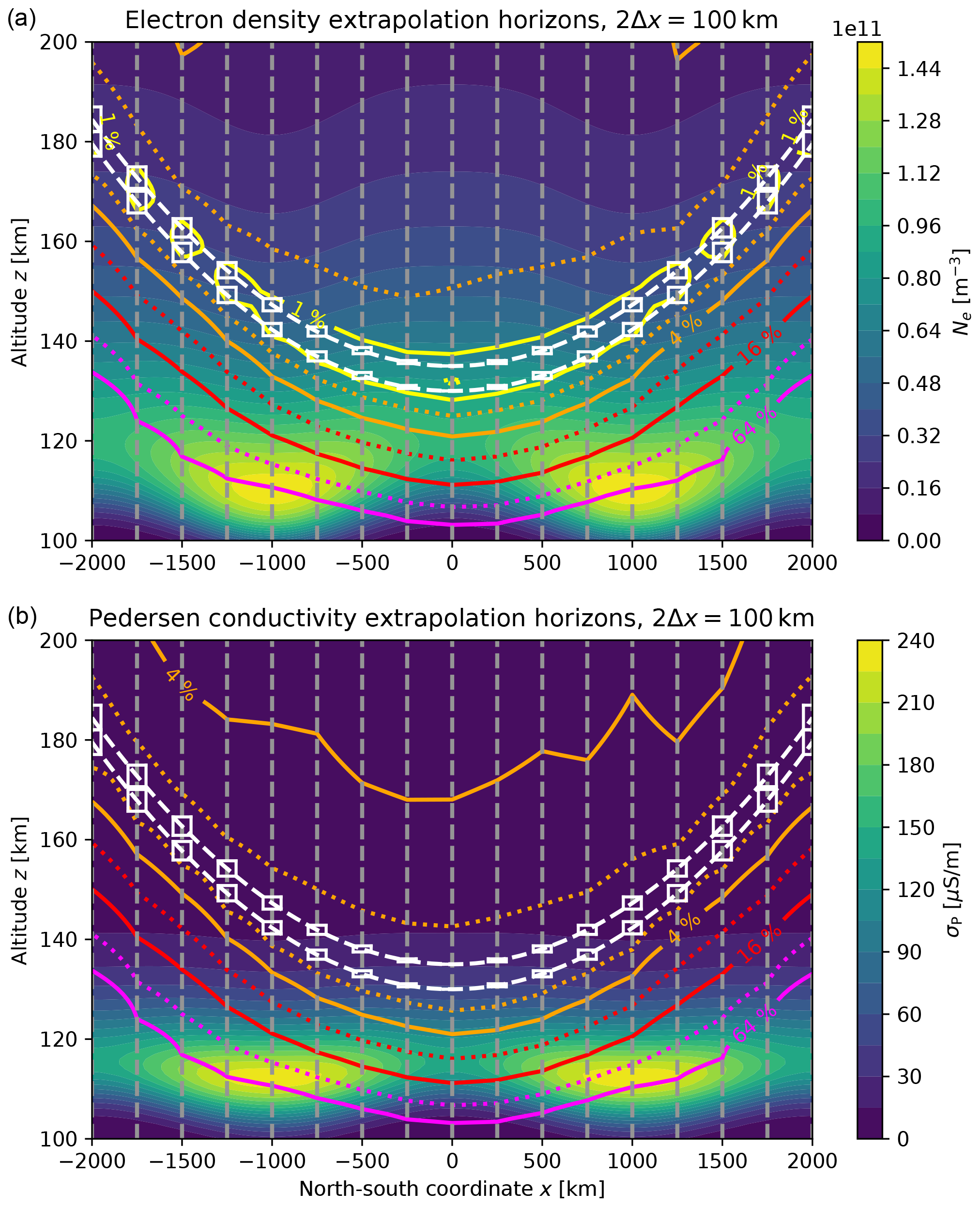
The DIPCont procedure to assess the quality of in situ measurement downward continuation is detailed in Sect. 3. In brief, after choosing an LTI model, representative ensembles of altitude profiles are generated by means of Monte Carlo simulations. The altitude profile ensembles give rise to statistical measures of relative deviation, which in turn allow for estimation of extrapolation horizons, effectively capturing the altitude range where deviations remain within given error thresholds. The basic ideas are illustrated in Fig. 1, displaying electron density and Pedersen conductivity extrapolation horizons for a range of relative error thresholds along the orbits of a dual-satellite mission. Horizontal distance corresponds to the latitudinal (north–south) direction, with the origin of the horizontal axis centered at the highest latitude along the satellite orbits. In the LTI model runs leading to Fig. 1, latitudinal inhomogeneity parameters are set to reproduce the two electron density maxima observed by a polar-orbiting satellite when crossing the auroral oval. See Sect. 4 and Appendix D for details. It is important to note that the filled contour representations of electron density and Pedersen conductivity model distributions mainly serve to provide contextual information, while the essential results of the DIPCont modeling procedure are the extrapolation horizons represented as plain contour lines, in response to the satellite orbit configuration (white lines). The extrapolation horizons of the model run shown in Fig. 1 suggest that for a dual-satellite mission as anticipated in the Daedalus Report for Assessment (ESA, 2020), downward continuation yields relative errors in the range of about 10–50 % at altitudes where electron density and Pedersen conductivity maximize. Implications are discussed in more detail further below in Sect. 4 and contrasted with the single-satellite case.
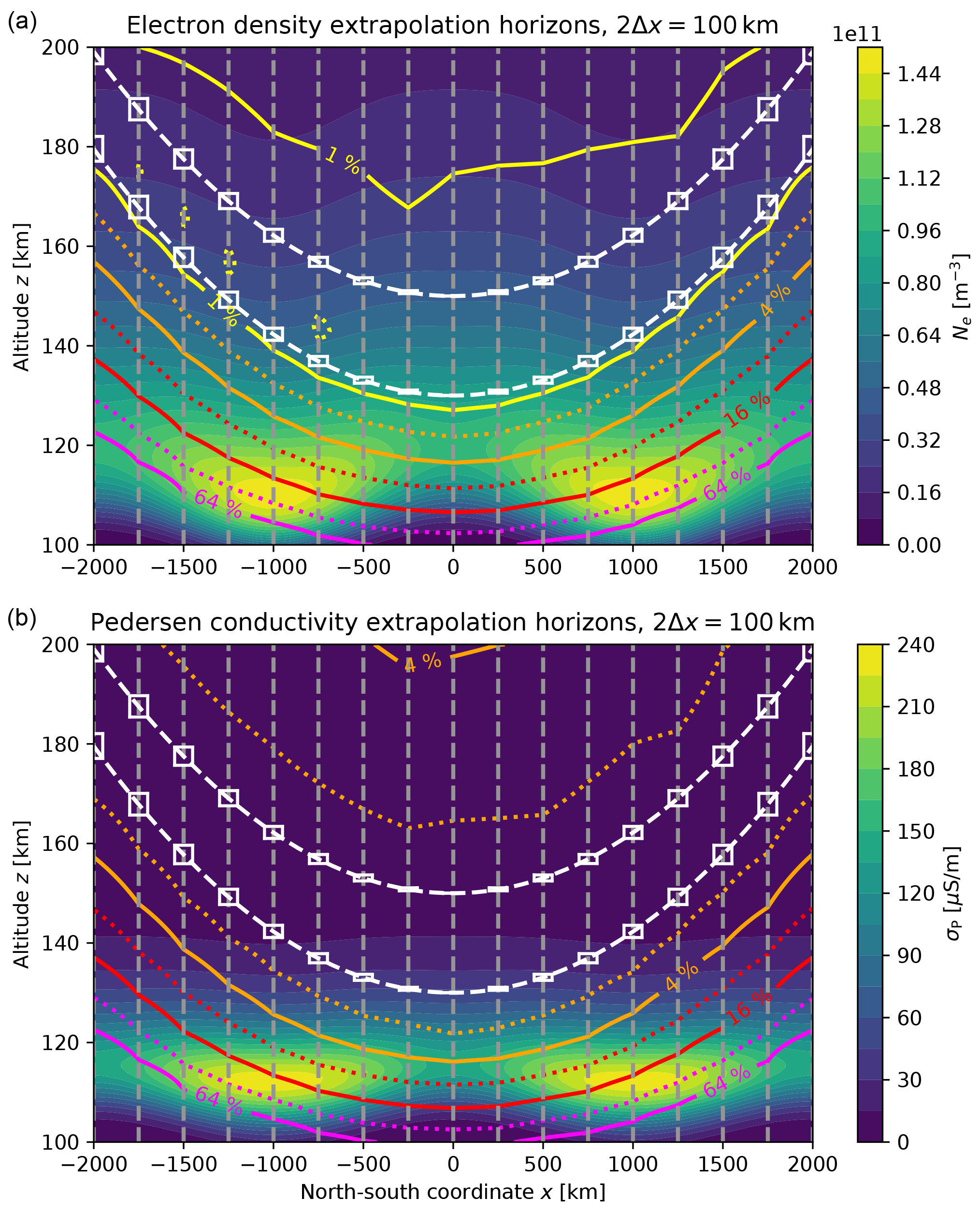
Figure 1Extrapolation horizons and orbit configuration displayed on top of a two-dimensional section of the modeled LTI. (a) Electron density Ne. (b) Pedersen conductivity σP. Horizontal distance corresponds to the latitudinal (north–south) direction, with the origin of the horizontal axis centered at the highest latitude along the satellite orbits. In the LTI model runs leading to this figure, latitudinal inhomogeneity parameters are set to reproduce the two electron density maxima observed by a polar-orbiting satellite when crossing the auroral oval. Synthetic measurements are produced along the two satellite orbits (dashed white lines). The parameters of vertical profiles are estimated using measurements within a window (solid white rectangle) 2Δx in width around the nodes of a horizontal grid (dashed gray lines). Extrapolation horizons (solid and dotted colored lines) for a set of relative error levels are displayed as contours of a relative deviation measure, here the root-mean-square deviation of the ensemble of extrapolated profiles from the synthetic model prediction.
The LTI model used to introduce and demonstrate the DIPCont methodology in this paper is presented in Sect. 2. The parametric model captures the whole LTI temperature range and thus addresses a main source of variability. To limit the number of model parameters and thus also instabilities during model inversion in this initial DIPCont study, LTI variables showing less pronounced changes and ionization source mechanisms are treated in a simplified manner. Furthermore, since the quality of downward continuation is the focus of our study, the LTI model is restricted to E-region physics, with the influence of the F region left for future work.
Further first results are presented in Sect. 4, including a brief comparison between the single-spacecraft and the dual-spacecraft scenario. In Sect. 5, our findings are discussed in the context of important technical parameters and constraints relevant for a low-altitude mission. The body of the paper is concluded in Sect. 6 with prospects for upcoming work. Model derivations and technical details are presented in the Appendices, with particular emphasis on the incorporation of a non-isothermal temperature profile varying linearly with altitude.
Probabilistic measures of extrapolation quality produced by the DIPCont procedure detailed in Sect. 3 are based on synthetic in situ observations predicted by a model of the LTI. As emphasized in space physics textbooks and reviews of the LTI (e.g., Pfaff, 2012; Richmond, 1995), the full complexity of LTI variability and dynamics calls for a full multi-species description, taking into account source and loss processes varying in importance and efficiency as functions of magnetic latitude and local time and further factors. In the future, DIPCont functionality is planned to be included in the Daedalus MASE (Mission Assessment through Simulation Exercise) toolset (Sarris et al., 2023b), designed with the purpose to assess and demonstrate the closure of the mission objectives of the proposed Daedalus mission.
The more complex the LTI model of choice, however, the larger the number of parameters that are to be estimated with a downward continuation of in situ satellite measurements, which in turn tend to negatively affect the stability of model inversion. With these implications in mind, the initial version of the DIPCont package contains a simplified LTI description based on a limited set of parameters. Extrapolation quality of a single but important process, namely the formation of Pedersen conductivity σP, is supposed to be studied in a self-consistent manner. To this end, only a single particle species is considered, and classical photoionization physics is applied to parametrize ionospheric layer formation. Furthermore, as explained in reviews of ionospheric physics (e.g., Rishbeth, 1997), contributions from electron–neutral collisions to the Pedersen conductivity σP peak in the D region but are unimportant at higher altitudes; see also Fig. 4 in Sarris et al. (2023b). We thus arrive at the expression
(e: elementary charge; mi: ion particle mass; Ωi: ion gyrofrequency), suggesting that the altitude variabilities in electron number density Ne and ion–neutral collision frequency νin need to be modeled carefully. Less critical is the dependence of ion gyrofrequency Ωi on magnetic field strength as it does not vary much over the LTI altitude range and is captured with sufficient accuracy by well-established empirical models. Different parametrizations exist for the ion–neutral collision frequency νin (e.g., Palmroth et al., 2021; Huba, 2019; Evans et al., 1977). In general the expressions are directly proportional to the number density Nn of neutral particles. As presented in Appendices A and B, also the self-consistent construction of electron density Ne rests prominently on the Nn profile, which in turn is conveniently modeled in terms of the density scale height . This aspect is chosen as a starting point below in Sect. 2.1 to further explain and motivate the LTI modeling approach.
The LTI model can be summarized in the form , with a vector m of LTI observables and derived functions and a vector p=p(x) of model parameters, separating the primary (strong) dependence on altitude z from the secondary (weak) dependence on horizontal location x in a numerically efficient manner. Note the model functions are local representations of altitude profiles in the sense that they refer to a flexible reference altitude, z0, that can be adapted to the locations where measurements are taken. In the DIPCont development phase it was observed that parameters of model functions in local representations typically showed weaker correlations and could be estimated more reliably, in particular as compared to the regional representations, relying on parameters at some fixed altitude, like the peak electron density height.
As in the Daedalus Report for Assessment (ESA, 2020), the vertical boundaries of the LTI region are assumed to be at zB=100 km (base or bottom-side altitude) and zT=200 km (topside altitude).
2.1 Scale height parameters
As demonstrated in Appendix A, profiles of (neutral gas) pressure Pn and neutral (number) density Nn are conveniently constructed using
where and denote the pressure scale height and the density scale height, respectively. Furthermore, it is shown that
if the pressure scale height
(k: Boltzmann constant; Tn: neutral temperature; g: gravitational acceleration; Rgas: universal gas constant; mn: average particle mass; Mn: average molar mass) changes only with temperature Tn. Equations (4) and (5) further imply that, if temperature Tn varies linearly with altitude z, then and do too. In Appendix A it is shown that the constant inverse gradients
and
are related through
Variations in gravity g across the LTI are in the range of a few percent and can be neglected in this context. Profiles of Tn, Mn, and as predicted by the empirical atmospheric model NRLMSIS 2.0 (Emmert et al., 2021) for different seasons and latitudes are displayed in Fig. S1a–d as part of the Supplement to this paper, indicating that relative variations in average molar mass are indeed significantly smaller than those of neutral temperature. We thus disregard altitude changes in average molar mass Mn as imposed by changes in atmospheric composition and further assume that temperature Tn, pressure scale height , and density vary linearly with altitude in a self-consistent manner as described by Eqs. (4) and (5). According to Eq. (A11), the local density scale height can be obtained using the inverse scale height gradients and the local pressure scale height from the expression
where the subscript 0 indicates that the respective variable is taken at the reference (measurement) altitude z0.
Since in the construction of neutral-density and electron density profiles (Appendix A and B) the scale height parameters are of central importance, their relative change is reflected in the following reference values: at zB, TnB∼200 K, and . Figure S1a–d suggest that the pressure scale height varies by a factor of ∼ 5 across the LTI; thus , and TnT∼1000 K at zT= 200 km. We obtain , γ∼4, , and for the density scale height at the base of the LTI.
2.2 Neutral temperature
Neutral temperature Tn is assumed to vary linearly with altitude z:
The parameters Tn0 and Ln0 are the neutral temperature and the gradient length scale, respectively, at a reference altitude z0. The constant temperature gradient is given by
Using Eq. (A13), the neutral-temperature profile can be expressed by means of the parameters η and as follows:
2.3 Neutral density
The altitude dependence of neutral density Nn for linear scale height profiles is derived in Appendix A, resulting in the following local representation:
see also Eq. (A15). The parameter Nn0=Nn(z0) is the local neutral density, i.e., its value at the reference altitude z0.
2.4 Electron density
The altitude dependence of electron density Ne for linear scale height profiles is derived in Appendix B, resulting in the following local representation:
with ; see Eq. (B16). The parameter Ne0=Ne(z0) gives electron density at the chosen reference altitude z0. Note that Lr0 and χ, the angle of incident radiation with the atmospheric layer normal direction, cannot be estimated separately but only combined as Lr0cos χ. The parameters and η can be inherited from estimations using neutral-temperature and/or neutral-density data, effectively reducing the number of electron density parameters and thus stabilizing the estimation procedure.
The non-isothermal electron density model can also be expressed in terms of the ionization peak parameters, namely the altitude z* and the electron density value :
with and denoting the density scale height at . See Appendix B2 for details. Electron density profiles for identical peak parameters but different values of η are displayed in Fig. 2.
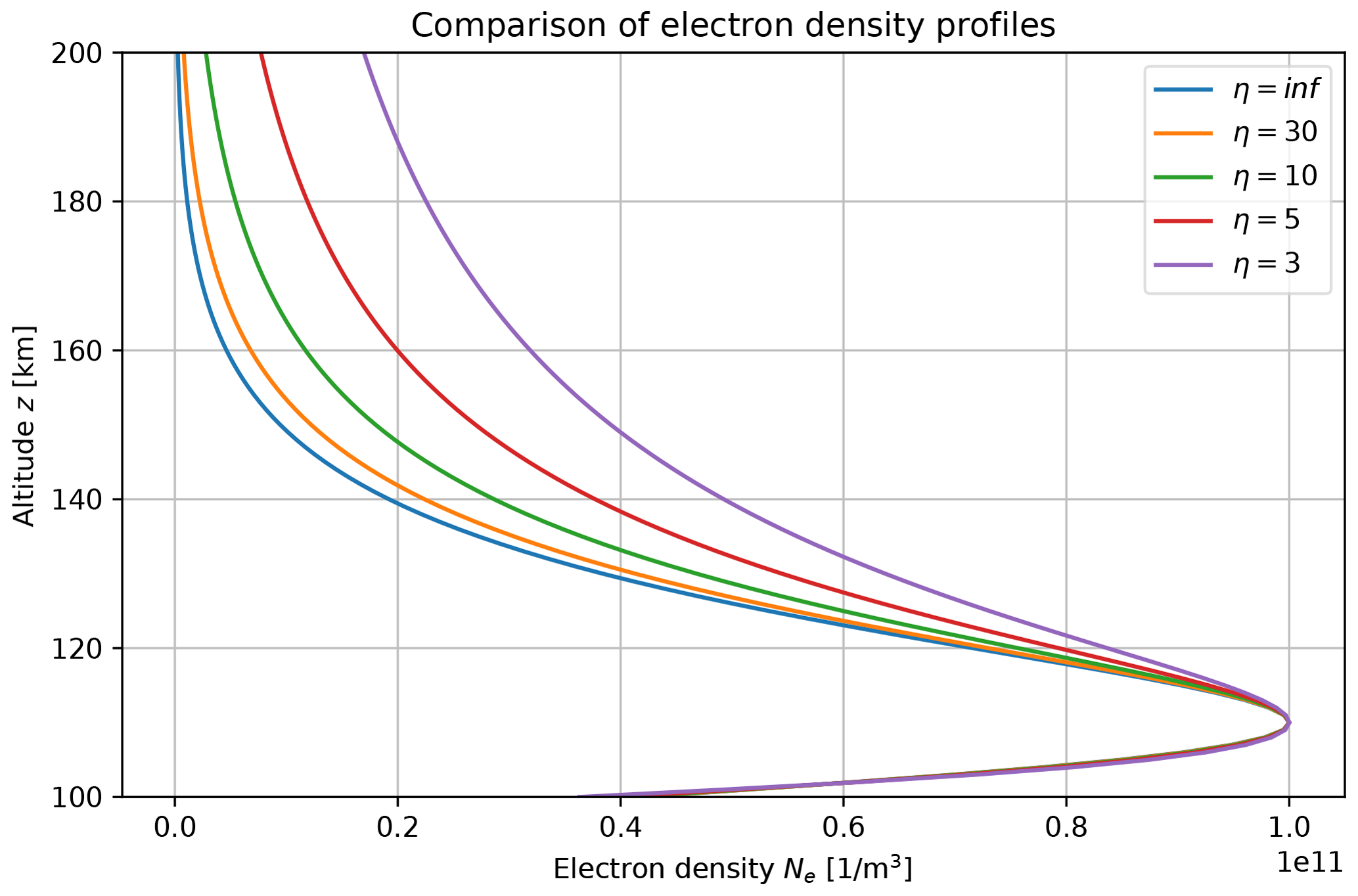
Figure 2Altitude dependence of the non-isothermal electron density model for different values of the inverse neutral-density scale height gradient η. Common electron density peak parameters are , , and . The case η→∞ (in the legend, η=inf) corresponds to the isothermal limit.
The electron density model is designed to describe the ionospheric E layer, assuming that contributions from the F layer are modeled separately and subtracted from the measurements. To account for residuals that may remain after subtraction, the DIPCont package contains a parameter NeF.
2.5 Ion temperature
Temperature profiles obtained by the International Reference Ionosphere (IRI) 2.0 model (Bilitza et al., 2022) indicate that ion and neutral temperatures are very similar throughout the LTI; see Fig. S2a–d. In analogy with the neutral-temperature case, ion temperature Ti is assumed to vary linearly with altitude z:
The parameters Ti0 and Li0 are the ion temperature and the gradient length scale, respectively, at the chosen reference altitude z0.
2.6 Ion–neutral collision frequency
In quantitative terms, collision processes in the partially ionized LTI medium remain inadequately described and are major sources of uncertainties in empirical models (e.g., Palmroth et al., 2021; Heelis and Maute, 2020; Sarris, 2019). At this stage, the DIPCont project is less concerned with optimizing the quantitative description of the LTI, but rather with the quality of parameter estimation extrapolation. While the choice of the best LTI model is certainly important for recovering the real values of targeted observables, further work will be needed by parametric studies, comparison with previous work, and data analysis when a low-perigee mission such as Daedalus (Sarris et al., 2020) provides in situ measurements in the LTI. For our goal here, the chosen variant among the models for ion–neutral collision frequency νin should not matter too much as long as the underlying variability associated with erroneous measurements is captured. To this end, we follow the description of Huba (2019) and write
with the collision cross-section . An even simpler expression could neglect the variation with ion temperature Ti so that νin becomes directly proportional to the neutral density Nn.
2.7 Pedersen conductivity
Using the approximations explained at the beginning of Sect. 2, Pedersen conductivity is given by
for a quasi-neutral two-component plasma when the contribution from electron–neutral collisions is neglected; see also Eq. (1), reproduced here for convenience. Compared to other variables and parameters of the LTI models presented here, the dependence of ion gyrofrequency (qi: ion charge; mi: ion mass) on magnetic field strength B can be determined from measurements or models of the magnetic field with very good accuracy; hence the associated variability should not much affect our results. Furthermore, in the logic of the LTI model constructed for the initial version of the DIPCont package, changes in atmospheric composition and thus average ion mass are disregarded. Inspection of Fig. S2a–d indicates that in the lower part of the LTI (altitudes below about 150 km), being the focus of downward continuation quality in the current study, variations in average ion mass with altitude are relatively small. Hence, altitude variations in ion gyrofrequency are neglected. In the same way as for other LTI model variables, namely through the dependence of the parameters in the vector p=p(x) (see Sect. 2.8 below) on the coordinate x, horizontal variations in magnetic field strength B and thus ion gyrofrequency Ωi can be modeled and are planned to be considered in future work.
2.8 LTI model in compact form
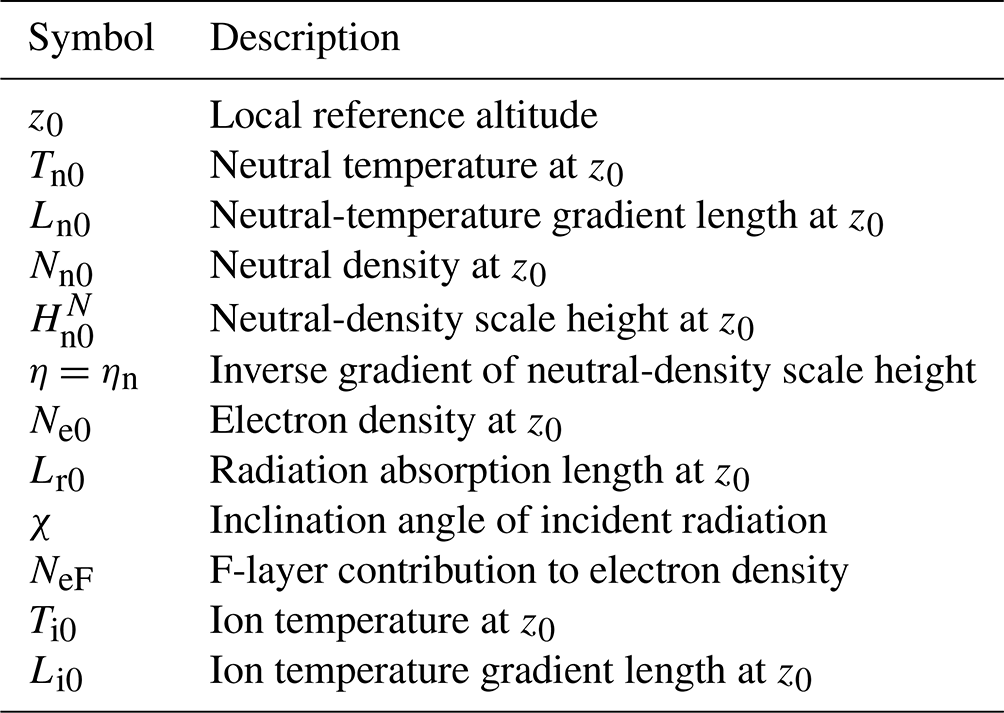
Parameters of model functions in local representation are listed in Table 1.
The description of the DIPCont modeling procedure in Sect. 3 benefits from summarizing the LTI model in compact form as , with parameters , etc. entering the vector p. The parametric functions Tn(z), Nn(z), Ne(z), Ti(z), , and constitute the components of the vectorial function m.
The DIPCont modeling procedure is as follows.
-
Synthetic noise-free measurements are created along anticipated Daedalus satellite orbit sections around perigee at altitudes zj=z(tj) and horizontal distances xj=x(tj). The chosen model parameters are defined by vectors p=p(x#) on a grid of horizontal distances x#. The integration and approximation methods employed for constructing the satellite orbits are described in Sect. 3.1 and in Appendix C.
-
Using the multiplicative noise model presented in Sect. 3.2, synthetic measurements are contaminated by random errors in accordance with relative uncertainties specified in the Daedalus Report for Assessment (ESA, 2020), yielding ensembles of noisy synthetic data sets.
-
For a point x# on the horizontal grid, synthetic data with horizontal distances xj in are considered to produce a least squares estimate of the parameter vector p(x#). Repeating the estimation procedure for all members k of the ensemble of synthetic data sets yields ensembles of model parameters for all horizontal grid points x#. Specifics of the estimation procedure are discussed in Sect. 3.3.
-
With parameter vectors , the parametric model function can be evaluated to obtain ensembles , representing altitude profiles of LTI observables and derived variables such as νin and σP over the entire range of LTI altitudes and for all horizontal grid points x#. The resulting altitude profiles form a representative ensemble in the sense that their statistics are compatible with the model functions and the set of given relative errors. Relative deviation measures of observables and derived variables as functions of altitude are constructed. Finally, the concept of extrapolation horizons, introduced in Sect. 3.4, captures the altitude range where errors are tolerable according to predefined thresholds.
Table 1Parameters of model functions in local representation. The list is partially redundant, e.g., . The parameters Lr0 and χ cannot be estimated independently but only in combination (Lr0cos χ). Boundary data (neutral and ion temperatures at the base of the LTI) are used to constrain the parameters Ln0, η, , and Li0; see Sect. 3.3.
3.1 Satellite orbits around perigee
The DIPCont model offers two options for computing altitudes and horizontal distances along the orbits of satellites around perigee, namely numerical integration by means of the Störmer–Verlet method (e.g., Hairer et al., 2003) and the polynomial approximation
with the acceleration aper at perigee given by
see Appendix C. Here RE is the Earth's radius; ME is the Earth's mass; G is the gravitational constant; zper, Rper, and Vper are the altitude, geocentric distance, and satellite velocity at perigee; is the Earth's gravitational acceleration at geocentric distance Rper; Rapo is the geocentric distance at apogee; and is the orbital eccentricity. For the parameter range considered in this study, the deviation of the polynomial approximation from the more precise orbit integration is on the order of a few hundred meters; see Fig. S4b of this report.
The observation time Tobs spent by Daedalus in the LTI during a perigee pass controls the amount of data that can be gathered for statistical investigations. Using the quadratic orbital approximation around perigee, Tobs is twice the time needed to move from z=zper to the upper boundary at z=zT; thus , , and
The variations in Tobs with apogee altitude in the range of for the three perigee altitudes zper=115, 130, and 150 km are displayed in Fig. 3. Raising the perigee from 115 to 130 km yields a small reduction in observation time by about 10 %. Within the range of orbital parameters considered here, the overall amount of data gathered during a perigee pass turns out to depend only moderately on apogee altitude zapo, with a relative difference of not more than about 20 % for changes in zapo between 2000 and 3000 km.
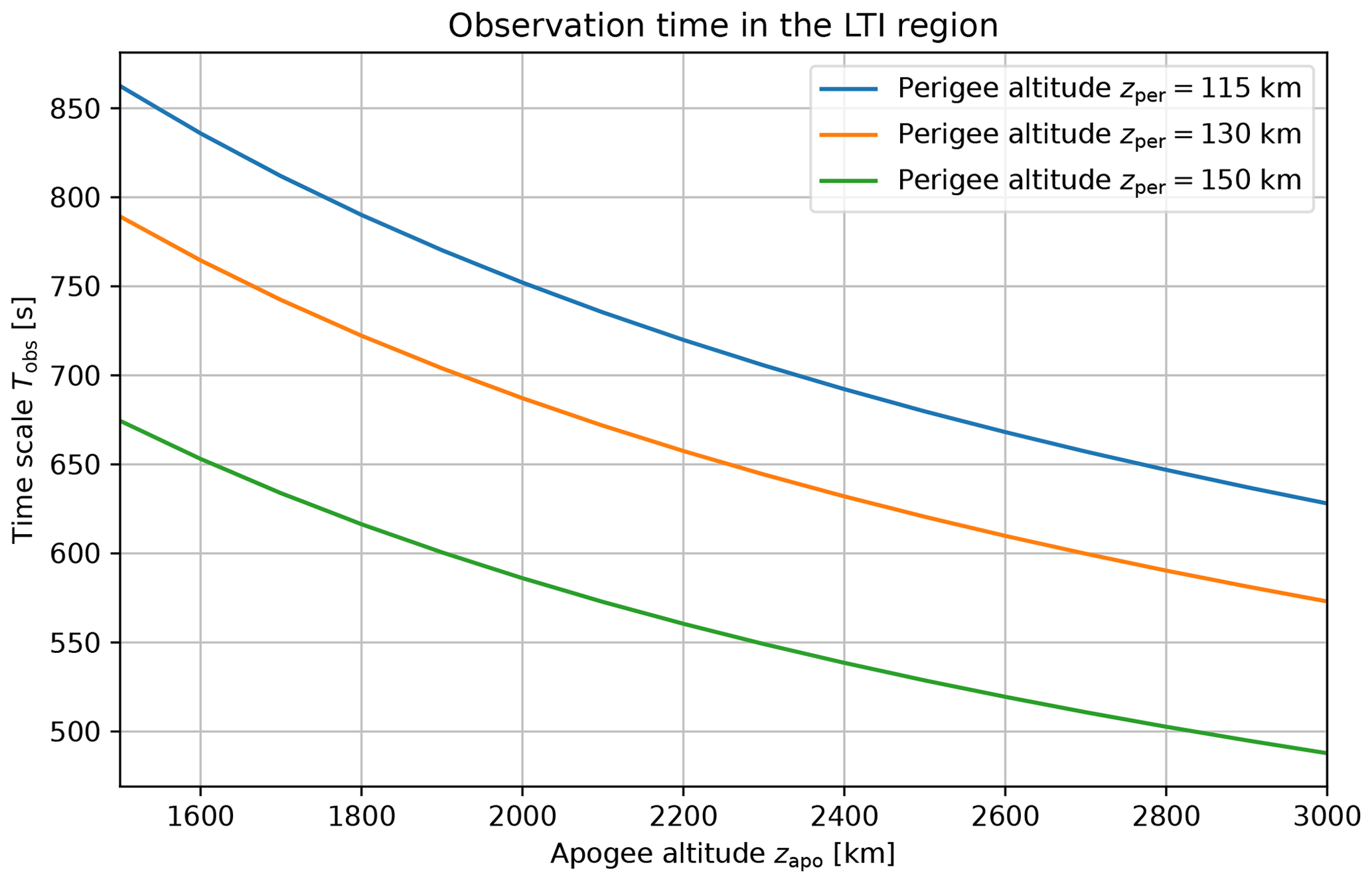
Figure 3Observation time Tobs in the LTI versus apogee altitude zapo for three different values of perigee altitude zper. The topside of the LTI is assumed to be at zT=200 km.
When dual-satellite missions to the LTI are considered, the question arises as to how synchronous the measurements are with respect to ground horizontal distance x, assuming the two spacecraft share the same orbital plane, have identical semi-major axes and thus orbital periods, and pass through their perigees at the same time. Figure S4a illustrates how visit times of ground horizontal distances are expected to differ for two satellites with perigee altitudes of 130 and 150 km. Differences in satellite visit times turn out to be on the order of seconds.
3.2 Synthetic measurements and positivity constraints
Synthetic measurements of an observable at altitudes are constructed from a parametric model function producing predictions that are contaminated by random errors from a suitable probability distribution. The model parameter vector p is estimated through minimization of a cost function. Following the standard least squares approach, the cost function is chosen to be the error-scaled square deviation
The observables of interest Tn, Nn, Ne, and Ti are all positive; hence a straightforward additive noise model would not be appropriate as it may produce negative synthetic data. Furthermore, instrumental uncertainties as provided in the Daedalus Report for Assessment (ESA, 2020) are typically specified as relative (multiplicative) errors. Both issues are addressed by considering as model predictions and data not the positive observables as such but their (natural) logarithms and relative uncertainties for the random errors . In the case of a (neutral or electron) density N, one obtains
where represents Gaussian noise (normally distributed random numbers with zero mean and unit variance), and N=N(z) refers to the (positive) density model. Then
so that positivity is guaranteed. Furthermore,
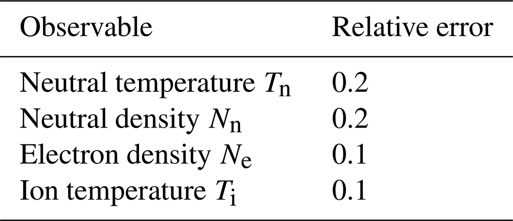
showing that the parameters σj correspond to relative error levels. Table 2 summarizes the values used in this report.
Table 2Relative error levels used in this study, according to Table 2 of the Daedalus Report for Assessment (ESA, 2020).
In general, the parameters enter the logarithms of model functions nonlinearly, and an iterative estimation procedure is required.
3.3 Parameter estimation strategies
The model parameters listed in Table 1 are estimated from observations of neutral temperature Tn, neutral density Nn, electron density Ne, and ion temperature Ti as follows.
-
For a given horizontal grid location x#, data within the interval are considered. The effective window width is 2Δx; see the solid white rectangles in Figs. 1 and 4.
-
From Tn data and constraining the neutral-temperature profile at the LTI lower boundary zB as explained below, infer Tn0, , and η. See Eq. (10) and Sect. 2.1.
-
Using and η, estimate Nn0 from Nn data. See Eq. (13).
-
Using and η, estimate Ne0 and Lr0cos χ from Ne data. See Eq. (14).
-
From Ti data and a suitable constraint at the lower LTI boundary zB in analogy to the neutral-temperature case, infer Ti0 and Li0. See Eq. (16).
Altitude profiles of these observables allow for construction of the height dependence of derived variables such as ion–neutral collision frequency νin and the Pedersen conductivity σP; see Eqs. (17) and (18), respectively.
3.3.1 Lower LTI boundary constraints
As explained in Appendix A, Eqs. (A10) and (A13), the linear density scale height profile can be parametrized using and η in the form
It is important to note that the profile takes center stage in the LTI models of the observables Tn, Nn, and Ne. While the local temperature amplitude Tn0 is essentially an average of local temperature data around an altitude z0, and the same applies to the local pressure scale height obtained from Tn0 by simple multiplication, the inverse density scale height gradient η and thus also the local density scale height parameter are very challenging to estimate from purely local data with little variance in altitude, as suggested already by the standard error of the slope in linear regression analysis. Fortunately, neutral temperature at the base of the LTI is known with reasonable tolerances from atmospheric models (e.g., Picone et al., 2002; Emmert et al., 2021). This remote data point constitutes a valuable constraint for estimating the density scale height profile. To incorporate model uncertainties and expected deviations from actual values, boundary data at the base of the LTI are contaminated by random errors according to the approach described in Sect. 3.2.
To be specific, the pressure scale height gradient, constant under the assumptions discussed in Sect. 2.1 and Appendix A, can be obtained from its values and at z0 and the LTI base altitude zB, respectively, as follows:
The inverse gradients γ and η of pressure scale height and density scale height, respectively, are related by Eq. (8) through ; thus the parameter η is given by
where TnB denotes the neutral temperature at zB. The local density scale height can now be obtained from Eq. (9) as
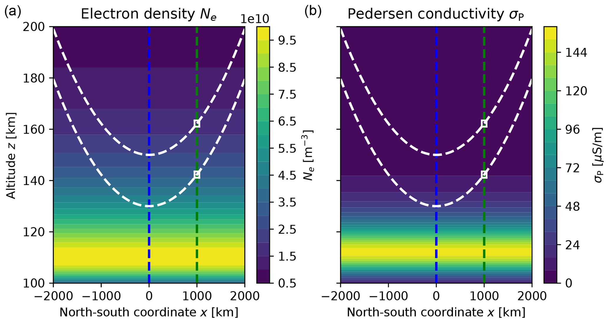
Figure 4Model distributions of electron density Ne (a) and Pedersen conductivity σP (b) in the LTI. Synthetic measurements are produced along the two satellite orbits (dashed white lines). The parameters of vertical profiles are estimated using measurements within a window (solid white rectangle) around two locations in the horizontal direction (dashed blue and green lines).
3.3.2 Linear estimation of electron density parameters
The logarithm of the electron density model considered here,
can be combined with the logarithm of the neutral-density model,
to find
showing that and can be obtained from linear regression of versus with . Since the parameters η and are available as estimates from Tn modeling, and Nn0 is known from Nn modeling, Ne0 and Lr0cos χ can be computed from the linear coefficients a and b; hence this special case does not necessitate an iterative parameter estimation approach.
3.4 Error profiles and extrapolation horizons
With being a single set (k=1) of synthetic measurements and j∈[#] indicating that horizontal distances are selected to be within ±Δx around a predefined grid point x#, the estimation procedure yields a specific estimate of the parameter vector p(x#). In a Monte Carlo setup, different instances of random errors are applied to the model predictions to produce data sets . The ensemble of data sets gives rise to an ensemble of parameter vectors , which in turn, when entered in , yields an ensemble of profiles for the entire range of altitudes z and at each point x# of the horizontal coordinate grid.
The procedure is illustrated in Figs. 4 and 5. Figure 4 shows the model functions and the satellite orbits used for computing the predictions that enter the Monte Carlo simulation. The ensemble of altitude profiles generated from the Monte Carlo distributions of model parameters is visualized in Fig. 5 by means of selected quantiles evaluated at the vertical grid of LTI altitudes.
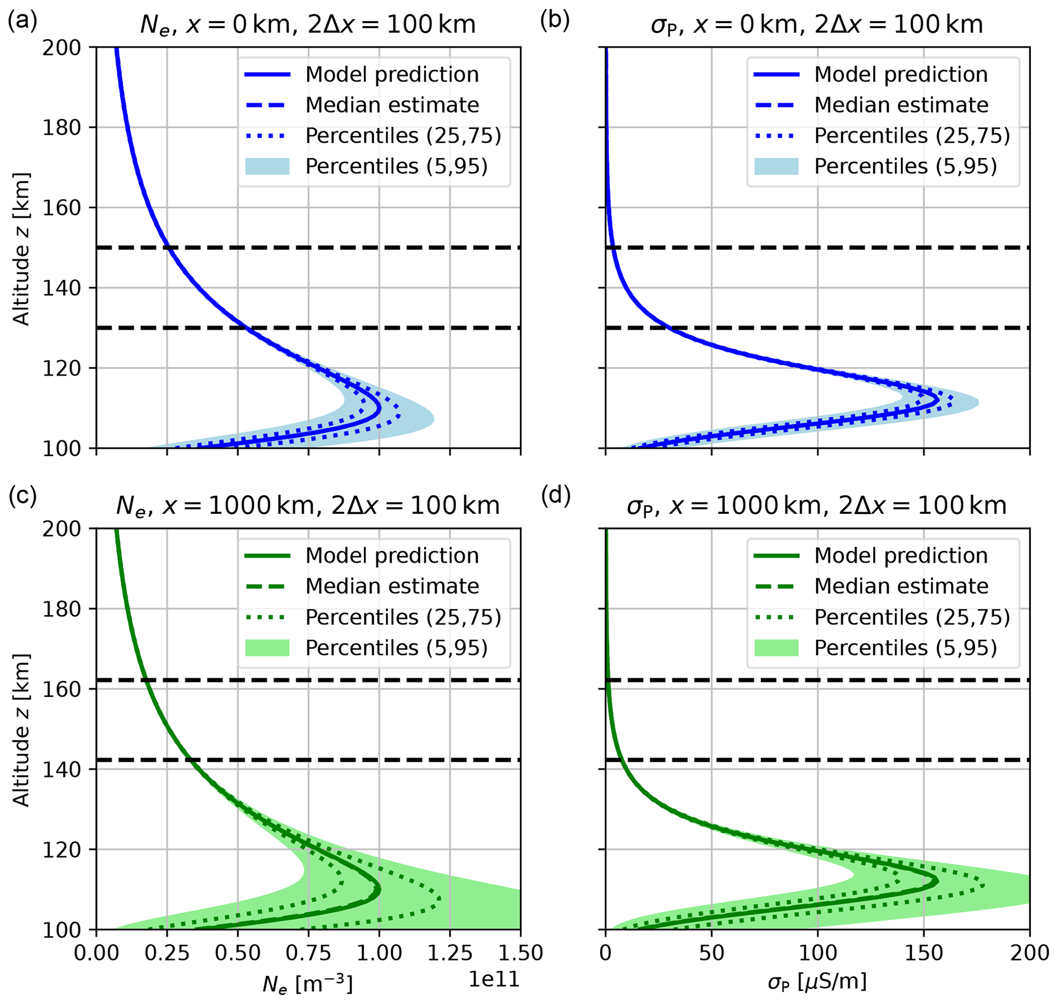
Figure 5Visualization of the ensemble of altitude profiles generated from the Monte Carlo distributions of model parameters. Shown are selected quantiles evaluated at the vertical grid of LTI altitudes. (a, c) Electron density Ne. (b, d) Pedersen conductivity σP. (a, b) Center position (dashed blue line) in Fig. 4. (c, d) Right position (dashed green line) in Fig. 4.
The ensemble of altitude profiles forms the basis for quantifying extrapolation quality through measures of relative deviation from a model prediction. Suppressing altitude and horizontal grid dependencies and considering only a single model variable μ with ensemble members , the root-mean-square deviation is given by
Figure 6 shows the altitude profiles of relative root-mean-square deviation for the variables and horizontal locations as in Figs. 4 and 5.
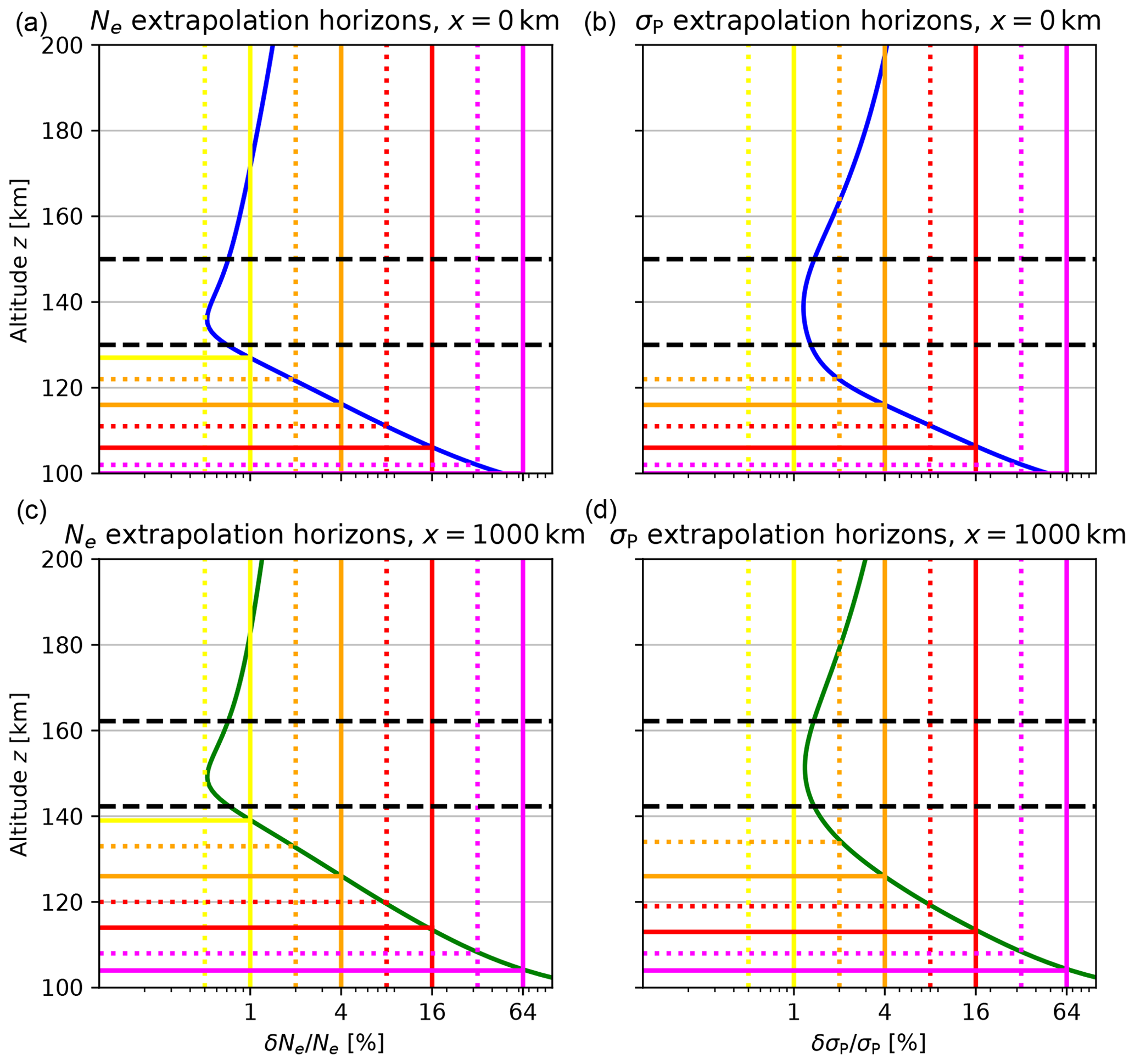
Figure 6Solid lines (blue and green) give the relative root-mean-square deviations of Monte Carlo altitude profiles from the respective input model profiles at two horizontal locations. Vertical dotted and solid lines represent a set of chosen error levels, ranging from 0.5 % and 1 % (yellow) to 32 % and 64 % (magenta). The corresponding horizontal lines show the extrapolation horizons indicating at which altitude the relative deviation equals the respective error level. (a, c,) Electron density Ne. (b, d) Pedersen conductivity σP. (a, b) Center position (dashed blue line) in Fig. 4. (c, d) Right position (dashed green line) in Fig. 4.
Figure S3 provides additional information on this DIPCont model run; visualizing model distributions; ensembles of altitude profiles; and extrapolation horizons also for neutral temperature Tn, neutral density Nn, ion temperature Ti, and ion–neutral collision frequency νin.
Alternative relative deviation measures considered in the DIPCont package are based on the empirical distribution of absolute deviations , e.g., the average absolute deviation from the model prediction μ,
or selected quantiles of the distribution.
3.5 Implementation
The DIPCont model is implemented as a bundle of Python instructions and functions collected in three modules.
In the module DIPContBas.py, the basic setup of the DIPCont framework is defined, e.g., LTI region boundaries and boundary values, satellite orbit parameters, horizontal grid locations, and auxiliary plot parameters. Furthermore, it also provides configurational variables that are exchanged between DIPCont functions and modules, e.g., parameters shared by different parametric models.
The module DIPContMod.py provides parametric model functions of LTI variables and plot routines.
The module DIPContEst.py is concerned with Monte Carlo parameter estimation and profile continuation. Estimation of parameters that enter the model functions nonlinearly is accomplished by the function curve_fit() from the module scipy.optimize, whereas linear parameter estimation is performed using the function linregress from the module scipy.stats. Monte Carlo ensembles of parameters and altitude profiles are stored in pandas DataFrames.
The three DIPCont modules are provided in the Supplement to this report, together with Jupyter notebooks to explain and illustrate their usage.
The major ingredients of the DIPCont processing chain, namely generation of synthetic in situ measurements along satellite orbits, Monte Carlo simulations of vertical profiles, and construction of extrapolation horizons, are summarized in Figs. 4–6, displaying electron density Ne and Pedersen conductivity σP as two variables of key importance for the structure and the dynamics of the LTI. As indicated by Eq. (1) and the respective profiles in Fig. 5, electron density makes the main contribution to the peaked height variation in Pedersen conductivity, with secondary contributions of neutral density and possibly ion temperature through the parametric form chosen for the ion–neutral collision frequency; see Sect. 2.6 and also Fig. S3. Furthermore, Pedersen conductivity controls the height variation in Joule heating, whose characterization is one of the main scientific targets of the proposed Daedalus mission (ESA, 2020). In the neutral wind reference frame, Joule heating is , where the subscript ⟂ indicates a vectorial component perpendicular to the ambient magnetic field direction . Height variations in E⟂ are negligible according to the following rationale; see, e.g., Rishbeth (1997). Due to high parallel conductivity, the electric field component parallel to vanishes, i.e., , where s is the magnetic field line coordinate, and Φ denotes the electric potential. The electric field component Eq in a direction perpendicular to captured by a coordinate q then satisfies .
When instead of two selected horizontal locations as in Fig. 6 an equidistant grid of horizontal coordinates is defined for DIPCont simulations and the construction of extrapolation horizons, the results can be displayed together with the underlying model distributions and satellite orbits as in Fig. 1. In the following examples, such displays are used to visualize DIPCont results for different spacecraft configurations. Section 4.1 offers a first qualitative assessment of extrapolation quality in terms of varying inter-spacecraft distance. Section 4.2 contrasts the performance of the dual-spacecraft configuration considered so far with the results of the single-spacecraft case.
Note that the horizontal axis corresponds to the latitudinal (north–south) direction. In the simulations that led to Figs. 4–6, horizontal variations were disregarded for better comparability. In Fig. 1 and in the following, latitudinal inhomogeneity of electron density is meant to reproduce the two maxima observed by a polar-orbiting satellite when crossing the auroral oval. The highest latitude corresponds to the origin of the horizontal axis. Since the physics of energetic particle precipitation is not incorporated in this initial version of the DIPCont package, the horizontal variation in electron density expected for an auroral oval crossing is prescribed through ad hoc choices of horizontal electron density peak parameter profiles; see the option LTIModelType='NeAuroralZoneCrossing' in the DIPCont code as part of the Supplement to this report. The functional forms of horizontal electron density peak parameters are given in Appendix D.
4.1 Varying inter-spacecraft distance
Extrapolation of two-point measurements is expected to perform best if the spatial separation matches the relevant physical length scale. In the LTI this should be the (local) density scale height, in the range of 10–20 km for altitudes above 130 km, as in our example of a dual-spacecraft setup with perigee altitudes of 130 and 150 km; see Fig. 1. The inter-spacecraft distance remains close to 20 km throughout the whole orbit section and thus also to the density scale height as the relevant physical scale. Note that in all dual-satellite DIPCont model runs presented in this paper, apogee distances of the second satellite have been adjusted such that the sum of perigee and apogee distances are identical for both satellites and thus also the semi-major axes and the orbital periods.
Figure 7 displays extrapolation horizons for the same simulation setup except that the perigee altitude of the second satellite is reduced to 135 km, producing an inter-spacecraft distance at perigee of only 5 km. The separation is now smaller than the local density scale height with values of about 15 km at altitudes around 150 km. Compared to Fig. 1, the errors are increased and the extrapolation horizons reduced. The changes are not dramatic but enough to show that inter-spacecraft distance is a parameter to be considered when extrapolation quality is supposed to be optimized.
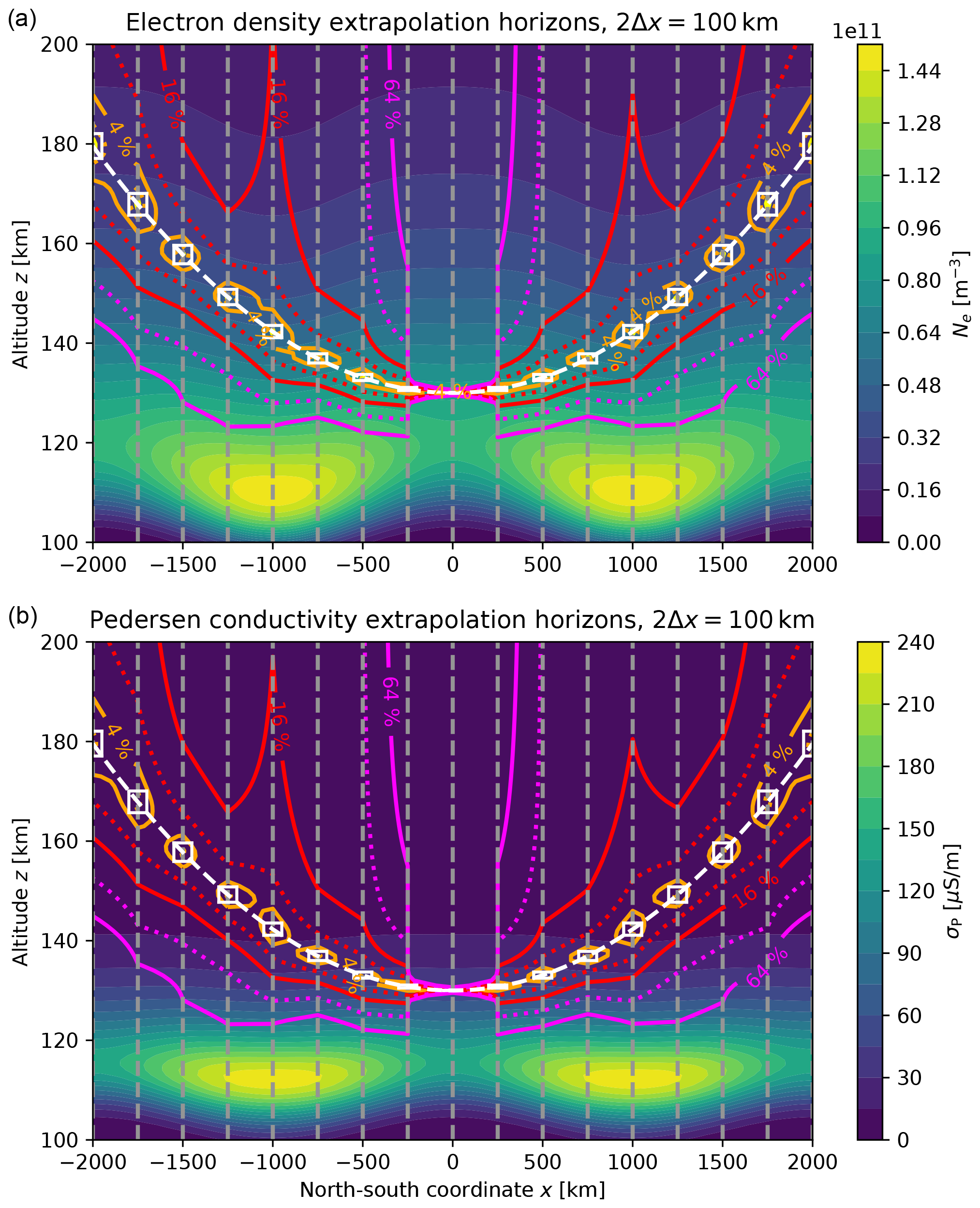
4.2 Single-satellite case
To check how much a second satellite improves extrapolation quality, the Monte Carlo simulations summarized in Fig. 1 are repeated for the single-spacecraft case, with all other parameters left unchanged. The resulting extrapolation horizons are shown in Fig. 8. Compared to ionospheric profile continuation from dual-spacecraft observations, the single-spacecraft case yields significantly worse results, with extrapolation horizons collapsing into the orbit near the perigee due to lacking variability in altitudes. Away from the perigee, the orbital motion of the satellite during the time corresponding to the horizontal window width 2Δx yields some height range that allows for profile reconstruction but with significant errors. The peaks in electron density and Pedersen conductivity are clearly outside the largest considered error level of 64 %, while Fig. 1 shows that in the dual-spacecraft case the peaks are between the 16 % and 32 % error levels.
Our first results suggest that altitude profiles of key LTI variables can be reconstructed with sufficient accuracy from in situ measurements if the effective altitude range covers relevant physical scales such as the local density scale height . This is the case for a dual-spacecraft configuration with an inter-spacecraft separation of 20 km at perigee; see Figs. 1 and 4–6. By two-point sampling, one can retrieve the vertical profiles of electron density and Pedersen conductivity essentially down to the bottom of the LTI region, a few scale heights under the lower satellite and including the peak altitudes. For Pedersen conductivity, errors are expected in the range of about 10–50 %, with the peak altitude and most of the conductivity within the 32 % extrapolation horizon in the chosen example, consistent with rocket observations (Sangalli et al., 2009).
Given the current knowledge of key LTI variables, error levels of about 10–50 % may well improve the situation. An important motivation behind the Daedalus proposal was the large error margin in Joule heating estimates, with a major contribution by errors in conductance (height-integrated conductivity). Thus, Sarris et al. (2020) pointed out that for a substorm event investigated by Palmroth et al. (2005), there were differences of up to 500 % between three proxies for the Joule heating rates integrated over the Northern Hemisphere. Even if this setup cannot be directly compared to our virtual environment, the order-of-magnitude difference between the two error margins looks encouraging for follow-up work on ionospheric profile continuation.
The DIPCont framework allows economical and technical questions regarding the impact of different LTI mission cost factors to be addressed. On the one hand, a dual-spacecraft mission seems to automatically imply higher costs because a second satellite needs to be built. On the other hand, a major cost driver of any deep LTI mission is the necessary amount of propellant that is required in order to maintain a spacecraft in orbit due to enhanced atmospheric drag at very low perigee altitudes. Since in a dual-spacecraft setup the role of the lower perigee satellite can be shared, each of the two probes would have to carry half of the total amount of propellant required to maintain the same total observation time required by a single-satellite mission. Moreover, the necessary amount of thermal shielding depends as well on perigee altitude, and each of the two probes would have to withstand the maximum thermal stress at perigee less often. Our findings show that the two-point setup allows for a more effective extrapolation to lower altitudes, which in turn means that a higher perigee may well be a meaningful option.
Data processing would also benefit from raising the perigee. As shown by simulations carried out for the technical assessment of Daedalus (ESA, 2020), a hydrodynamic shock develops in front of the spacecraft at altitudes under ∼120–130 km, complicating the retrieval of unperturbed data from the observed ones. Another LTI mission parameter considered in this paper is the apogee altitude controlling the proximity to the Van Allen belts and thus the necessary amount of radiation shielding but also affecting the available LTI observation time near perigee. The analysis presented in Sect. 3.1 shows that the amount of data gathered for statistical studies depends only moderately on apogee altitude.
The current version of the DIPCont framework concentrates on the E layer, assuming that contributions from the F layer can be disregarded or subtracted before processing, e.g., using the NeQuick approach to model topside ionospheric sounding data (Pignalberi et al., 2020). The DIPCont package contains a parameter NeF to study the effect of F-layer residuals on extrapolation quality in future work.
The first results presented here are planned to be validated and extended in more extensive studies. Besides varying orbital parameters such as perigee altitude and inter-spacecraft distance, the impact of numerical parameters such as the horizontal selection window, 2Δx, needs further investigation. As already commented in Sect. 2.6, alternative functional forms for modeling ion–neutral collision frequencies or other variables may also be considered.
The DIPCont methodology introduced in this paper is designed to assess the quality of downward continuation of LTI variables using in situ satellite measurements and parametric models. While first results have been obtained with a simplified LTI description based on a single particle species, the Monte Carlo simulation machinery in DIPCont is not constrained to a particular model setup. By quantifying the quality of extrapolated in situ measurements, DIPCont can help to assess the science return of specific configurations and thus to optimize the parameters of upcoming LTI missions.
First DIPCont tests, performed on electron density and Pedersen conductivity, show promising results, to be consolidated by further parametric studies. Application of DIPCont to a modeled event, like the geomagnetic storm event of March 2015 addressed in the Daedalus Report for Assessment (ESA, 2020), is an upcoming target. This could be performed using the capabilities of the Daedalus MASE toolset (Sarris et al., 2023b). Future studies are planned to include Joule heating, which was a major driver of the Daedalus mission proposal. To investigate auroral processes and the electrodynamics of magnetosphere–ionosphere coupling, ionization through energetic particle precipitation needs to be incorporated. The Hall current nature of auroral electrojets calls for including electron–neutral collisional interaction as a major contributor to Hall conductivity formation.
Coordination between an LTI mission, like Daedalus, and a topside mission, like Swarm or DMSP (Defense Meteorological Satellite Program), would enhance the return of both missions. As an example, reconstruction of vertical profiles of ionospheric conductivity based on LTI observations could help to calibrate topside estimates of the conductance, while topside electron density could provide upper continuation and constrain the height-integrated total electron content (TEC) inferred from LTI data. Combination with ground-based observatory data such as ionosondes would offer further valuable constraints to DIPCont and thus enable more comprehensive modeling of the LTI.
Consider an atmospheric layer dominated by possibly several neutral constituents with an average or representative particle mass mn, total pressure Pn, mass density ϱn, effective neutral number density , and temperature Tn. Under hydrostatic conditions, , where z is altitude, and g is gravity (gravitational acceleration), assumed to vary so little within the layer that it can be safely considered constant. Using the ideal gas law Pn = NnkTn, where k denotes the Boltzmann constant, one obtains with the pressure scale height
Rearranging and integrating leads to
where the altitude dependence of directly reflects the change in temperature Tn with z.
Analogous differential and integral expressions for the neutral density, namely and
are derived as follows. Combining the differential of the ideal gas law with the hydrostatic condition yields and thus . Since , one obtains
Therefore, the density scale height in the expression is given by
To be more specific, we suppose the neutral temperature Tn varies linearly with altitude z,
where Tn0 is the temperature at a reference altitude z0, and denotes the local gradient length. Then
with
so that the pressure scale height gradient is constant and thus also the gradient of density scale height:
The linear profile of density scale height is given by
with
Here
denotes the inverse gradient of pressure scale height. The inverse gradient of density scale height
is related to γ through .
In the non-isothermal case Ln0<∞, integrating gives the expression
Hence, the altitude profile of number density (Eq. A3) is given by
In the isothermal limit, η→∞, , and thus , and through Eq. (A11).
Following the approach first presented by Chapman (1931), the ionization rate per unit volume q is expressed in terms of the intensity I of ionizing radiation, the ionization efficiency κ, the angle χ of incident radiation with the atmospheric layer normal vector, the radiation absorption cross-section σr, and the neutral density Nn as . Here z is altitude, and the z axis is pointing upwards as before. The function q=q(z) is also called the production function. Although originally proposed for photoionization, the Chapman approach may also be applied to ionization by precipitation of energetic particles as in the auroral region if model variables and coefficients are properly interpreted.
The intensity I satisfies the differential equation
with the solution
where z∞ and I∞ refer to an upper boundary sufficiently remote from the atmospheric layer.
Using , the production function q can be rewritten as q = κ σrNnI and thus
The ionization peak altitude z* is obtained from the condition
where the prime denotes differentiation with respect to altitude z. Considering Eqs. (A3) and (A14) gives rise to , and , and defining the radiation absorption length Lr=Lr(z) by
the general ionization peak condition is conveniently expressed as
B1 Local representation of electron density
Assuming the neutral temperature Tn varies linearly with altitude z, the altitude dependence of electron density was modeled by Gledhill and Szendrei (1950). Since their formulation does not fit well with the DIPCont nomenclature used in the current report, an independent and extended derivation is presented now. Using and η<∞, the altitude profile of neutral number density can be written in the form
see Appendix A and Eq. (A15). Integration gives
In this LTI modeling context it is safe to assume that the regional temperature increase with altitude is moderate enough to ensure , then η>1. Furthermore, the altitude z∞ is chosen to be large enough for the contribution from the value at to be negligible. We obtain
by using Eq. (A14). Defining
the radiation intensity profile assumes the form
where Lr0=Lr(z0). The neutral density (Eq. A15) is rewritten as
so that the production function (Eq. B3) assumes the form
In the isothermal limit, η→∞, , , and the isothermal Chapman production function (Chapman, 1931) is recovered.
In static equilibrium of photoionization and quadratic recombination, with the recombination coefficient α; thus . Using
we obtain
B2 Representation of electron density in terms of ionization peak parameters
A meaningful regional representation of the electron density can be constructed by means of the ionization peak parameters. For a given incident radiation angle χ, the altitude z* of the electron density maximum can be expressed in local parameters as follows:
where
The electron density peak value is
With z* as the reference altitude, , we can take advantage of the condition (Eq. B6) ; thus
where , and denotes the density scale height at . This representation shows that χ is only an implicit parameter of the electron density model and cannot be inferred from knowledge of the peak parameters.
Consider a Kepler orbit with radial distance r=r(t) and azimuth ϕ=ϕ(t), where t denotes time. Distance and velocity at perigee are Rper and Vper, respectively. The corresponding variables at apogee are Rapo and Vapo, the gravitational constant is G, and the planetary mass is M. Combining the conservation laws for angular momentum,
and total energy E (here normalized by the test mass m),
yields the following expression for the perigee velocity in terms of perigee and apogee distances:
where is the value of Earth's gravitational acceleration at geocentric distance Rper. The radial velocity satisfies
Differentiating this expression and dividing by yields
Evaluation at perigee r=Rper gives
Inserting the expression for yields
where is the orbital eccentricity. The altitude z is related to radial distance r and the Earth's planetary radius RE through . At perigee, t=0, and z=zper. The parameter coincides with the radial acceleration at perigee . Hence, orbital altitudes around perigee are approximately given by the quadratic function
To the same approximation order, the angular momentum conservation condition can be integrated to yield approximate azimuths ϕ=ϕ(t). In insert , then expand
and integrate to obtain
The corresponding horizontal distances at the Earth's surface are then given by . By using Eq. (C9), this can be further processed to yield
The leading term is ground distance for a circular orbit. The correction produced by the second term is proportional to eccentricity.
In the initial version of the DIPCont package, the horizontal variability in electron density profiles is controlled by the keyword argument LTIModelType. Setting LTIModelType='NeAuroralZoneCrossing' produces two electron density maxima along the horizontal (latitudinal) axis as observed by a polar-orbiting satellite when crossing the auroral oval; see Figs. 1, 7, and 8. More specifically, the horizontal (x) variations in peak altitude and peak electron density in Eq. (15) are prescribed by the ad hoc parametrizations
with
so that f=f(x) varies between zero and one. The parameters xL and xR are the horizontal boundaries of the modeling domain, here chosen to be xL= −2000 km and xR= 2000 km. The values of the electron density peak parameters used in the model runs leading to Figs. 1, 7, and 8 are as follows: 110 km, 10 km, , .
All LTI model parameters for the simulation runs of the current report, including the horizontal electron density profile parameters, are provided in the configuration file DIPContBas.py as part of the Supplement.
The DIPCont framework is implemented in three Python modules: DIPContBas.py, DIPContMod.py, and DIPContEst.py. The modules are provided in the Supplement to this report, together with Jupyter notebooks to explain and illustrate their usage. The DIPCont code is planned to be migrated to a public repository.
This study does not make use of external data sets, only sets of synthetic data produced internally by the Monte Carlo simulation code, which are then employed for estimating the variability of ionospheric profiles.
The supplement related to this article is available online at: https://doi.org/10.5194/gi-12-239-2023-supplement.
The DIPCont project emerged from meetings of the SIFACIT project team (OM, AB, JV, NS) with the Daedalus/MASE workgroup at the Democritus University of Thrace (TS, ST, TB, DB, PP). JV developed the DIPCont methodology and the underlying theory, wrote the Python code and the first draft of the manuscript, and coordinated the writing of the paper. OM initiated LTI profile extrapolation under the Daedalus Phase-0 science study, followed on by the activity of the SIFACIT team, and contributed text to Sects. 1, 4, 5, and 6. AB, LP, NS, and OM tested the DIPCont code and provided feedback for its improvement. SB, AB, OM, and LP checked the theory and the model derivations. TS, ST, TB, DB, and PP contributed to early work on altitude reconstruction using simulation as well as rocket data and the integration with MASE. All authors read and approved the final manuscript.
The contact author has declared that none of the authors has any competing interests.
Publisher’s note: Copernicus Publications remains neutral with regard to jurisdictional claims made in the text, published maps, institutional affiliations, or any other geographical representation in this paper. While Copernicus Publications makes every effort to include appropriate place names, the final responsibility lies with the authors.
Preliminary work on reconstruction of conductivity and Joule heating vertical profiles was carried out under the Daedalus Phase-0 science study.
This research has been supported by the European Space Agency (grant no. 4000118383).
This paper was edited by Jean Dumoulin and reviewed by Alessio Pignalberi and one anonymous referee.
Baumjohann, W. and Treumann, R. A.: Basic space plasma physics, Imperial College Press, London, ISBN 186094017X, 9781860940170, 1996. a
Bilitza, D., Pezzopane, M., Truhlik, V., Altadill, D., Reinisch, B. W., and Pignalberi, A.: The International Reference Ionosphere Model: A Review and Description of an Ionospheric Benchmark, Rev. Geophys., 60, e2022RG000792, https://doi.org/10.1029/2022RG000792, 2022. a
Chamberlain, J. W. and Hunten, D. M.: Theory of planetary atmospheres: an introduction to their physics and chemistry, Academic Press, ISBN 9780080963136, 1987. a
Chapman, S.: The absorption and dissociative or ionizing effect of monochromatic radiation in an atmosphere on a rotating earth, P. Phys. Soc., 43, 26–45, https://doi.org/10.1088/0959-5309/43/1/305, 1931. a, b
Emmert, J. T., Drob, D. P., Picone, J. M., Siskind, D. E., Jones Jr., M., Mlynczak, M. G., Bernath, P. F., Chu, X., Doornbos, E., Funke, B., Goncharenko, L. P., Hervig, M. E., Schwartz, M. J., Sheese, P. E., Vargas, F., Williams, B. P., and Yuan, T.: NRLMSIS 2.0: A Whole-Atmosphere Empirical Model of Temperature and Neutral Species Densities, Earth Space Sci., 8, e2020EA001321, https://doi.org/10.1029/2020EA001321, 2021. a, b
ESA: Report for Assessment: Earth Explorer 10 Candidate Mission Daedalus, ESA-EOPSM-DAED-RP-3793, 138 pp., https://esamultimedia.esa.int/docs/EarthObservation/EE10_Daedalus_Report-for-Assessment-v1.0_13Nov2020.pdf (last access: 22 November 2023), 2020. a, b, c, d, e, f, g, h, i
Evans, D. S., Maynard, N. C., Troim, J., Jacobsen, T., and Egeland, A.: Auroral vector electric field and particle comparisons, 2, Electrodynamics of an arc, J. Geophys. Res.-Space, 82, 2235, https://doi.org/10.1029/JA082i016p02235, 1977. a
Gledhill, J. A. and Szendrei, M. E.: Theory of the Production of an Ionized Layer in a Non-Isothermal Atmosphere Neglecting the Earth's Curvature, and its Application to Experimental Results, P. Phys. Soc. Lond. B, 63, 427–445, https://doi.org/10.1088/0370-1301/63/6/305, 1950. a
Grebowsky, J. M. and Gervin, J. C.: Geospace electrodynamic connections, Phys. Chem. Earth Pt. C, 26, 253–258, https://doi.org/10.1016/S1464-1917(00)00117-3, 2001. a
Hairer, E., Lubich, C., and Wanner, G.: Geometric numerical integration illustrated by the Störmer-Verlet method, Acta Numer., 12, 399–450, https://doi.org/10.1017/S0962492902000144, 2003. a
Hargreaves, J. K.: The solar-terrestrial environment: an introduction to geospace-the science of the terrestrial upper atmosphere, ionosphere, and magnetosphere, Cambridge University Press, https://doi.org/10.1017/CBO9780511628924, 1992. a
Heelis, R. A. and Maute, A.: Challenges to Understanding the Earth's Ionosphere and Thermosphere, J. Geophys. Res.-Space, 125, e27497, https://doi.org/10.1029/2019JA027497, 2020. a
Huba, J. D.: NRL PLASMA FORMULARY Supported by The Office of Naval Research, Naval Research Laboratory, Washington, DC, http://wwwppd.nrl.navy.mil/nrlformulary/, 2019. a, b
Izakov, M. N.: Turbulence in the free atmospheres of Earth, Mars, and Venus: A review, Solar Syst. Res., 41, 355–384, https://doi.org/10.1134/S0038094607050012, 2007. a
Palmroth, M., Janhunen, P., Pulkkinen, T. I., Aksnes, A., Lu, G., Østgaard, N., Watermann, J., Reeves, G. D., and Germany, G. A.: Assessment of ionospheric Joule heating by GUMICS-4 MHD simulation, AMIE, and satellite-based statistics: towards a synthesis, Ann. Geophys., 23, 2051–2068, https://doi.org/10.5194/angeo-23-2051-2005, 2005. a
Palmroth, M., Grandin, M., Sarris, T., Doornbos, E., Tourgaidis, S., Aikio, A., Buchert, S., Clilverd, M. A., Dandouras, I., Heelis, R., Hoffmann, A., Ivchenko, N., Kervalishvili, G., Knudsen, D. J., Kotova, A., Liu, H.-L., Malaspina, D. M., March, G., Marchaudon, A., Marghitu, O., Matsuo, T., Miloch, W. J., Moretto-Jørgensen, T., Mpaloukidis, D., Olsen, N., Papadakis, K., Pfaff, R., Pirnaris, P., Siemes, C., Stolle, C., Suni, J., van den IJssel, J., Verronen, P. T., Visser, P., and Yamauchi, M.: Lower-thermosphere–ionosphere (LTI) quantities: current status of measuring techniques and models, Ann. Geophys., 39, 189–237, https://doi.org/10.5194/angeo-39-189-2021, 2021. a, b, c
Pfaff, R. F.: The Near-Earth Plasma Environment, Space Sci. Rev., 168, 23–112, https://doi.org/10.1007/s11214-012-9872-6, 2012. a
Pfaff, R., Kudeki, E., Freudenreich, H., Rowland, D., Larsen, M., and Klenzing, J.: Dual Sounding Rocket and C/NOFS Satellite Observations of DC Electric Fields and Plasma Density in the Equatorial E- and F-Region Ionosphere at Sunset, J. Geophys. Res.-Space, 127, e30191, https://doi.org/10.1029/2021JA030191, 2022a. a
Pfaff, R., Rowland, D., Kepko, L., Benna, M., Heelis, R., Clemmons, J., and Thayer, J.: The Atmosphere-Space Transition Region Explorer (ASTRE) – Using in situ Measurements on a Low Perigee Satellite to Understand How the Upper Atmosphere and Magnetosphere are Coupled, in: 44th COSPAR Scientific Assembly, Held, 16–24 July, Vol. 44, 775, https://ui.adsabs.harvard.edu/abs/2022cosp...44..775P/abstract (last access: 22 November 2023), 2022b. a
Picone, J. M., Hedin, A. E., Drob, D. P., and Aikin, A. C.: NRLMSISE-00 empirical model of the atmosphere: Statistical comparisons and scientific issues, J. Geophys. Res.-Space, 107, 1468, https://doi.org/10.1029/2002JA009430, 2002. a, b
Pignalberi, A., Pezzopane, M., Themens, D. R., Haralambous, H., Nava, B., and Coisson, P.: On the Analytical Description of the Topside Ionosphere by NeQuick: Modeling the Scale Height Through COSMIC/FORMOSAT-3 Selected Data, IEEE J. Sel. Top. Appl., 13, 1867–1878, https://doi.org/10.1109/JSTARS.2020.2986683, 2020. a
Richmond, A. D.: Ionospheric electrodynamics, Boca Raton: CRC Press, 249–290, https://doi.org/10.1201/9780203713297, 1995. a
Rishbeth, H.: The ionospheric E-layer and F-layer dynamos – a tutorial review, J. Atmos. Sol.-Terr. Phy., 59, 1873–1880, 1997. a, b
Sangalli, L., Knudsen, D. J., Larsen, M. F., Zhan, T., Pfaff, R. F., and Rowland, D.: Rocket-based measurements of ion velocity, neutral wind, and electric field in the collisional transition region of the auroral ionosphere, J. Geophys. Res.-Space, 114, A04306, https://doi.org/10.1029/2008JA013757, 2009. a, b
Sarris, T. E.: Understanding the ionosphere thermosphere response to solar and magnetospheric drivers: status, challenges and open issues, Philos. T. R. Soc. A, 377, 20180101, https://doi.org/10.1098/rsta.2018.0101, 2019. a
Sarris, T. E., Talaat, E. R., Palmroth, M., Dandouras, I., Armandillo, E., Kervalishvili, G., Buchert, S., Tourgaidis, S., Malaspina, D. M., Jaynes, A. N., Paschalidis, N., Sample, J., Halekas, J., Doornbos, E., Lappas, V., Moretto Jørgensen, T., Stolle, C., Clilverd, M., Wu, Q., Sandberg, I., Pirnaris, P., and Aikio, A.: Daedalus: a low-flying spacecraft for in situ exploration of the lower thermosphere–ionosphere, Geosci. Instrum. Method. Data Syst., 9, 153–191, https://doi.org/10.5194/gi-9-153-2020, 2020. a, b, c, d
Sarris, T. E., Palmroth, M., Aikio, A., Buchert, S. C., Clemmons, J., Clilverd, M., Dandouras, I., Doornbos, E., Goodwin, L. V., Grandin, M., Heelis, R., Ivchenko, N., Moretto-Jørgensen, T., Kervalishvili, G., Knudsen, D., Liu, H.-L., Lu, G., Malaspina, D. M., Marghitu, O., Maute, A., Miloch, W. J., Olsen, N., Pfaff, R., Stolle, C., Talaat, E., Thayer, J., Tourgaidis, S., Verronen, P. T., and Yamauchi, M.: Plasma-neutral interactions in the lower thermosphere-ionosphere: The need for in situ measurements to address focused questions, Frontiers in Astronomy and Space Sciences, 9, 1063190, https://doi.org/10.3389/fspas.2022.1063190, 2023a. a
Sarris, T. E., Tourgaidis, S., Pirnaris, P., Baloukidis, D., Papadakis, K., Psychalas, C., Buchert, S. C., Doornbos, E., Clilverd, M. A., Verronen, P. T., Malaspina, D., Ahmadi, N., Dandouras, I., Kotova, A., Miloch, W. J., Knudsen, D., Olsen, N., Marghitu, O., Matsuo, T., Lu, G., Marchaudon, A., Hoffmann, A., Lajas, D., Strømme, A., Taylor, M., Aikio, A., Palmroth, M., Heelis, R., Ivchenko, N., Stolle, C., Kervalishvili, G., Moretto-Jørgensen, T., Pfaff, R., Siemes, C., Visser, P., van den Ijssel, J., Liu, H.-L., Sandberg, I., Papadimitriou, C., Vogt, J., Blagau, A., and Stachlys, N.: Daedalus MASE (mission assessment through simulation exercise): A toolset for analysis of in situ missions and for processing global circulation model outputs in the lower thermosphere-ionosphere, Frontiers in Astronomy and Space Sciences, 9, 1048318, https://doi.org/10.3389/fspas.2022.1048318, 2023b. a, b, c, d
Vogt, J., Haerendel, G., and Glassmeier, K. H.: A model for the reflection of Alfvén waves at the source region of the Birkeland current system: The tau generator, J. Geophys. Res.-Space, 104, 269–278, https://doi.org/10.1029/1998JA900048, 1999. a
Yee, J.-H., Cameron, G. E., and Kusnierkiewicz, D. Y.: Overview of TIMED, in: Optical Spectroscopic Techniques and Instrumentation for Atmospheric and Space Research III, International Society for Optics and Photonics, SPIE, edited by: Larar, A. M., Vol. 3756, 244–254, https://doi.org/10.1117/12.366378, 1999. a
- Abstract
- Introduction
- Parametric models of LTI variables
- DIPCont modeling procedure
- First results
- Discussion
- Conclusions and outlook
- Appendix A: Neutral-density profile for linear variations in scale height
- Appendix B: Electron density profile for linear variations in scale height
- Appendix C: Orbit approximation around perigee
- Appendix D: Parametrization of horizontal electron density variations
- Code availability
- Data availability
- Author contributions
- Competing interests
- Disclaimer
- Acknowledgements
- Financial support
- Review statement
- References
- Supplement