Analysis of geomagnetic observatory data and detection of geomagnetic jerks with the MOSFiT software package

MOSFiT (Magnetic Observatories and Stations Filtering Tool) is a Python package to visualize and filter data from magnetic observatories and magnetometer stations. The purpose of MOSFiT is to automatically isolate and analyze the secular variation (SV) information measured by geomagnetic observatory data. External field contributions may be reduced by selecting data according to local time and geomagnetic indices and by subtracting the magnetospheric field predictions of the CHAOS-7 model. MOSFiT calculates the SV by annual differences of monthly means, and geomagnetic jerk occurrence time and amplitude are automatically calculated by fitting two straight-line segments in a user-defined time interval of the SV time series. Here, we present the new Python package, validate it against independent results from previous publications and show its application. In particular, we quantify the RMS misfit between SV derived from processing schemes and the SV predicted by CHAOS-7. Analyzing the International Real-time Magnetic Observatory Network (INTERMAGNET) quasi-definitive data with MOSFiT allows for a timely investigation of SV, such as the detection of recent geomagnetic jerks. It can also be used for data selection for, e.g., external field studies or quality control of geomagnetic observatory data.

1 Introduction

The geomagnetic field results from a superposition of fields from internal and external sources, varying in a wide range of timescales from shorter than a second to longer than millions of years. The core field is produced by electric currents driven by convective flow in the molten outer core, and its intensity at the Earth's surface ranges from 22 000 nT in South America to 67 000 nT south of Australia. Its time change, calculated as the first time derivative of the geomagnetic field, is called secular variation (SV) (e.g., Bloxham et al., 1989). Abrupt changes in the SV “trend” are called geomagnetic jerks (Courtillot et al., 1978; Bloxham et al., 2002). The other internal sources are the crustal and induced fields, generated by magnetized rocks in the lithosphere and by induced currents in the conductive mantle, respectively. The external field is produced by electric currents in the ionosphere and magnetosphere and are usually a few dozen nanoteslas during magnetically quiet days and may reach more than 1000 nT in some regions of the Earth during disturbed days (Kono, 2010).

Geomagnetic observatories are fixed locations at the Earth's surface that continuously measure the geomagnetic field. Monthly and yearly mean data are widely used for core field studies (Matzka et al., 2010). However, these monthly and yearly means are not totally free from external field influences. Removing this remaining external field is a challenge when isolating the SV. Different methods are applied, such as data selection based on geomagnetic indices, like Kp (or Ap) and the Disturbance Storm Time index Dst describing the ring current (Kotzé, 2011, 2017; Chulliat and Maus, 2014), or on the local time, such as nighttime selection in Chulliat and Maus (2014). In addition, external fields predicted from geomagnetic field models can be subtracted from the data (Macmillan and Olsen, 2013; Finlay et al., 2020).

The International Real-time Magnetic Observatory Network (INTERMAGNET) establishes the standard for observatory equipment and specifications for data quality. INTERMAGNET distributes software and a number of packages (https://intermagnet.github.io/software.html, last access: 11 October 2023) for data processing, calibration and quality control (e.g., MagPY and ObsMat), data visualization (e.g., Autoplot), and data checking (e.g., check1min and DataCheck1S). Cox et al. (2018) developed an open-source Python package (MagPySV) to process and filter observatory data specifically in order to obtain SV. They developed a principal component analysis (PCA) method to denoise observatory data, based on Wardinski and Holme (2011), Brown et al. (2013), and Feng et al. (2018). This package has options to denoise, process and correct baseline jumps from the hourly mean data downloaded from the World Data Center (WDC, Edinburgh). The WDC is a repository that includes digital definitive data from INTERMAGNET and from other geomagnetic observatories (https://wdc.bgs.ac.uk/data.html, last access: 11 October 2023). INTERMAGNET definitive data are produced for a single calendar year at a time and hence are published much later than the data acquisition. In the last few years, there has been an increased need for close-to-final observatory data shortly after their acquisition for the detection of recent geomagnetic jerks (Pavón-Carrasco et al., 2021), for example, as well as for global geomagnetic field modeling (Peltier and Chulliat, 2010). For this reason, INTERMAGNET established a new data type called quasi-definitive, which is published within 3 months of acquisition, and for each observatory 98 % of the quasi-definitive data must be within 5 nT of the definitive data.

In this paper, we present a new Python tool (Magnetic Observatories and Stations Filtering Tool, MOSFiT) for isolating SV and detecting geomagnetic jerks, which automatically also download quasi-definitive INTERMAGNET data. This may help to identify recent geomagnetic jerks, such as 2019–2020 event (Pavón-Carrasco et al., 2021), in a timely fashion.

In this paper, the MOSFiT package and its potential applications are described. In addition, examples for MOSFiT validation and jerk detection are presented. The package can also be used for quality control of geomagnetic observatory data, in a similar fashion to what has been done by British Geological Survey based on the methods described in Macmillan and Olsen (2013)

2 Setting up the package – using MOSFiT

A guide of how to set up the package is given at GitHub (https://github.com/marcosv9/MOSFiT-package, last access: 11 October 2023), as well as in the Supplement. Figure 1 shows a flowchart illustrating a typical sequence of the most important data processing options. The processing according to this flowchart is already implemented in a dedicated function (sv_obs). However, the user can combine any of the processing steps in any user-defined order. The diamond shapes represent the interactions in the code, in which the user needs to choose the options to process the data; the red rectangles represent the automatic calculations; and the green rectangles are the output (figures, files and statistics).

The first interaction in this sequence is the Hampel filter used for outlier detection and removal; see Sect. 3.1 for a detailed description. Note that for the Hampel, the data are resampled to hourly mean data in order to reduce computational cost. The second interaction is the reduction of the external field according to local time or geomagnetic indices (Sect. 3.2). The third step (Fig. 1) is the subtraction of the magnetospheric fields predicted by CHAOS-7 (Sect. 3.3). The data can be visualized by using different means (minute, hourly, daily, monthly, annual and unfiltered minute means). Plots are always displayed on the screen, allowing the user to evaluate the results of the processing steps and also to select a suitable start and end times for the jerk detection. The user can choose if these plots and files should be saved or not. A specific directory is automatically created to store the saved files and plots. The outputs are separated by observatories, and all the data files contain a header with the observatory information and the chosen processing options. Following this, the SV is calculated and visualized by monthly means. The last interaction is the geomagnetic jerk detection based on fitting two linear segments to the SV in a user-defined time window. The output is the geomagnetic jerk occurrence time (t₀), geomagnetic jerk amplitude (A) and coefficient of determination R² of the linear segments (see Sect. 3.6).

Flowchart MOSFiT_SV

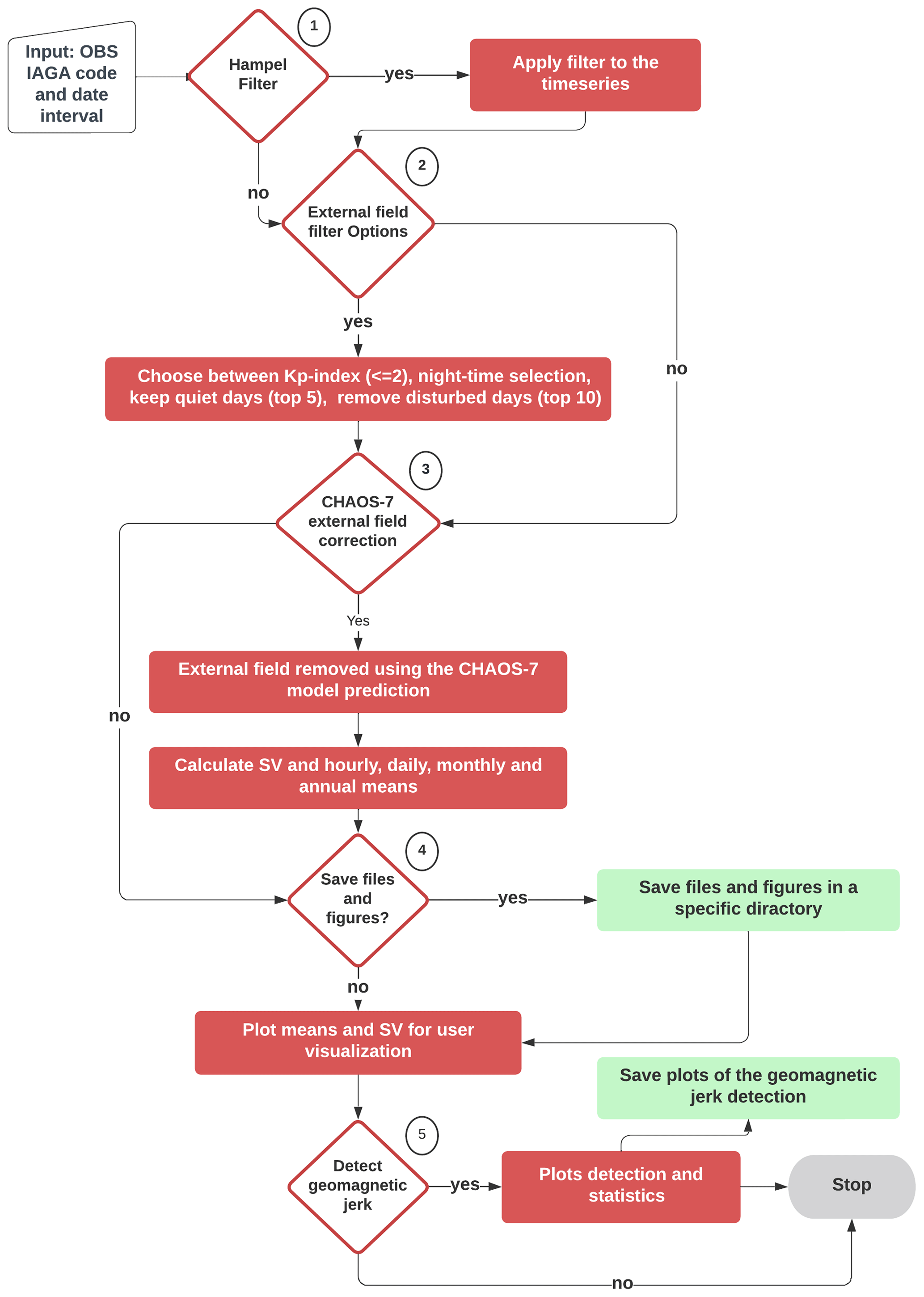
Figure 1 Flowchart of MOSFiT processing example as implemented in the interactive function sv_obs. The diamond shapes are the data processing sequence interactions, where the user chooses the options for data processing. Diamonds, red boxes, and green boxes represent user selections, processing steps, and output, respectively.

3 Description of methods

3.1 Outlier detection – Hampel filter

The Hampel filter is a robust outlier detector for time series; see Hampel (1974) and Pearson et al. (2016) for a detailed explanation. It is based on the median absolute deviation (MAD), since the MAD is less affected by outliers than the mean. Equation (1) is the M, where x_i is the ith observed data point and m the median for each window.

$$\begin{array}{}\text{(1)}& M=\mathrm{median}\left(|x_i-m|\right)\end{array}$$

It works like a sliding window over the time series. The filter sensitivity depends on the window size (number of samples) and the threshold (in multiples of standard deviation). Any data point exceeding the threshold is flagged as an outlier and replaced by the window median value. This approach follows the Cox et al. (2018) method of denoising the WDC data. By default, MOSFiT takes a window of 100 h and a threshold of 3 times the standard deviation. This choice is based on trial and error, and according to our visual inspection of SV time series it works well for most observatories. However, for some observatories other value combinations might work better.

3.2 External field reduction by data selection

One method to mitigate external field contributions is by selecting periods of low geomagnetic activity (Kauristie et al., 2017). In MOSFiT you can select periods of low Kp index or the international quiet days or exclude data from the international disturbed days. There is often a trade-off between stringent criteria retaining only a small amount of data and less stringent criteria that keep more external field affects in the data. Another method is to select nighttime, as the E-region (the E-region is a ionospheric layer at about 110 to 130 km altitude) ionospheric conductivity is then very low. Data selection is not only useful for studying the SV but also for ionospheric studies (Yamazaki and Maute, 2017) and internal field modeling (Kauristie et al., 2017).

3.2.1 Kp index

The Kp is a 3 h range index that is widely applied to data selection in geomagnetic field modeling and for studies of the ionosphere and magnetosphere (Kauristie et al., 2017). It is distributed by GFZ-Potsdam (https://kp.gfz-potsdam.de/en/, last access date: 11 October 2023); see Matzka et al. (2021) for a recent description of K and Kp index derivation. Selecting periods with Kp≤2 (default in MOSFiT) retains on average 30 % of the available data (Yamazaki and Maute, 2017), but as this depends on the position in the solar cycle and during periods of high solar activity, the Kp limit might have to be increased in order to retain a sufficient number of data. The function automatically downloads updated Kp index values from the GFZ website when the function is used. Figure 2 illustrates the MOSFiT Kp index selection function for Kp≤2 applied to Vassouras (VSS) data from January 2010 to May 2022.

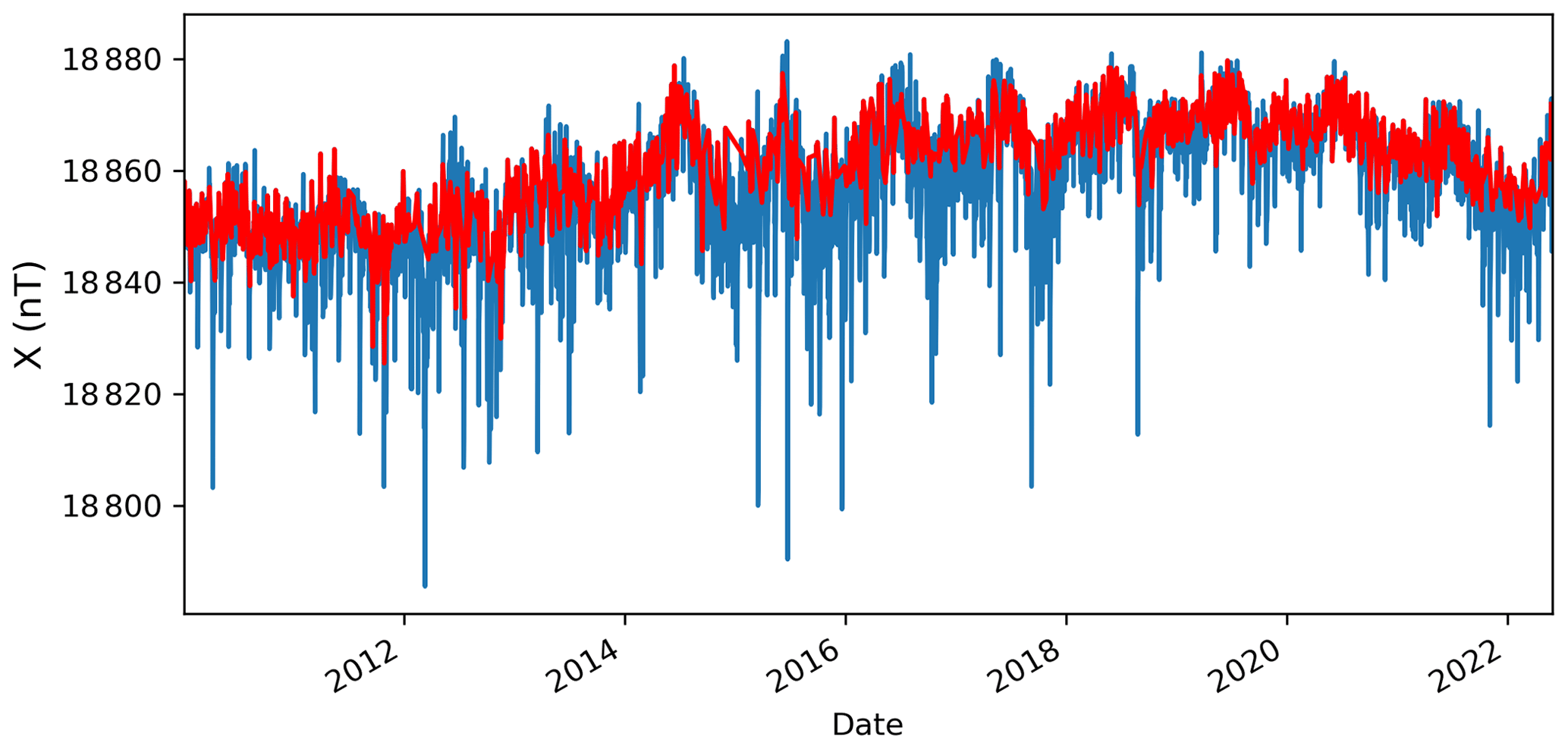
Figure 2 North geomagnetic field component (x) from Vassouras geomagnetic observatory (VSS). Daily means for all days (blue curve) and daily means for days with Kp index ≤ 2 calculated by the MOSFiT package (red curve).

3.2.2 International quiet days and international disturbed days

The international quiet days and international disturbed days (IQDs and IDDs, respectively) are derived from the Kp index and distributed by the GFZ-Potsdam on a monthly basis at https://www.gfz-potsdam.de/en/Kp-index (last access date: 11 October 2023). MOSFiT provides options to select data based on IDDs or IQDs, which completely remove the top 10 IDDs and keep the top 5 IQDs for each month of the dataset. Similar to the Kp index, the IDD and IQD lists are updated automatically when accessed by the package.

3.2.3 Nighttime selection

Nighttime geomagnetic data are less affected by overhead ionospheric E-region currents, e.g., the (daytime) Sq current system. This is due to the low E-region conductivity at nighttime. However, depending on the latitude of the station, other current systems can have effects during nighttime. For example, the substorm current wedge can affect sub-auroral data at around local midnight (McPherron et al., 1973; McPherron and Chu, 2017). The default value for nighttime selection in MOSFiT is from 22:00 to 02:00 LT (local time).

3.3 CHAOS-7 model correction

The CHAOS-7 geomagnetic field model (Finlay et al., 2020) is derived from Swarm, CHAMP, Orsted, and SAC-C satellite and ground observatory data. It predicts the contributions from the following sources: core, crust and magnetosphere. The MOSFiT package includes the version CHAOS-7.10, spanning from 1999 until August 2022 (see http://www.spacecenter.dk/files/magnetic-models/CHAOS-7, last access: 11 October 2023, for CHAOS release information).

The inputs are geodetic longitude and colatitude, distance to the Earth's center, timestamps for which the field will be predicted, and the ring current (RC) index (see below). The model output is the radial, colatitude and azimuthal component (B_r, B_θ and B_ϕ, respectively) for each geomagnetic field source, converted to the local XYZ coordinate system that is used for geomagnetic observatories.

The time-dependent core field is calculated up to spherical harmonic degree 20 and the static crustal field is calculated up to degree 110. Magnetospheric fields are calculated in the geocentric solar magnetospheric (GSM) and solar magnetic (SM) coordinate systems, with both being calculated up to degree 2 and with hourly resolution. They can be subtracted from the observatory hourly mean data in order to reduce external field influence. In order to calculate the SM contributions, MOSFiT is automatically updating the RC index from http://www.spacecenter.dk/files/magnetic-models/RC/current/ (last access: 11 October 2023).

Figure 3 compares the SV calculated for Kakioka geomagnetic observatory (KAK) before and after subtraction of the CHAOS-7 magnetospheric (GSM and SM) contribution. Additionally, Fig. 3 presents the SV calculated from the time-dependent CHAOS-7 core field prediction. Such a comparison demonstrates the better characterization of the SV after the filtering, explained by the good agreement with the predicted SV. Figure 3 shows that mostly the X component SV is influenced by the magnetospheric field and that its reduction by the CHAOS model significantly improves the SV information in the observatory time series.

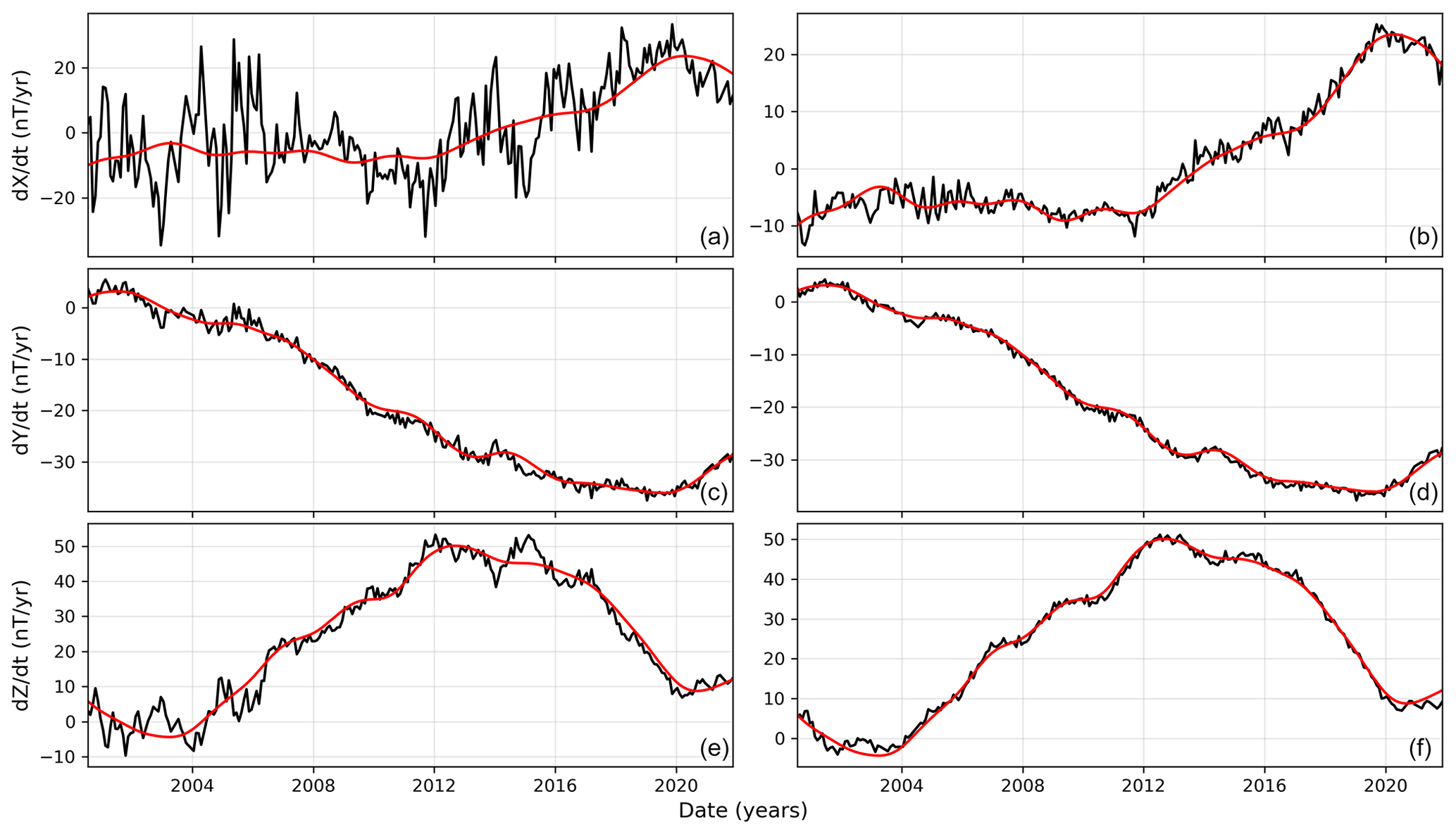
Figure 3 Kakioka magnetic observatory (KAK) secular variation (SV, black curves) calculated by MOSFiT before (a, c, e) and after (b, d, f) subtraction of magnetospheric field as predicted by CHAOS. SV calculated from CHAOS core field predictions are shown as red line.

3.4 Data resampling

The package can resample geomagnetic data as hourly, daily, monthly and annual means that are centered to the middle of the time interval. By default, MOSFiT calculates a mean value if at least 90 % of data are available (St-Louis and INTERMAGNET Operations Committee and Executive Council, 2020). For example, to resample from minute means to hourly means it is necessary to have a minimum of 54 individual minute means within this UT hour. The default can be disabled by the user, when the observatory has low data availability or to avoid cascading effects, for example if a few missing minute mean values cause a missing hourly mean values, which in turn causes some missing daily mean values and so on.

3.5 Secular variation calculation

The MOSFiT default method to calculate the SV at a time t is the monthly mean differences between t+6 months and t−6 months (Chulliat et al., 2010; Feng et al., 2018), known as the annual differences of monthly means (ADMM). Equation (2) represents the SV, where t is time in months and B is the magnetic field of any geomagnetic component. In most cases, monthly means are calculated from minute means (IAGA-2002, definitive and quasi-definitive data). Monthly means are a better option than annual means for SV investigations as they allow us to identify abrupt changes in SV trends in more detail. Importantly, this approach also reduces external field contributions by filtering out the seasonal variation from magnetospheric and ionospheric currents. Note that the solar quiet ionospheric currents are not modeled by CHAOS-7 and could otherwise introduce strong seasonal artifacts in the SV record (Mandea et al., 2000).

$$\begin{array}{}\text{(2)}& {\displaystyle \frac{\mathrm{d}B}{\mathrm{d}t}}=B_{(t+\mathrm{6})}-B_{(t-\mathrm{6})}\end{array}$$

3.6 Geomagnetic jerk detection

Geomagnetic jerks can be viewed as a sudden change in the first time derivative (SV) trend, characterized by a V-shaped pattern in the SV, or an abrupt change in the second time derivative (secular acceleration, SA) of the magnetic field. Usually, they are not observed simultaneously around the globe, i.e., the same event is observed shifted by several months at different observatories (Courtillot et al., 1978; Bloxham et al., 2002; Pinheiro et al., 2019).

Different methods to detect geomagnetic jerks have been applied in the literature, and Brown et al. (2013) give an overview of detected events, used data and detection techniques, of which the most common were least-squares fitting of two straight lines (Le Mouël et al., 1982; Le Huy et al., 1998; Pinheiro et al., 2011), wavelet analysis (Alexandrescu et al., 1996) and visual detection (Mandea et al., 2000; Olsen and Mandea, 2007; Chulliat et al., 2010).

MOSFiT provides an automatic fitting of two straight-line segments by least squares in a user-specified time window. This requires that the user chooses a suitable time interval that contains a jerk surrounded by two linear segments. The package makes use of PWLF (Jekel and Venter, 2019), a Python library that fits continuous piecewise linear functions to one-dimensional (1D) dependent variables. In our case, we want to fit two linear segments to the data without prescribing their intersection point, which is the geomagnetic jerk occurrence time (t₀). Global optimization is used to find the best intersection (t₀) by minimizing the sum-of-square error of the residuals. The detection is individually applied to the X, Y and Z components. The PWLF also gives the coefficient of determination (R²) and the slopes of the first and second segments. The jerk amplitude (A) is the slope of the second segment minus the slope of the first segment (Le Mouël et al., 1982; Pinheiro et al., 2011).

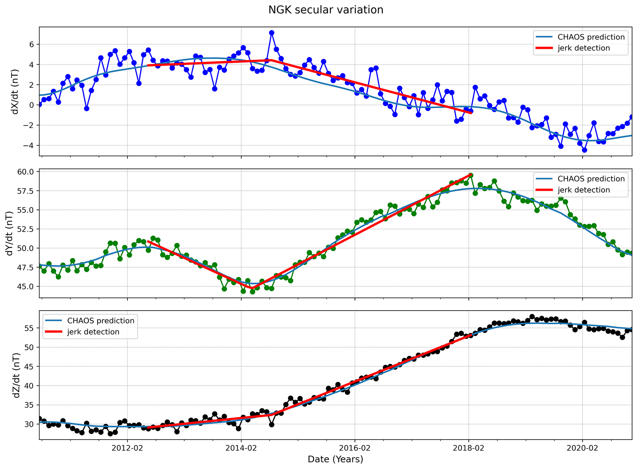
Figure 4 Niemegk geomagnetic observatory (NGK) SV. Dark blue, green and black are the SV for x, y and z geomagnetic components, respectively. Light blue lines give the SV from the CHAOS-7 predicted core field. The red lines show the linear segments identified by MOSFiT and indicate the start and end time of the user-selected detection window (June 2012 to January 2018).

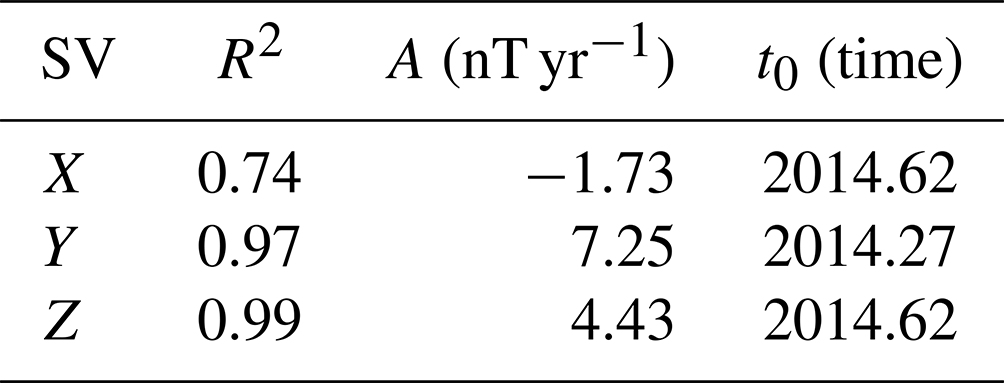
Figure 4 demonstrates the detection of the geomagnetic jerk in 2014 at Niemegk geomagnetic observatory (NGK) corrected by the CHAOS-7 magnetospheric field. The detection algorithm was applied to a time window from June 2012 to January 2018. The statistics about the detection are listed in Table 1. As expected, the SV in X has the largest misfit (R²=0.74) since it is the most affected by the external field contribution. The SV in Y and Z show a very good fit (R²=0.97 and 0.99, respectively). The occurrence time t₀ was identical for the X and Z component (2014.62) and about 4 months earlier in the Y component (2014.27). The user should be aware that the chosen detection window may affect the jerk characterization and should only select windows that contain visually clear changes in trend in the SV. Otherwise, the automatically determined jerk occurrence time and amplitude can be less accurate or wrong. The algorithm always fits two linear segments into the time chosen window, even if no apparent jerk signs exist. It is a user's task to interpret the results by, for example, setting a criteria to exclude jerks with lower R² values.

Table 1 Statistics of MOSFiT geomagnetic jerk detection for the jerk in 2014 at Niemegk magnetic observatory secular variation. The parameters R², A and t₀ are the coefficient of determination, jerk amplitude and occurrence time, respectively.

4 MOSFiT package validation

4.1 Case study 1: global misfit with and without magnetospheric correction

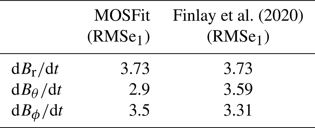
Finlay et al. (2020) calculated the rms misfit between the SV of CHAOS-7 magnetospheric corrected data of 181 magnetic observatories and the SV determined from the CHAOS core field. Their mean misfit for B_r, B_θ and B_ϕ is given in Table 2. We denote this method as RMSe₁ and repeat this exercise with MOSFiT on data from 115 INTERMAGNET observatories from January 2000 until June 2022. Our results (also in Table 2) are very similar though not identical as there are some differences in the observatories, time interval and CHAOS model version. They indicate that the CHAOS implementation in MOSFiT works properly. In Fig. 6 we show the global distribution of this rms misfit for the individual observatories. As expected, the largest misfits are observed at high latitudes, where the strongest unmodeled external field variations can be found. The smallest misfits are observed in Europe, likely because here the density of geomagnetic observatories is the highest.

Finlay et al. (2020)

Table 2 Validation of the MOSFiT implementation for external field correction by CHAOS-7 against results from Finlay et al. (2020).

In addition, we calculate the rms difference between SV determined from uncorrected geomagnetic observatory data and SV determined from the CHAOS-7.11 core field. We denote this method as RMSe₂ and show global mean values for high, middle and low latitudes in Table 3. It also shows the corresponding results for RMSe₁ and the percentage of improvement from RMSe₁ to RMSe₂. Figure 5 compares SV for X at Chambon-la-Forêt magnetic observatory (CLF) for different processing methods (blue), i.e., Kp selection, quiet days selection, nighttime selection and CHAOS correction, with the SV prediction by CHAOS. It clearly shows that the magnetospheric correction by CHAOS shows much closer similarity with the CHAOS SV prediction than data selection processing methods, which all give SV time series that are quite similar to that of the original data with the full content of external fields.

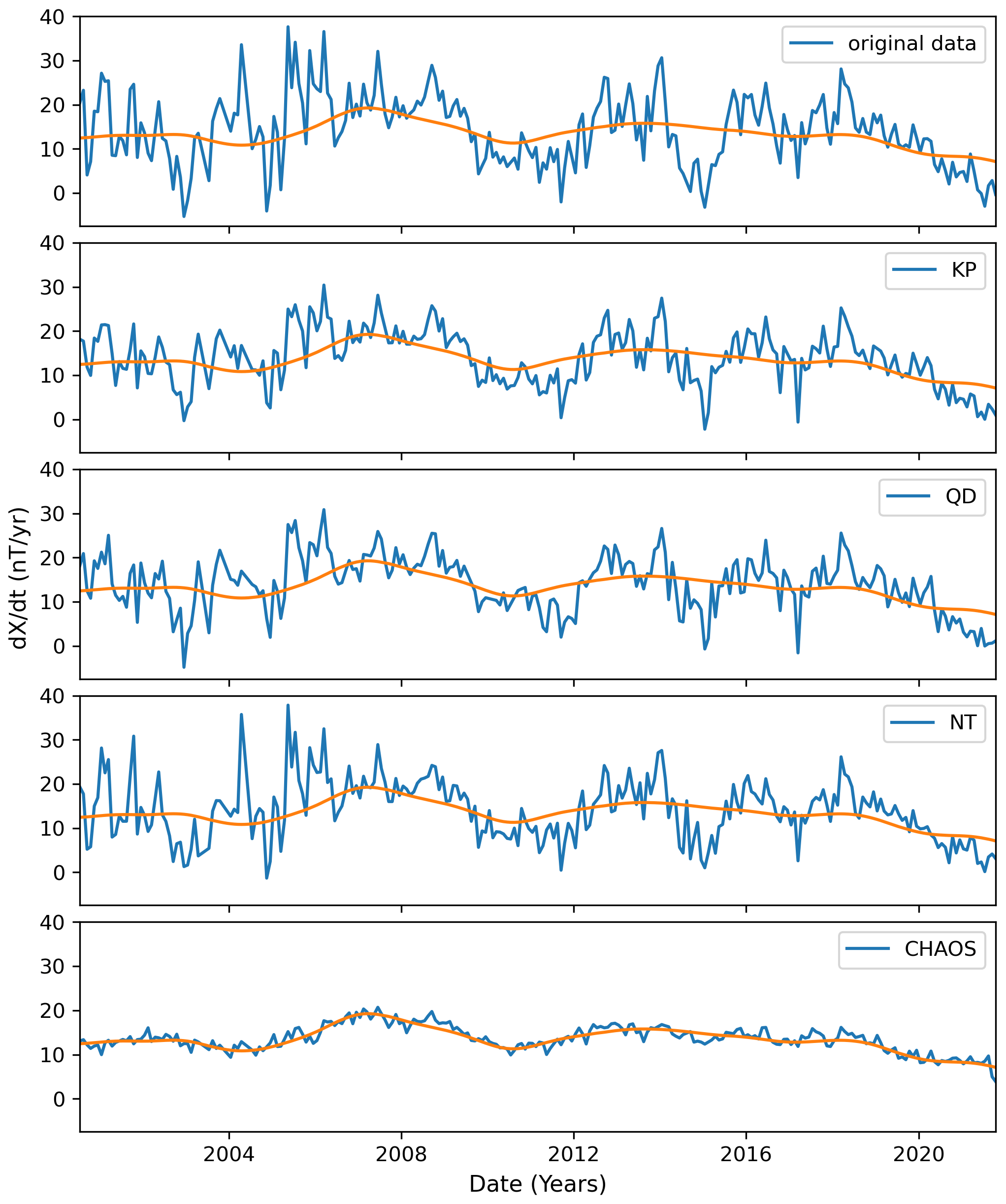
Figure 5 Chambon-la-Forêt geomagnetic observatory (CLF) x SV calculation using the processing methods KP, QD, NT, and CHAOS and original data compared to CHAOS-7 core field.

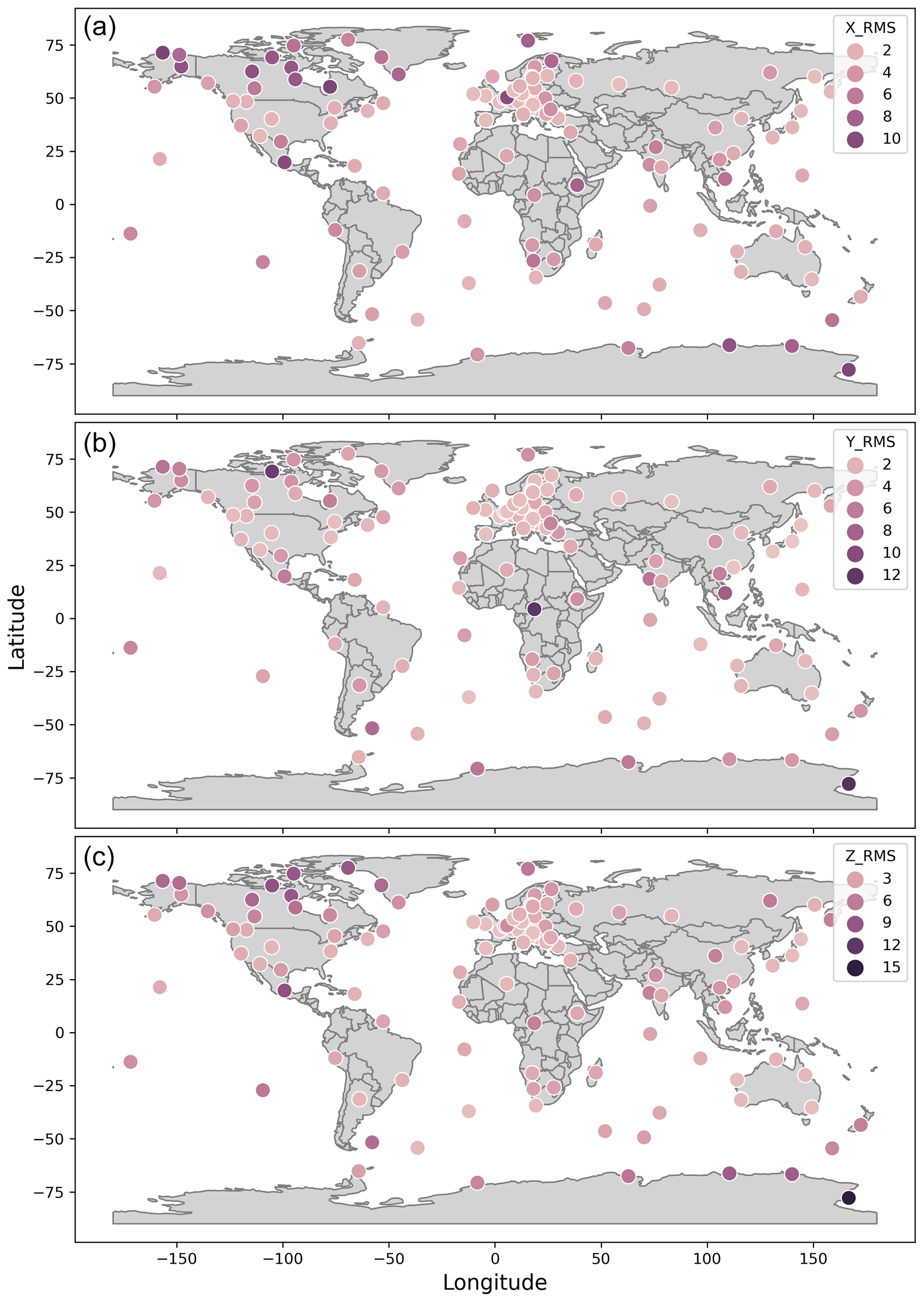
Figure 6 World map for X SV RMSe₁ from INTERMAGNET observatories. INTERMAGNET observatory RMSe between CHAOS-7 model internal field prediction SV and observed (filtered) SV. Maps of X, Y and Z SV from the top to the bottom, respectively. These results were produced by using MOSFiT package.

Table 3 CHAOS-7 model external field filtering effectiveness. Percentage of change between RMSe₂ and RMSe₁ (see text) for low, middle and high latitudes for the SV of the X, Y and Z component.

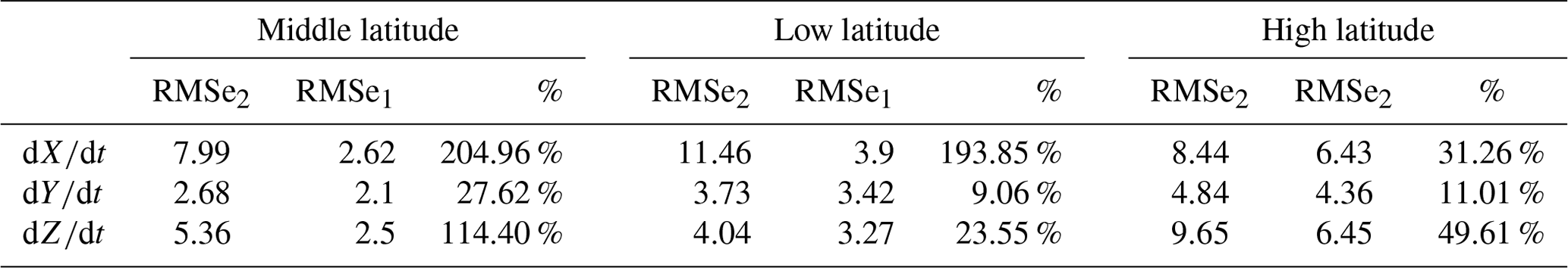
The most improvement is seen for $\mathrm{d}X/\mathrm{d}t$ at middle and low latitudes as the magnetospheric signal, which is modeled by CHAOS-7 and then subtracted, is strongest in the X component. At high latitudes the improvement is only around 30 % since signals from the auroral electrojet and field-aligned currents are not modeled by CHAOS-7. The Y component is least affected by external fields and shows the lowest rms values and the smallest improvements.

4.2 Case study 2: detection of the geomagnetic jerks in 2007, 2011 and 2014

In order to validate the MOSFiT methods, we automatically detected the jerks of 2007, 2011 and 2014 using observatory data from NGK, EBR, TAM and ASC. For the sake of comparison, we use methods similar to those described by Torta et al. (2015), i.e., only the y component without data selection or subtraction of external fields. Like Torta et al. (2015), we use only the data until the end of 2014. In Table 4 we compare MOSFiT results for occurrence time (t₀) and amplitude (A) with that of Torta et al. (2015). Additionally, we give the coefficient of determination (R²) and the user-specified start year and month, as well as end year and month, for the detection window. The detection window was selected visually from the SV plot based on the characteristic V shape and then repeated until the best misfit was achieved. Figure 7 shows the SV (blue dots), CHAOS-7 model SV prediction (green curves) and jerk detection (red lines) results of MOSFiT package.

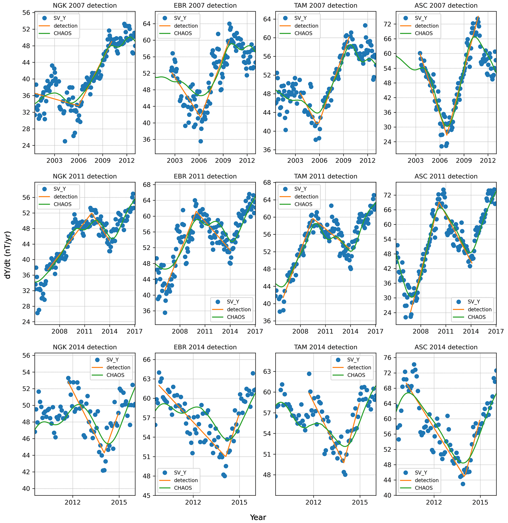
Figure 7 Geomagnetic jerk detection of the 2007, 2011 and 2014 events using the MOSFiT automatic method for NGK, EBR, TAM and ASC. Blue dots are the non-filtered Y component SV, green lines are the CHAOS-7 model internal field SV prediction and the straight orange lines are the MOSFiT automatic jerk detection.

Table 4 MOSFiT detection of geomagnetic jerks in 2007, 2011 and 2014 at the NGK, EBR, TAM and ASC observatories. Occurrence time (t₀) and amplitude (A) are shown for MOSFiT and for Torta et al. (2015) in parentheses. The coefficient of determination R² and the start and end year and month of the detection window are also shown for this study.

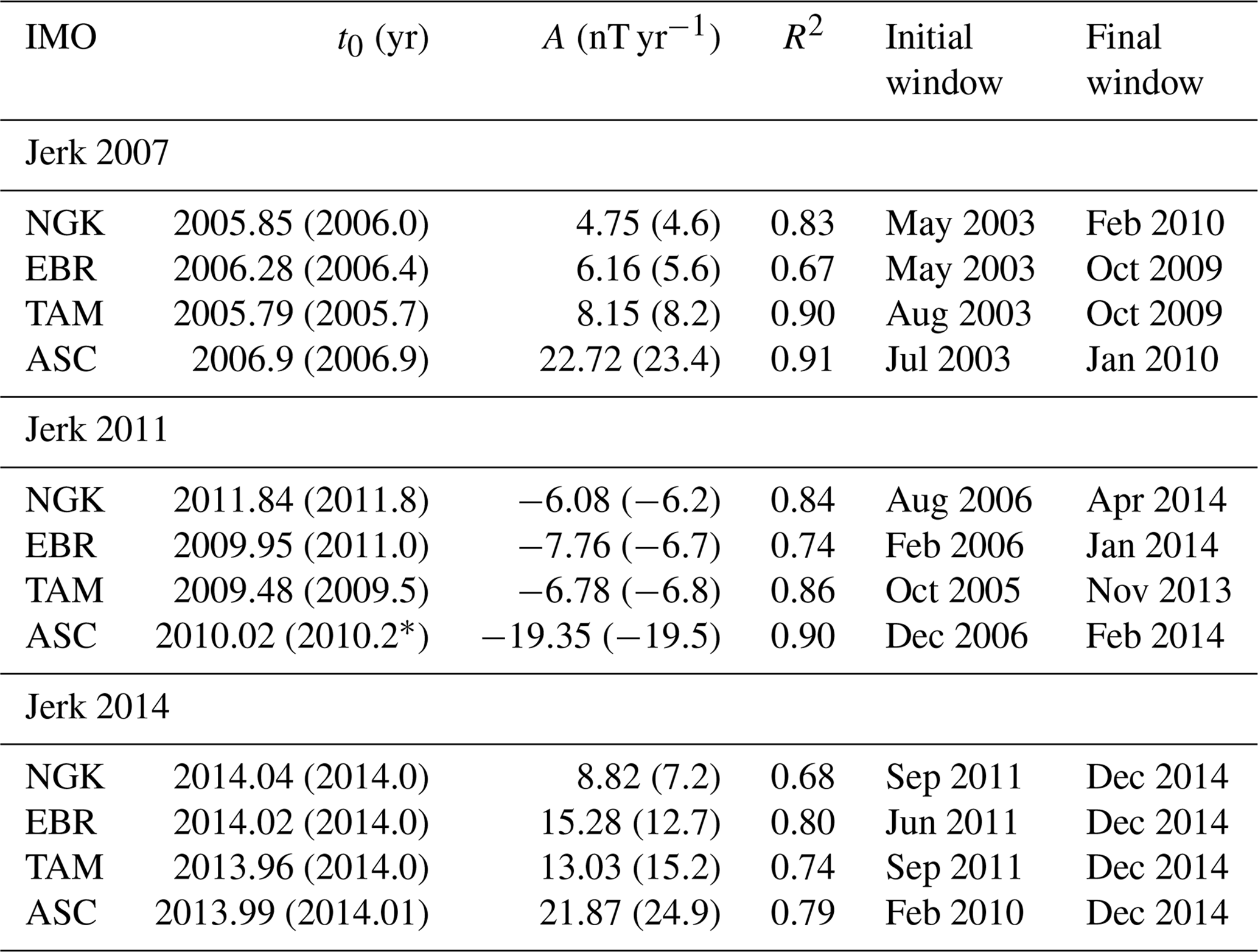
^* In Torta et al. (2015), the occurrence time of the 2011 jerk at ASC is misspelled as 2012.0 but should read 2010.2 (Joan Miquel Torta, personal communication, 2023).

The largest occurrence time difference between MOSFiT and Torta et al. (2015) for the jerk in 2007 is 0.15 years or 55 d for NGK, while the amplitudes are very similar. Jerk amplitudes detected by MOSFiT are very similar to those published by Torta et al. (2015). Finally, for the jerk in 2014 the results show a very good agreement for the occurrence time of the jerk and a good agreement for the amplitude at all four observatories.

5 MOSFiT application: determining the influence of the external field filtering methods on geomagnetic jerk detection

To evaluate the influence of different processing methods, i.e., no data selection and no CHAOS correction (original data), Kp data selection (later labeled KP), IQD data selection (labeled QD) and nighttime data selection (labeled NT), and the CHAOS-7 magnetospheric field reduction (labeled CHAOS), we selected 10 globally distributed INTERMAGNET observatories (Fig. 8) to analyze the 2007, 2011 and 2014 jerks in the X, Y and Z components.

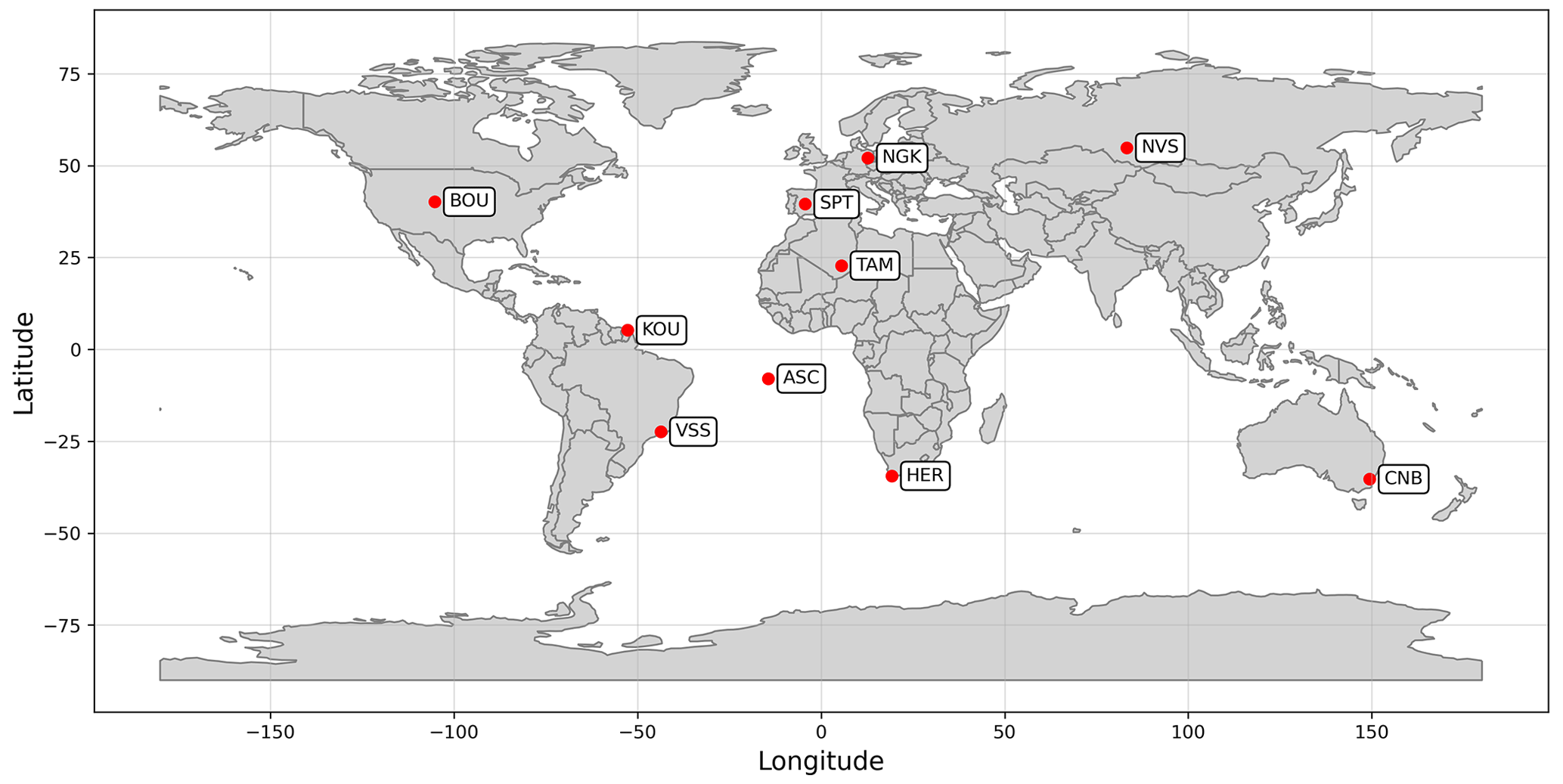
Figure 8 INTERMAGNET observatories used in the application for determining the influence of the external field filtering methods on geomagnetic jerk detection. The three-letter IAGA code indicates the observatory.

The detection window was individually chosen according to the range of the SV trend for each of the observatories but always remained the same for the different processing methods. For each processing method the occurrence time (t₀) and the amplitude (A) were determined.

In this analysis, only jerks with high values of R² are considered that have the typical “V” shape in their SV (note that in NVS and CNB in 2007 did not show the V-shape, for example) and that were detected by all processing methods. A total of 24 jerks were detected in the Y component, 22 in the Z and only 7 in the X. Note that a total of 12 jerks in the X component were only detectable after using the CHAOS-7 magnetospheric reduction, which shows how important this correction is.

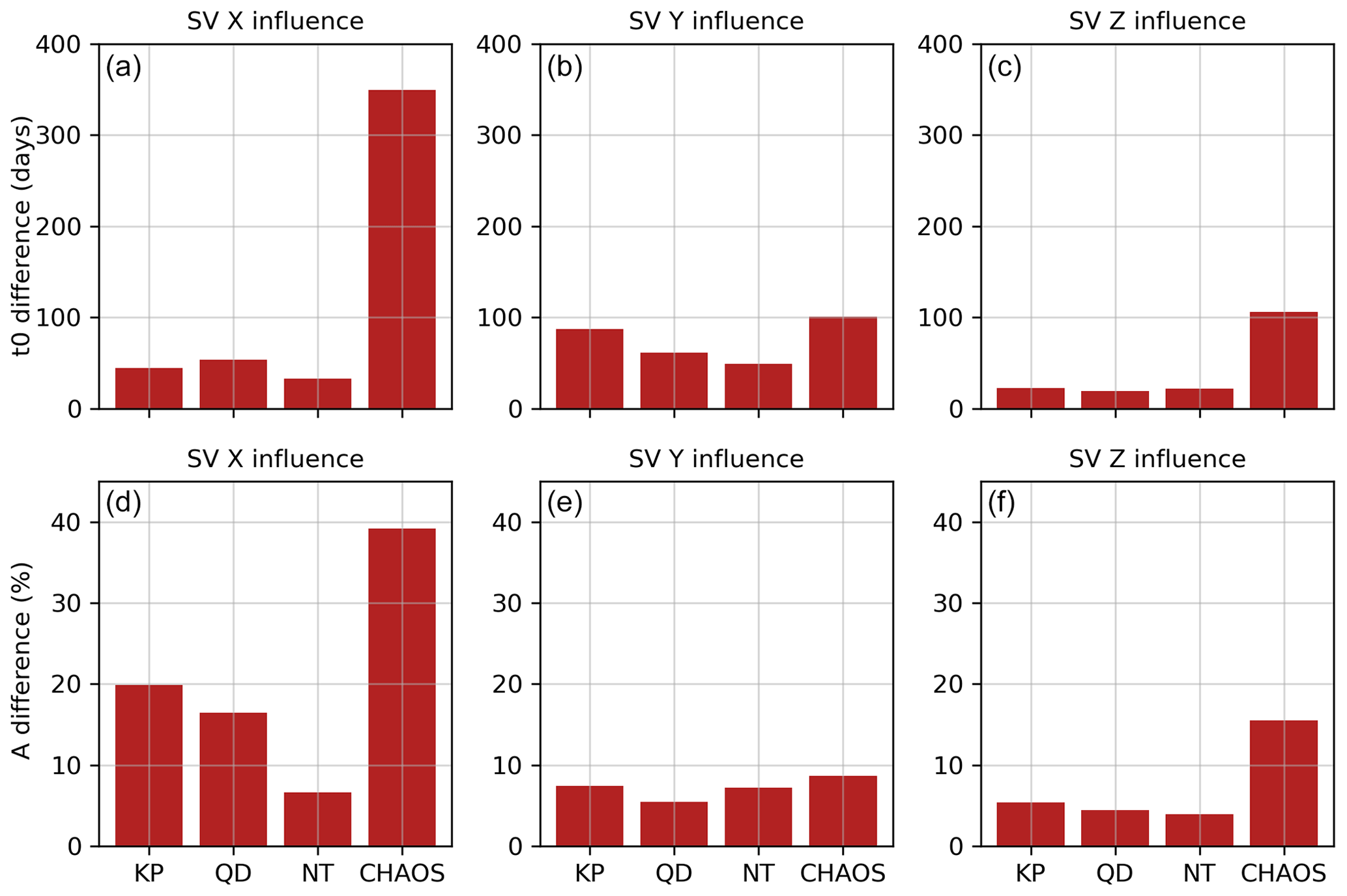
Figure 9 (a–c) Mean absolute difference in jerk occurrence time Δt₀ in days between processed data and original observatory data for different processing methods KP, QD, NT and CHAOS (for an explanation, see Sect. 5) for X, Y and Z. (d–f) The same as the upper panels but for jerk amplitude difference (ΔA) in %.

The upper panels in Fig. 9 show the mean of the absolute difference in jerk occurrence time (in days) of the processing methods KP, QD, NT and CHAOS compared to using the original data. The mean occurrence time (Δt₀) difference between CHAOS correction and the original data is largest for the X component (349 d), where it is about 7 times larger than for the processing methods KP, QD and NT (44, 53 and 33 d, respectively). A similar pattern is seen for Z, where CHAOS gives 105 d, which is about 5 times larger than KP, QD and NT (23, 19, 22 d, respectively). From this comparison alone one cannot define if the CHAOS magnetospheric correction is either a lot better or a lot worse in these components than the data selection methods tested. However, given that the ring current has a strong amplitude combined with fast temporal changes compared to a jerk and that its signal is not removed by nighttime or Kp-dependent data selection, one can expect that it is the magnetospheric correction that performs best.

For the Y component (Fig. 9b) the absolute shift in t₀ is similar for all processing methods with CHAOS changing in terms of t₀ the most (by 100 d) and NT changing the least (by 50 d). For the jerk amplitude difference (given as a percentage in the lower panels in Fig. 9), we observe a similar pattern to that of occurrence time t₀.

6 Conclusion

We present the Python package MOSFiT (Magnetic Observatory and Stations Filtering Tool) to investigate the geomagnetic secular variation (SV) in observatory data. MOSFiT is designed to work with 1 min INTERMAGNET definitive and quasi-definitive data. However, it can also be applied to any geomagnetic observatory or magnetometer data. The package offers outlier rejection (Hampel filter), four data selection options (quiet days, disturbed days, Kp index and nighttime period) and a magnetospheric field reduction using CHAOS-7. MOSFiT can resample the data to hourly, daily, monthly and annual means and provides a method to determine geomagnetic jerk occurrence time (t₀) and amplitude (A). All steps can be visualized. We successfully validate the implementation of CHAOS in MOSFiT against results for more than 150 observatories presented by Finlay et al. (2020) and the MOSFiT geomagnetic jerk detection method against results for three jerks (2007, 2011, 2014) presented by Torta et al. (2015). We investigate the difference between the observatory data SV and the CHAOS core field SV (by calculating its rms) for uncorrected and observatory data corrected by the CHAOS magnetospheric field prediction for 115 geomagnetic observatories in low, middle and high latitudes. For the uncorrected observatory data, this difference is smallest in the Y component. The magnetospheric field correction reduces this difference most strongly (by about two-thirds) in the X component in low and middle latitudes. In general, the differences after the magnetospheric correction are similar for the X, Y and Z components and similar to the difference for the uncorrected Y component. We further quantified the effect of different observatory data processing methods on the determination of the jerk occurrence time (t₀) and the jerk amplitude (A) for the three jerks for a subset of 10 geomagnetic observatories and found that the CHAOS magnetospheric correction performs best, especially for the X and Z component. MOSFiT is available at https://github.com/marcosv9/MOSFiT-package (last access: 11 October 2023), and we expect it can be a great help for geomagnetic observatory data analysis, allowing convenient and automatic access to the most recent geomagnetic observatory data and indices. In particular, it will allow a timely identification of any future geomagnetic jerks and can be used as a tool for geomagnetic observatory data quality control.