Auroral alert version 1.0: two-step automatic detection of sudden aurora intensification from all-sky JPEG images

A sudden and significant intensification of the auroral arc with expanding motion (we call it “local-arc breaking” hereafter) is an important event in many aspects but easy to miss for real-time watching due to its short rise time. To ease this problem, a real-time alert system for local-arc breaking was developed for the Kiruna all-sky camera (ASC) using ASC images in the JPEG format. The identification of the local-arc breaking is made in two steps using the “expert system” in both steps: (1) explicit criteria for classification of each pixel and simple calculations afterward are applied to each ASC image to obtain a simple set of numbers, or the “ASC auroral index”, representing the occupancy of aurora pixels and characteristic intensity of the brightest aurora in the image; (2) using this ASC auroral index, the level of auroral activity is estimated, aiming for Level 6 as clear local-arc breaking and Level 4 as a precursor for it (reserving Levels 1–3 for less active aurora and Level 5 for less intense sudden intensification).

The first step is further divided into two stages. Stage (1a) uses simple criteria for R (red), G (green), and B (blue) values in the RGB color code and the H (hue) value calculated from these RGB values, each pixel of a JPEG image is classified into three aurora categories (from brightest to faintest, “strong aurora”, “green arc”, and “visible diffuse (aurora)”) and three non-aurora light source categories (“cloud”, “artificial light”, and “Moon”). Here, strong aurora means that the ordinary green color by atomic oxygen's 558 nm emission is either nearly saturated or mixed with red color at around 670 nm emitted, by molecular nitrogen. In stage (1b), the percentage of the occupying area (pixel coverage) for each category and the characteristic intensity of the strong aurora pixels are calculated.

The obtained ASC auroral index is posted in both an ASCII format and plots in real time (https://www.irf.se/alis/allsky/nowcast/, last access: 11 April 2023). When Level 6 (local-arc breaking) is detected, an automatic alert email is sent out to the registered addresses immediately. The alert system started on 5 November 2021, and the results (both Level 6 detection and Level 4 detection) were compared to the manual (eye) identification of the auroral activity in the ASC during the rest of the aurora season of the Kiruna ASC (i.e., all images during a total of 5 months until April 2022 were examined and occasionally double-checked in the sky). Unless the Moon or the cloud blocks the brightened region, a nearly one-to-one correspondence between Level 6 and eye-identified local-arc breaking in the ASC images is achieved with an uncertainty of under 10 min.

1 Introduction

In space weather monitoring and real-time studies of the ionospheric and/or magnetospheric science, real-time broadcasting the monitoring results of the local geomagnetic and ionospheric conditions (i.e., nowcasting) is as important as monitoring the upstream conditions. Here, the upstream condition includes the solar wind and the interplanetary magnetic field (IMF) conditions at the Sun–Earth Lagrange (L1) point and the detection of a coronal mass ejection (CME) and a solar flare at the Sun. Although the upstream monitor provides predictions of global activities, it is difficult to predict and impossible to know the local geomagnetic and ionospheric activities with the upstream monitor only. This difficulty applies even when the local activity is part of the predicted global activity, such as a substorm: even these cases have uncertainties of at least more than 30 min and several degrees in latitude and longitude. This means that the location and timing of high geomagnetic and ionospheric activity are difficult to predict under these uncertainties, particularly for events with a high risk of space weather hazards. For such local forecasts, monitoring the local condition (such as the geomagnetic field and all-sky camera (ASC) images) and comparing it with upstream conditions and regional conditions (the area covered by several stations) are essential.

Here, the auroral condition is known to reflect the magnetospheric and ionospheric conditions (e.g., Akasofu, 1977), and the hazardous magnetospheric/ionospheric conditions almost always cause intense and enlarged aurora. This is why many high-latitude observatories started nowcasting the local auroral conditions (e.g., webcasting the real-time data) after relevant technology became ready. Even data from regional networks of observations such as the geomagnetic array (Friis-Christensen et al., 1988; Luhr et al., 1998) and the ASC array (Syrjäsuo et al., 1998; Partamies et al., 2003) are being nowcasted, updating every minute or even more frequently.

Among many traditional methods to monitor the local auroral condition, cost and technical difficulty of the ASC decreased drastically during the past 3 decades, making the ASC (including those using consumer cameras) the most convenient method to monitor the ionospheric condition, although its operation is limited to night. Figure 1 shows an example of the aurora image taken by the Kiruna ASC that uses the consumer camera (archive is found at https://www.irf.se/alis/allsky/krn/yyyy/, last access: 11 April 2023). In addition to the ASC images, some observatories nowcast the keograms of these ASC images using the north–south slices of the images (see Fig. 2 for the explanation of the keogram). These data are normally archived in the JPEG format with a red–green–blue (RGB) color code (a world-standard image compression format).

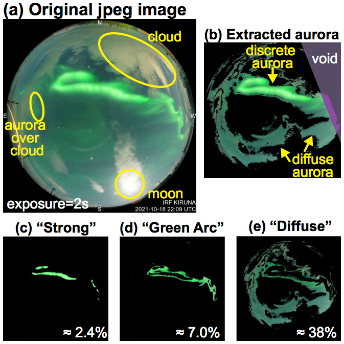
Figure 1 The all-sky image and processed images of 18 October 2021, 22:09 UT, taken by the Kiruna all-sky camera (ASC). The automatic exposure time for this particular image is 2 s (second-shortest due to the Moon). Aurora pixels are characterized by green color (its emission is at the 558 nm wavelength, but that is not resolved in the RGB system). (a) ASC image before the analysis (low-resolution JPEG with 482×482 pixels) that is shrunk from the original image (2832×2832 pixels). Basic categories of aurora (discrete and diffuse), cloud, and the Moon are marked in the figure. (b–e) Processed images by the automatic identification of each pixel (present method), extracting (b) all aurora pixels (window is 430×430 pixels), (c) only the “strong aurora” in the present definition, (d) only the “green arc”, and (e) only “visible diffuse”. In the analysis, we mask all pixels at more than 215 pixels from the center and also the upper right corner (purple-shaded region in b) because this part is normally contaminated by city light (located to the west of the ASC).

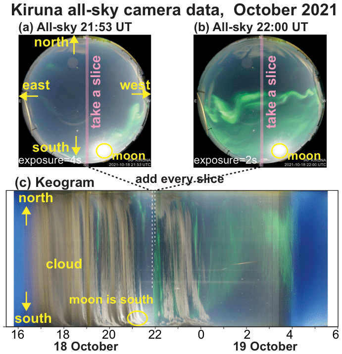
Figure 2 An example of the keogram that is created from a time series of the all-sky camera (ASC) images. Panels (a) and (b) show the ASC images during the “local-arc breaking” (see text for explanation): (a) 21:53 UT with 4 s exposure and (b) 22:00 UT with 2 s exposure. Only the north–south slice of each image (red shaded area in the middle) is used to create (c) the keogram, a time series of the activity (but with a mixed exposure times) seen in the north–south meridian.

The usability of the ASC also stimulated non-specialists of the aurora to use the ASC data. These potential users include electric power companies, the satellite community (scientists, engineers, and operators) except those engaged with optical instruments, and even tourists and aurora enthusiasts. However, these potential users are normally not familiar with interpreting the ASC aurora images or keograms. For example, different aurora forms (the ratio of different types of the aurora) mean different magnetosphere–ionosphere current systems for different conditions, such as different UT and different phases of the aurora cycle (about 1–2 h). Understanding these differences requires background knowledge of the relationship between various auroral conditions and various magnetospheric/ionosphere activities in addition to actually watching the aurora with the naked eye (Akasofu, 1977). Thus, judging the auroral condition is more demanding than judging the simple morphological difference (no existing machine-learning method has overcome this problem; see Discussion section). Considering a wide range of possible users, it would be ideal if the traditional manual evaluation of auroral activity were translated to a numerical scheme and nowcasted in addition to the keograms.

As the first step of such a translation, we define a number representing the size or intensity of each light source (e.g., aurora, Moon, cloud). Such a set (short list) of numbers, namely the ASC auroral index, is similar to the geomagnetic indices (obtained from multi-station data) such as the auroral electrojet (AE) by the World Data Center (WDC, 2022) in Kyoto (nowcast site: https://wdc.kugi.kyoto-u.ac.jp/ae_realtime/presentmonth/index.html, last access: 11 April 2023) for the aurora region and Kp by the Helmholtz Centre Potsdam – German Research Centre for Geoscience (GFZ, 2022) in Potsdam (nowcast site: https://isdc.gfz-potsdam.de/kp-index/, last access: 11 April 2023) for the sub-aurora region. Another analogy is the moment data (density, velocity, pressure) calculated from a particle spectrometer. Such an “index” allows even specialists to gain an overview of the activity during the most recent 1 h through line plots of the index values.

In both the geomagnetic indices and moment values, these simplified “numbers” are used to judge the level of geomagnetic and plasma activities. Likewise, the ASC auroral index can be used to evaluate the auroral activity level, such as the sudden and significant intensification of the auroral arc with expanding motion (we call it “local-arc breaking” hereafter). This part is again the translation of eye identification of the activity level (e.g., Akasofu, 1977) into a numerical value. This “second step” classification (judging the activity level from a set of numbers) opens up the possibility of the real-time alert of high activities including the local-arc breaking. The sequence of aurora images shown in Figs. 2a, b, and 1a (21:53, 22:00, and 22:09 UT, respectively, on 18 October 2021) is an example of the local-arc breaking, as characterized by a quick and expanding northward motion of the brightest green aurora. The motion is also recognized in the keogram (Fig. 2c). Such a real-time alert even allows automatic switch to burst-mode monitoring with a higher resolution (e.g., every 5–10 s instead of every 1 min) to keep the archiving size as small as possible for non-essential periods.

In this paper, we describe our numerical translation of manual judgment by aurora scientists (expert system) to obtain the Kiruna auroral index and activity level from the all-sky image in Kiruna.

2 The Kiruna ASC and source JPEG images

The source data are JPEG images from the Kiruna ASC, which is operated by the Kiruna Atmospheric and Geophysical Observatory (KAGO) at the Swedish Institute of Space Physics (IRF). The ASC is located in a 30 cm heated dome at the roof of the optical laboratory, as shown in Fig. 3, in Kiruna at 68^∘ N. The viewing direction of the ASC image is given in Fig. 2a. From September 2020, the Kiruna ASC uses a Sony α7s (firmware rev 3.2) with a Nikon Nikkor 8 mm 1:2.8 objective fish-eye lens with the iris fully open. ISO is set to 4000, and the color temperature (white balance) is set 5000 K during the 2021/2022 winter season. The exposure time is dynamic from 1 s to about 30 s. Like the other standard digital cameras, this camera uses three CCDs (charge-coupled devices) with wide-spectrum coverage centered on red, green, and blue colors. The values of the intensity detected by each CCD compose the RGB color code.

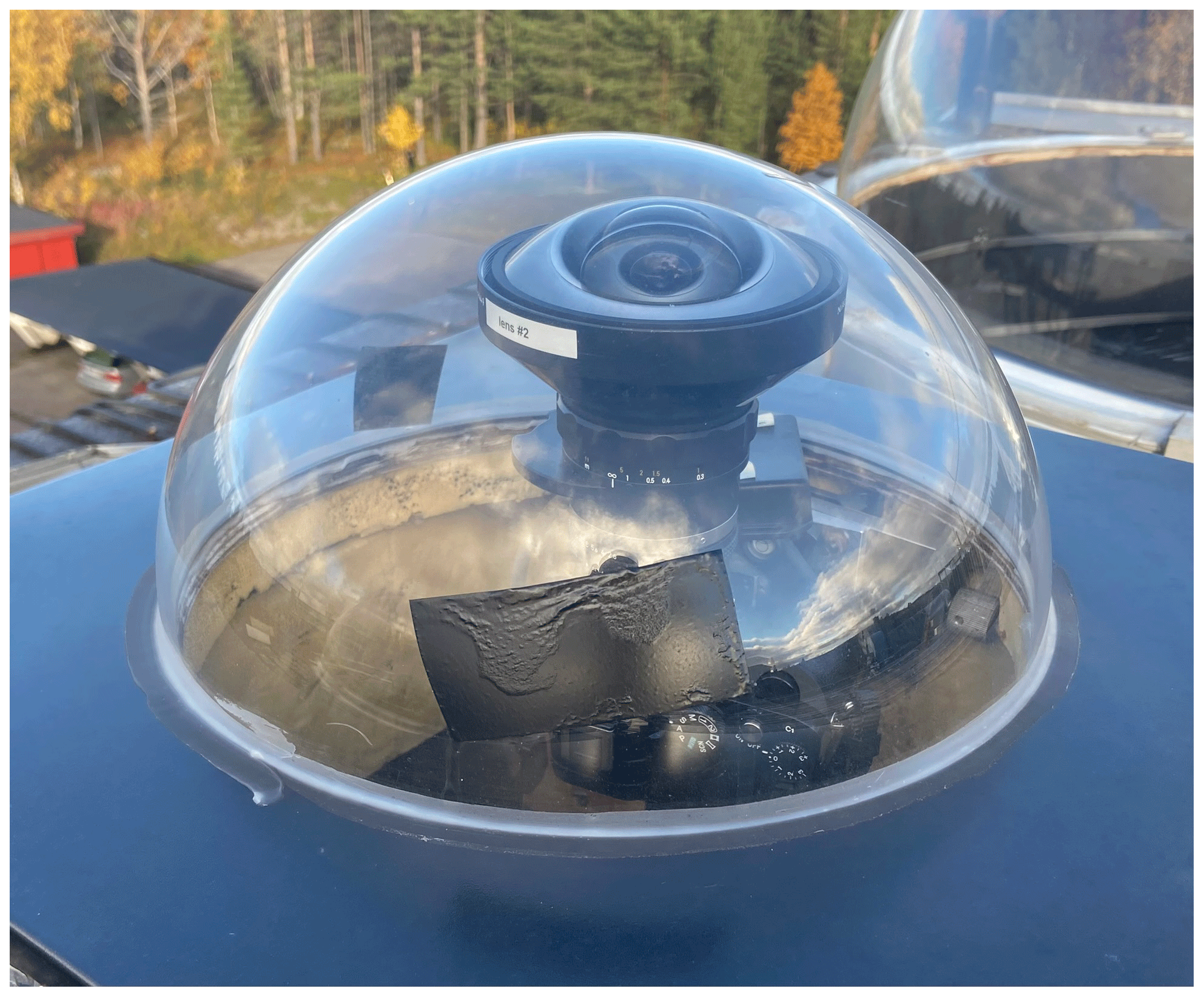
Figure 3 The all-sky camera (ASC) at the Swedish Institute of Space Physics in Kiruna (68^∘ N).

The camera is controlled by a Raspberry Pi 4 computer and set to produce RGB color-coded JPEG files (no raw data output due to storage space limitations), 2832×2832 pixels in size, of which a circle with a diameter of about 2700 pixels (about 5.7 million pixels) corresponds to the actual sky window. The data are stored on a disk server and made available in real time (https://www.irf.se/sv/observatorieverksamhet/firmamentkamera/, last access: 11 April 2023). In addition to the original JPEG files, JPEG files with a reduced resolution are also stored in the archive: medium-resolution JPEGs (924×924 pixels) and low-resolution JPEGs (482×482 pixels).

We use the low-resolution JPEG output, which has a size about the same as those obtained from the old camera (Nikon D700 camera, in service until April 2020). Using the smallest size of JPEG also saves computation time. Fortunately, the difference in the color values of each pixel between different JPEG formats (reduced-resolution JPEG compared to raw JPEG output from the camera) is much smaller than the difference in the color values between different cameras or during different light conditions (Moon, twilight, cloud) according to our experience. This is partly because the JPEG compression preserves aurora's green color well and is clearly different from the other light sources at night in the RGB space.

Since the JPEG format with the RGB color code is commonly used for ASC nowcasting, a successful algorithm for the Kiruna ASC may open up a possibility of application (with proper modification) to a wide range of aurora cameras, including those owned by schools and private sectors (e.g., Toyomasu et al., 2008). This would benefit science (event identification and clarification of physics behind the classification and evaluation), operations (archiving, satellite, space weather counterpart), and even education and tourism.

3 Algorithm

As mentioned in the introduction, there are two major tasks: (1) to obtain the ASC auroral index, i.e., a set of numbers representing the sky condition using the color information for all pixels (about 1.4×10⁵ pixels with a 3-byte color information each), and (2) to evaluate the activity level from this index. A successful result of part (1) should make part (2) easy.

The first task is further subdivided into two steps. (1a) We classify each pixel into different categories using mathematical criteria on the RGB values: three categories of aurora (“strong aurora”, “green arc”, and “visible diffuse (aurora)”, as shown in Fig. 1), non-aurora light sources (cloud, Moon, artificial light), and an unclassified category. To save computation resources, each pixel is classified independently without considering neighboring pixels' color, except for judging the Moon (white color occupies a solid small area with a radius of at least 5 pixels and often about 10 pixels). The classification scheme is detailed in Sect. 2.1–2.3. (1b) We calculate the coverage of each light source and characteristic intensity of the aurora pixels, as described in Sect. 2.4. For the second task (2), we define the activity level, such as the local-arc breaking, using only the index values, by applying a set of simple criteria, without using any pixel-level information, as described in Sect. 2.5.

To obtain the level, we do not need high digits for the index values, like the traditional eye identification of the aurora. Only one to two digits of accuracy for the occupancy area in each category (about 50 pixels for the strong aurora category and about 150 pixels for the green arc category, according to our experience) are sufficient in defining the activity level. This means that we do not need an exact one-to-one pixel level relation between the actual type of the aurora and the classification category. Such tolerance eases the problems related to the JPEG compression, such as the color difference between different JPEG compression schemes from the same image and only a 3-byte value (1 byte each for R, G, and B) for color information in each pixel.

The high tolerance also saves computation resources by classifying each pixel independently without considering neighboring pixels' color except for judging the Moon. Such a pixel-level identification of the aurora emission is possible partly because the most bright aurora emission for the human eye (558 nm) is quite different from other non-aurora emissions in the RGB color space.

3.1 Selection of aurora color

In version 1.0, we judge only the green aurora (558 nm), which is normally registered as high G values. However, using only the G value in the RGB system is misleading because any bright or white light sources (the Moon, artificial light, and cloud reflecting these lights) have a wide spectrum including the green color component, giving high G values. In fact, the human eye uses low values in the $\mathrm{R}/\mathrm{G}$ and $\mathrm{B}/\mathrm{G}$ ratios in addition to a high G value when distinguishing the green aurora from other light sources in the non-filtered ASC images. We first aim to translate such distinctions to a numerical scheme.

One useful parameter is the hue (H) of the hue–saturation–lightness (HSL) color code that is calculated from the RGB values. We can also use the lightness (L) to set the lowest threshold of aurora brightness. Using the calculated HSL values, we actually made a primitive version (version 0) of a real-time classification for the old ASC (Nikon D700 camera) from November 2016 to April 2020 (see Appendix A for the criteria). Although version 0 could identify many of the local-arc breakings (Yamauchi et al., 2018, a presentation at the EGU General Assembly), the HSL method causes many identification errors in the aurora pixels for the Sony camera that has been in use since August 2020. Therefore, we use all values of R, G, B, calculated H, and L.

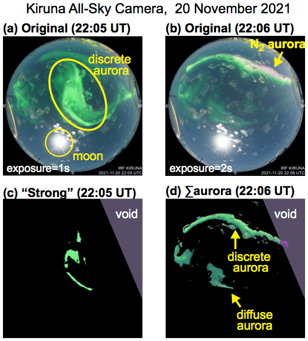
Figure 4 All-sky images of 20 November 2021 at (a) 22:05 UT with 1 s exposure and (b) 22:06 UT with 2 s exposure, in the same format as in Fig. 1a. (c, d) Processed images of (a) and (b) in the same format as in Fig. 1c and 1b, respectively. The bright spot is the Moon, which is removed during the processing.

Note that the H value of an aurora pixel significantly deviates from that corresponding to 558 nm even when the non-aurora emissions are ignorable, partly because other aurora emissions can be mixed. Just limiting the emission to the main visible ones, there are three colors that may mix with the green 558 nm emission: several red emission lines around 670 nm corresponding to the nitrogen molecule (N₂ red lines), a few blue emission lines near 428 nm corresponding to the molecular nitrogen ion (${\mathrm{N}}_{\mathrm{2}}^{+}$ blue lines), and different red emission line at 630 nm corresponding to the atomic oxygen (O red line). These emissions become strong when the activity is very high, particularly during the local-arc breaking.

Among these emissions, the N₂ red line (around 670 nm) often overlaps with the most intense part of the green aurora (558 nm), from different emission altitudes (N₂ red line from <100 km and oxygen green line from >100 km), resulting in the aurora color shifting significantly toward red (higher $\mathrm{R}/\mathrm{G}$ ratio). Similarly, the ${\mathrm{N}}_{\mathrm{2}}^{+}$ blue line increases the $\mathrm{B}/\mathrm{G}$ ratio (shifting the color toward blue). An example of the ASC image with the bright N₂ red line is shown in Fig. 4: strong red emissions are found next to (i.e., on the north side of) the main auroral arc in Fig. 4b. The white color at pixels between the red pixels and the green pixels is the result of both emissions overlapping each other on the same pixel. In this particular case, these pixels are not counted as the (green) aurora pixel simply because R ≥ G. Fortunately, these lines are intensified only when the green aurora is also intensified, and we can still judge most of such mixed-aurora pixels as strong aurora by increasing the criterion values for the $\mathrm{R}/\mathrm{G}$ value or the $\mathrm{B}/\mathrm{G}$ value for higher G ranges. Even the exceptional case like Fig. 4b is normally accompanied by a sufficient amount of the strong aurora pixels on the same image or images ±1 min as shown in Fig. 4 and does not affect the final evaluation of the auroral activity very much. Therefore, we do not include such strong N₂ red-line pixels as the aurora pixels in version 1.0.

There is another factor that affects the color in the RGB system during substorms (e.g., Akasofu, 1977): saturation of the G value of bright discrete aurora pixels. For such aurora pixels, non-saturated R and B values increase for higher activity, causing a significant increase in the $\mathrm{R}/\mathrm{G}$ and $\mathrm{B}/\mathrm{G}$ ratios (while keeping G > R and R > B) and even causing deviation in the H value. The color shift (large departure of the H value from that corresponding to 558 nm) also comes from the contamination by non-aurora light sources, particularly the Moon and twilight, and the degree of this shift changes with the exposure time (generally shifting to red for a longer exposure time).

Fortunately, we may allow tolerance for the pixel-level classification as mentioned above, and handling of such color shifts is possible. Here, we prioritize the criteria for not misjudging the non-aurora source as strong aurora in a critical manner.

3.2 Pixel classification scheme

For the aurora pixel, we define three categories instead of two (discrete and diffuse) because the actual classification is fuzzy and often difficult to judge between discrete and diffuse. We can then define the strong aurora pixel only as a clear one. The green arc category is meant for the discrete aurora with less intensity, and the definition is inclusive because we do not like to miss the discrete aurora from the first two categories. Although such a definition may classify a strong diffuse aurora pixel as belonging to this category, this error is not critical in detecting the local-arc breaking because the strong aurora is mainly used in defining the local-arc breaking. The visible diffuse category is meant for only visible ones, while cameras can detect even weaker diffuse aurora emissions that the naked eye cannot normally recognize. In Fig. 1, the discrete part of Fig. 1a is recognized in Fig. 1c and d, while diffuse part of Fig. 1a is recognized in Fig. 1e.

Otherwise, the definition is exclusive; i.e., pixels with aurora but not meeting these criteria are excluded from our aurora pixels. We allow such false-positive cases because such a pixel normally includes aurora emissions through the cloud or under the influence of artificial light, and it is difficult to observe or to use for a scientific investigation anyway. We even dismissed weak diffuse aurora pixels as “dark” because that is not very important in diagnosing the activity level.

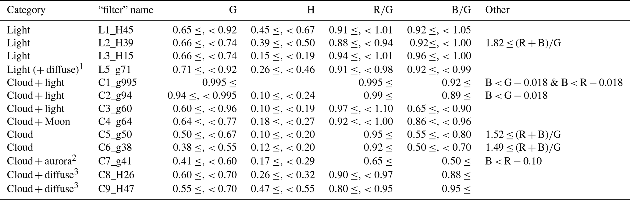
The exclusive definition is used even when defining the criteria for each category: we add small “safe” areas (we call them “filter” hereafter) in the RGB color space one by one with OR logic, as illustrated in Fig. 5. Since the color balance (H, $\mathrm{R}/\mathrm{G}$, and $\mathrm{B}/\mathrm{G}$) for the same category changes dynamically and nonlinearly for different G values, we make each filter as restrictive as possible to exclude colors that belong to the other category for the same G values. This method allows us to safely add a new criterion in case we miss some color range for the aurora pixel, while avoiding misjudging non-aurora emissions as aurora emissions. Furthermore, even the strong N₂ red line with a very little green line (see Fig. 4) can be added as a new category after separating its color code from the twilight.

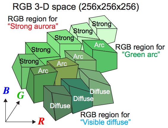
Figure 5 Schematic illustration of how the criteria of aurora pixels are constructed in the RGB color space. Each small box represents one of many criteria for one category (we call them “filter” in this paper) that we consider safe to judge as the aurora. By adding these “safe” criteria (with OR logic), we can cover a wide range of color (shifted from 558 nm) as the aurora. The block shape is not necessarily rectangular because we use G, $\mathrm{R}/\mathrm{G}$, $\mathrm{B}/\mathrm{G}$, and H in different ways for different criteria. The exact conditions are given in Table 2. Such a restrictive definition allows the possibility of adding more pixels to be identified as the aurora pixels, such as pixels dominated by the N₂ red line (Fig. 4).

The final shape of the RGB color area for the aurora pixels is not smoothly connected, i.e., not completely accurate, as illustrated in Fig. 5. With such uncertainty, some colors simultaneously belong to different categories (e.g., aurora and cloud), while some colors do not belong to any category even if the relevant pixel does not necessarily belong to the clear sky without aurora (such as dark cloud near the edge of the image that does not have enough reflection). However, these uncertainties are not a problem in defining the activity level, for which high tolerance is allowed in the auroral index values as mentioned above.

The exact criteria of the aurora pixels (strong aurora, green arc, visible diffuse) are obtained by manual tuning of the condition. Here, the RGB values of each pixel are extracted after we manually classified the pixel. Table 1 shows an example list of RGB values of pixels for different categories that are manually evaluated (by eye) for Fig. 1a. By examining several different pixels for the same category, we can make a list of R, G, and B values for one category for one image. This is repeated for different categories (even including the Moon and cloud), different times, different phase of a local-arc breaking (before, during, and after), different local-arc breakings, other types of auroral activities, and different days with different conditions (e.g., Moon, cloud, twilight). Once the values are obtained, we also calculate the H, L, $\mathrm{R}/\mathrm{G}$, $\mathrm{B}/\mathrm{G}$, and (R + B)$/$G values.

Table 1 Example of manual classification and color values of pixels from an ASC image (18 October 2022 at 22:09 UT, exposure time = 2 s; Fig. 1a).

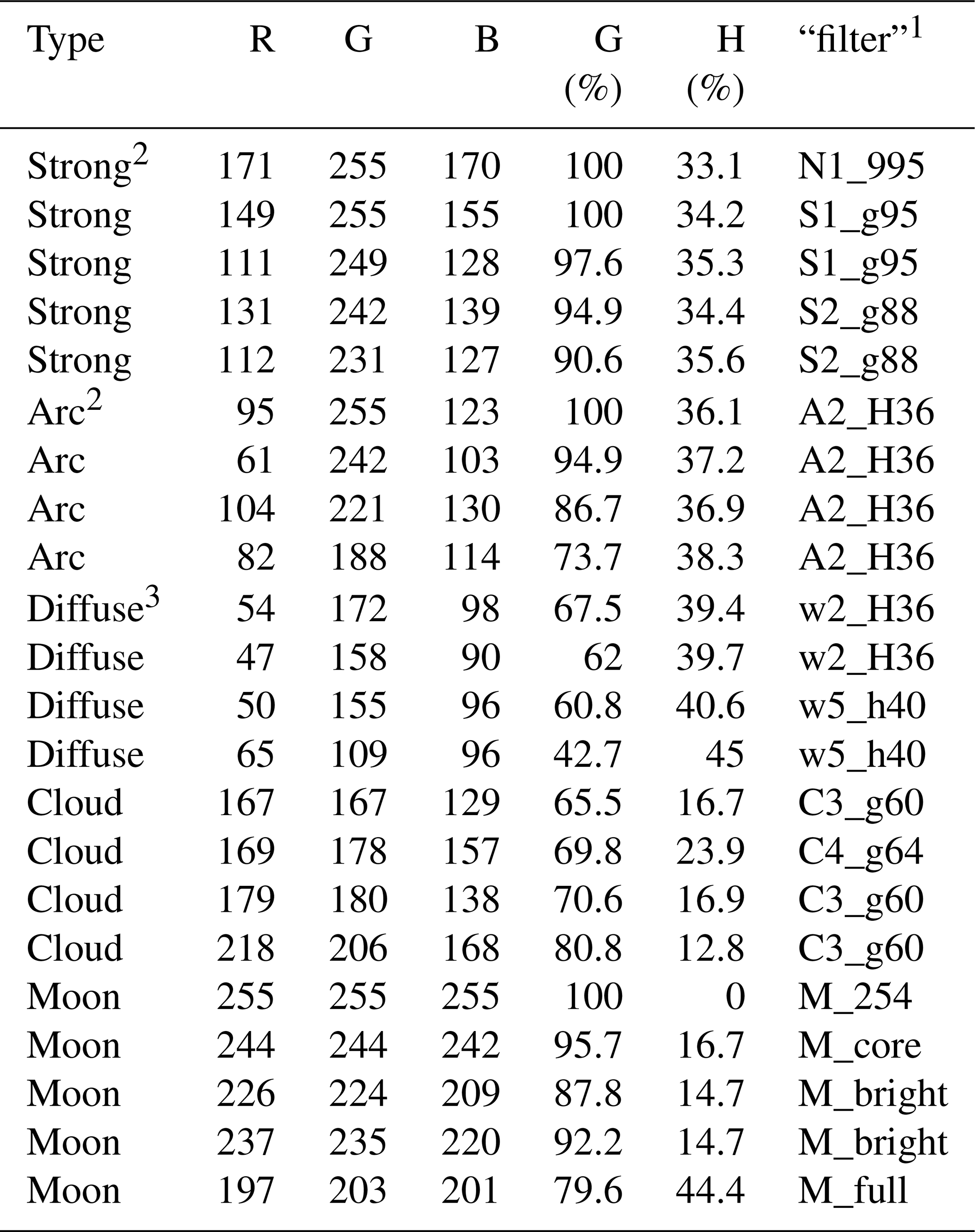
¹ Each filter means a set of criteria (see Fig. 5) that is defined in Tables 2–4. ² Reconstruction of “strong”, “arc”, and “diffuse” is shown in Fig. 1c, d, and e, respectively. ³ A diffuse aurora pixel is always weak (“w”) to the naked eye.

After completing the list for all samples, we arrange the list in terms of G and H values for each category such that we can tune the condition for other values for a given range of the G value (and H value). We prioritize G and H values because these two values are determining factors of how close to green the color is, respectively.

3.3 Actual pixel-color criteria for each category

The result for the Kiruna ASC is given in Table 2 for aurora pixels. The criteria are given with AND logic between columns (each row constructs one filter, named S1, S2, S3, and so on) and then OR logic between rows. The exact values of the criteria are camera-dependent, but the deviation of the values for different cameras would generally move toward higher or lower values of R, G, B, and therefore the modification will not be very difficult for aurora scientists who actually operate the ASC.

Table 2 Criteria of a pixel for the strong aurora, green arc, and visible diffuse categories (“strong”, “arc”, and “diffuse” in the first column, respectively).

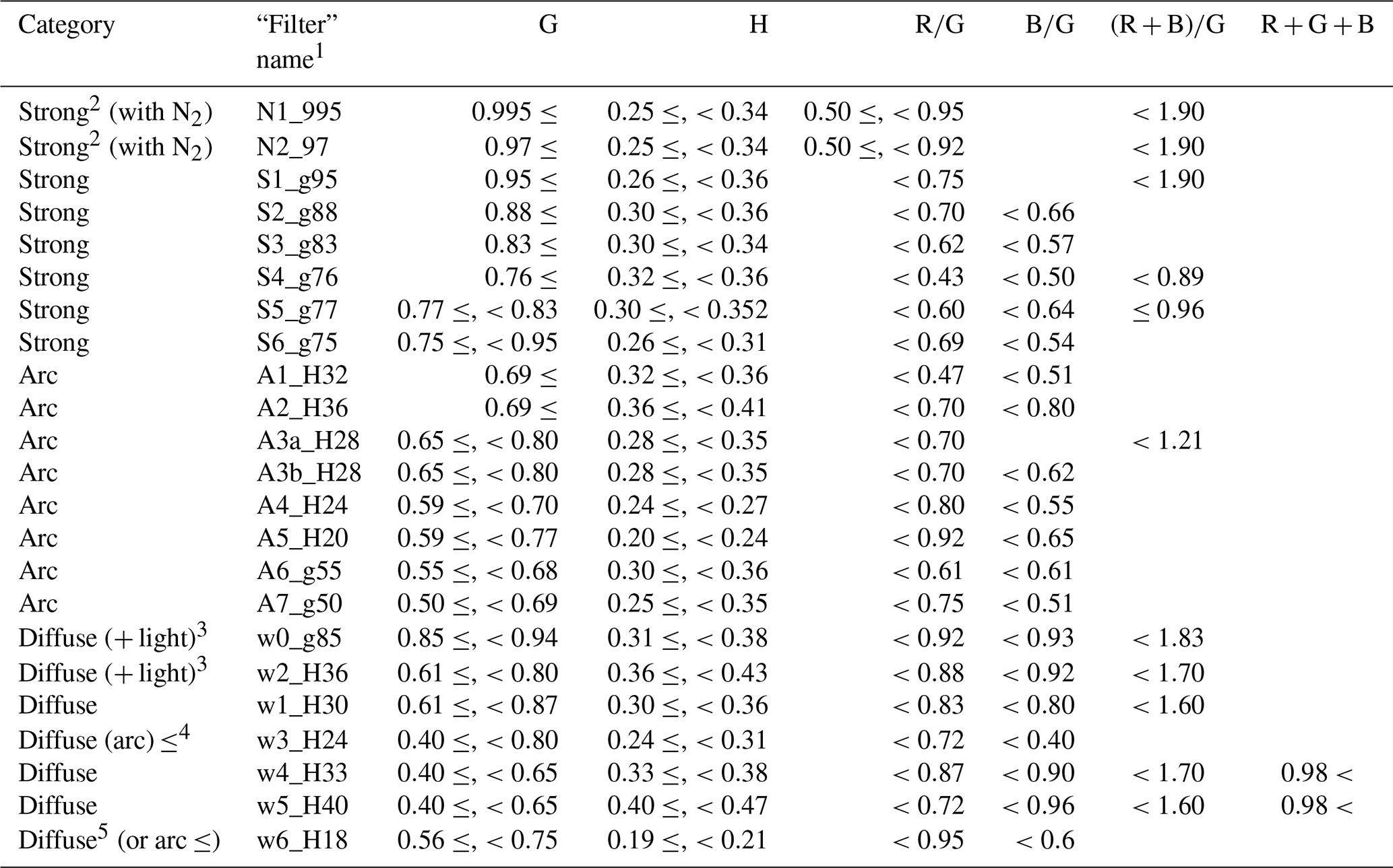
¹ The name of a filter (a criterion) that can pick up specific color ranges of the aurora pixel, and the final criterion for each category is a summation of different filter under OR logic. ² Contamination from the N₂ red line (about 670 nm; see text) increases the $\mathrm{R}/\mathrm{G}$ value. ³ Contamination by light is recognized, but most likely a visible aurora pixel. ⁴ Structured diffuse aurora. ⁵ It could belong to the green arc that is reflected by a cloud or seen through a cloud, but we remain on the safe side by not including the arc.

Table 3 Criteria of a pixel for the Moon and its surrounding (the same format as Table 2).

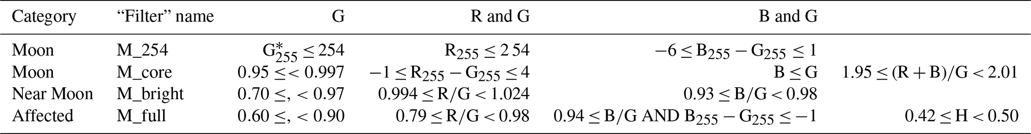
^* R₂₅₅, G₂₅₅, and H₂₅₅ are JPEG value of R, G, and B (0–255 instead of 0–1), respectively.

Criteria for pixels with non-aurora emissions are derived in the same manner as for the aurora pixels. Table 3 shows the results for the “Moon” and its surroundings, and Table 4 shows the results for artificial “light”, “cloud” with or without the aurora (too thick to judge). As mentioned above, the body of the Moon (characterized by high values of all of R, G, B because of its wide color spectrum) is obtained from the image as a densely populated solid region of pixels (radius of at least five pixels) that satisfy the Moon criterion. We decided not to use the Moon location calculated from time and the Moon orbit because the Moon location is displaced by the dome, and the Moon is often hidden by cloud, making the part of sky that is not covered by cloud less affected by the Moon (the main problem of the Moon is its effect on the dome rather than on the sky color).

Table 4 Criteria of a pixel for artificial light (“light” in the first column) and cloud (the same format as Table 2).

¹ Similar to note 3 in Table 2, but the light effect is stronger than that of the diffuse aurora. ² The green arc or strong aurora is above the cloud. ³ The diffuse aurora is above the cloud.

In these classifications, some pixels meet two or more different definitions. Therefore, we also give a priority order in the following:

1. the Moon (Table 3) and artificial light (Table 4),

2. strong aurora (Table 2),

3. green arc (Table 2),

4. visible diffuse (Table 2), and

5. cloud (Table 4).

The reason for the first priority is to avoid false-negative alerts (overestimation of aurora pixels) because a false negative occurs more easily than a false positive. Even with such a restrictive definition to avoid a false negative, a false negative happened as often as a false positive from our empirical experience. As compensation, very strong aurora pixels (such as those completely saturated with the N₂ red line in Fig. 4) can be judged as the Moon or artificial light, but this is a minor problem thanks to the high tolerance (allowing 50–150 pixels out of about 1.4×10⁵ pixels to be misjudged) and the reason given at the explanation of the N₂ red line. Fortunately, most of the very strong aurora pixels (e.g., G = 1.0) that are mixed with the other aurora emissions have safe H values (0.24 < H < 0.34) and are identified as belonging to the green arc or the strong aurora category.

The priority order for 2, 3, and 4 is obvious: among all “possibly aurora pixels”, we select aurora pixels, and out of them we select auroral arc pixels (the rest is visible diffuse), and from the auroral arc we select the strong aurora pixels (the rest is green arc). The cloud comes as the last priority because this is for estimating the active area, and a thin cloud allows strong aurora to penetrate through it. In practice, the majority of the cloud criteria do not overlap with the aurora definition.

Related to the Moon, there is another problem: the Moon modifies the color toward higher L and higher $\mathrm{B}/\mathrm{G}$ values at almost all pixels (even aurora pixels far away from the Moon) due to the refraction of the dome. This modification is larger at pixels closer to the Moon. While a better solution for the Moon problem (e.g., making the criteria different for different exposure times) will be considered in future, we reduce the Moon effect by simply masking all pixels within a certain distance from the Moon pixels (14 times the Moon radius that is dynamically obtained) for the present version 1.0. Outside this masked region, the Moon effect is moderate; i.e., the diffuse aurora will never be classified as belonging to the strong aurora category, and even the green arc is not easily classified as belonging to the strong aurora category.

Of course, such masking may cause an underestimation of the number of pixels of the strong aurora within this masking distance, although the eye can identify them. Such a coincidence actually happens because the Moon is normally located in the south, where the local-arc breaking sometimes takes place in Kiruna. Fortunately, after 5 months of real-time operation, the number of missed local-arc breaking due to this coincidence is small (cf. Sect. 3.5) because the aurora often expands beyond the masked region after the local-arc breaking (we have enough samples of local-arc breaking under moonlight). Thus, the present version of dealing with the Moon is still effective. Since the Moon is characterized by high values of all of R, G, and B, our Moon mask would work at other latitudes.

We also imposed another mask (void region) at the northwest edge where both artificial green light source and strong city light are within the field of view (purple-shaded area in Fig. 1). Since the light source only covers the area near the edge of the ASC's field of view, we simply remove the entire section from the analysis.

3.4 Calculation of the ASC auroral index

With the classification criteria for each pixel ready (Tables 2–4), we next obtain a set of numbers (parameters) representing the entire image. The obvious parameter is the number of pixels or, more precisely, the percentage of the coverage over the sky out of about 1.4×10⁵ active pixels after removing the void region (see Fig. 1b). Since we use a fish-eye lens (almost all ASCs use some sort of fish-eye lens), there are strong geometrical distortions, particularly near the horizon. Also, the distance to the emission region (strongest at 100–150 km) is strongly distorted near the horizon. Fortunately, both types of distortion are small near the zenith and can also be compensated for by deploying additional cameras. Therefore, we do not include any correction in the present version (v. 1.0). Including the geometrical effect is one of the future tasks.

The strong aurora (which means near saturation or mixture with the N₂ red lines) is normally identified in a small part of the sky, and the occupancy even during the local-arc breaking is normally only around 0.5 %–5 % (700–7000 pixels after looking at all plots for the value over 5 months). The green arc occupies a larger area (normally around 1 %–20 % during and before the local-arc breaking). For reference, strong aurora pixels in Fig. 1 occupy 2.4 % (3387 pixels out of 139 525 pixels) of the active area of the ASC. Here, local-arc breaking means the obvious expansion of the strong aurora (normally more than doubling in size within a few minutes). Considering a judging error in the strong aurora pixel of about 10 % (e.g., Fig. 1c compared to Fig. 1d) and less than 30 pixels of artificial green light that can be misjudged as the strong aurora, a significant number of 0.03 % or 40 pixels for the strong aurora and 0.1 % or 150 pixels for the green arc are sufficient in judging the activity level. For the other non-aurora categories, our identification accuracy of the occupied area is much worse, but still we obtain a significant digit of 0.1 %.

The obtained occupancy of the aurora pixels over the sky, however, is not sufficient in evaluating the activity level because it gives higher values for relatively less luminous aurora with a wide area than relatively more luminous aurora with a small area within the same category. Another problem is that the brightness given as L values in the HSL color code (L = (G + min(R,B))$/\mathrm{2}$ for aurora pixels with G > R, B) is not proportional to the photon counts (Brändström et al., 2012; Sigernes et al., 2014). Therefore, we also define the characteristic brightness of the aurora. Here, we do not take a simple summation of L over the aurora pixels because such a summation still gives higher values for large aurora areas with low L values than for a compact one with high L values. Instead, we obtain a kind of average intensity of the strong aurora pixels, as described below.

If the number of pixels of the strong aurora exceeds 4900 pixels (about 3.5 % of the image), we simply use the pixel data for the most luminous 4900 pixels (judged by the L value) of the strong aurora pixels. Here, the threshold number can actually be reduced for the present purpose, but it works anyway (as shown in the result below) and does not affect computation time. Afterward, we use a nonlinear scheme for averaging. We first take the average of both L values and L³ values. We reduce the obtained average values if the numbers of aurora pixels are small with the coefficient roughly proportional to $\mathrm{1}/\sqrt{n_{\mathrm{arc}}}$, where n_arc is the number of green arc pixels, and 0 when strong aurora pixels are less than 10. Here we use the L value as representing the luminosity, but we can use G values because what we are counting is the intensity of the green (558 nm) aurora. The exact Python code is found in the Supplement.

Table 5 summarizes the obtained parameters for the ASC auroral index. The index values are stored in an ASCII file in csv (comma separated value) format on a website in real time every minute (https://www.irf.se/alis/allsky/nowcast/, last access: 11 April 2023). The real-time plot and the archive of the past data are also found on the same website. For the ASCII file, we temporally made its width only 72 columns without a tab, which makes the file format very similar to the IAGA2002 format of the geomagnetic field. It is quite possible to extend the column to include other key parameters such as the exposure time, Moon position, and aurora position, but that will be a future task.

Table 5 Content of the ASC auroral index.

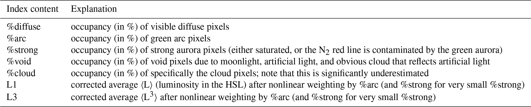
Figure 6 shows an example of comparison between the index values and the keogram over one night (11–12 March 2022). ASC images when the Level 6 activity is detected were also displayed at the bottom. One can see good correspondence with the index values and keogram image.

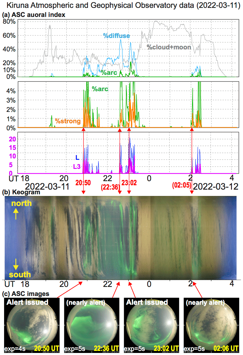
Figure 6 An example of (a) the ASC auroral index over one night (11–12 March 2022) with both active aurora and occasional cloud. As reference, (b) keogram over the same night and (c) all-sky images at the time of the auroral alert issued for Level 6 activities. Each image is taken toward the sky with north at the top, and hence east (west) is on the left (right). All images again include the Moon or Moon-brightened cloud. The automatic exposure time is 4 or 5 s for the displayed images.

Table 6 Criteria for the activity levels (same format as Tables 2–4).

3.5 Evaluation of the activity level from the ASC auroral index

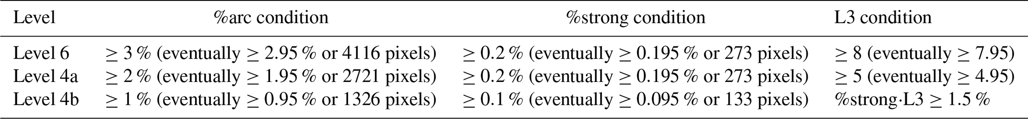
The next task is to evaluate the activity level from the index values without examining the image data and then to define the criterion for the activity level that corresponds to the local-arc breaking or, more exactly, a sudden and significant intensification of the auroral arc with expanding motion. Here, the “significant intensification” means high values of L1 or L3 (see Table 5 for definition), with the “expanding motion” accompanied by more than certain values of “%arc” and “%strong”. Table 6 summarizes the criteria for the activity level (Level 6) that most likely corresponds to the local-arc breaking in the Kiruna ASC. We also defined Level 4a and Level 4b for auroral activity that is close to but less intense than Level 6 as possible conditions for the precursor of local-arc breaking. Level 5 is reserved for less intense sudden intensification (see Appendix B).

Once Level 6 is detected in the real-time ASC image, an alert is sent to the registered email addresses. We started this alert system on 5 November 2021. Due to many cloudy nights (particularly during November and December 2021), Level 6 was detected on a limited number of nights, but they were still sufficient for validating this method. In this validation, we examined all ASC images over 5 months by eye (traditional method), and, therefore, the identification of the local-arc breaking is somewhat subjective. Although both authors have watched the aurora over Kiruna for more than 30 years and one graduate student independently examined the Level 6 warning, the subjective judging problem always remains. Note that this problem also remains with the machine-learning methods because both the sample and results must be validated by eye. We also examined the magnetometer data because it is another (although much less accurate) indicator for the local-arc breaking (e.g., Akasofu, 1977; Juusola et al., 2020).

Table 7 summarizes the validation results (Level 6 is detected or not, for over one night). The nights when Level 6 was detected are listed for each month until the end of the season. Note that from 3 April, the twilight effect makes the detection of Level 6 very difficult and the detection is impossible from 14 April. The brackets [ ] mean the night when the present scheme could not detect the local-arc breaking in the ASC (i.e., a false positive) except those very far north that are difficult to judge.

Table 7 List of Level 6 alert during 5 November 2021–12 April 2022.

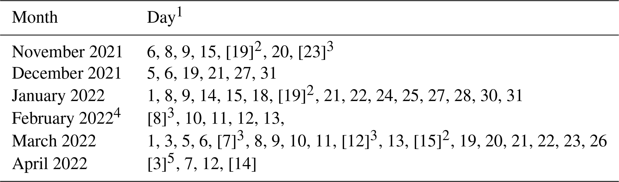
¹ Brackets [ ] indicate that the local-arc breaking was seen in the image without a Level 6 alert. ² Moon contamination prevented the identification of the “strong aurora” category, with L3 = 0 for 19 November, L3 = 6.9 for 19 January, and L3 = 7.8 for 15 March. ³ local-arc breaking in the northern sky only such that the numbers of strong aurora pixels did not reach the criterion. ⁴ The ASC did not operate on 16–19 and 21 February (a total of five nights). ⁵ Relatively weak local-arc breaking in the dusky sky with some sunlight effect remaining such that the exposure time is too short to recognize sufficient numbers of aurora pixels.

Unless the aurora brightening takes place very far north, above the cloud, or hidden by the Moon, the eye-identified aurora brightening is well represented by Level 6 within 10 min. Here, most of the false negatives (detection of Level 6 without a local-arc breaking within 10 min) were issued during the intensification of the auroral arcs before the local-arc breaking or during the expanded auroral activity like a substorm expansion phase (Akasofu, 1977) and are related to the same series of aurora activity related to the local-arc breaking. Only a small fraction of such false negatives was un-associated with a substantial expansion of the aurora (about 10 %).

Likewise, the present method gave a small percentage of false positives: the Level 6 auroral activity was not detected 9 nights out of nearly 50 nights with the local-arc breaking in the ASC. After removing the local-arc breakings that are affected by Moon or twilight, this ratio decreases to 4 nights out of about 45 nights. Even if we count the individual local-arc breaking when multiple events take place in one night, this low false rate does not change very much. Thus, after 5 months' operation, the Level 6 definition in the present version (version 1.0) works properly in identifying the local-arc breaking for both the real-time campaign and statistical studies.

4 Examples

In this section we show examples of the ASC auroral index and ASC images around the local-arc breaking.

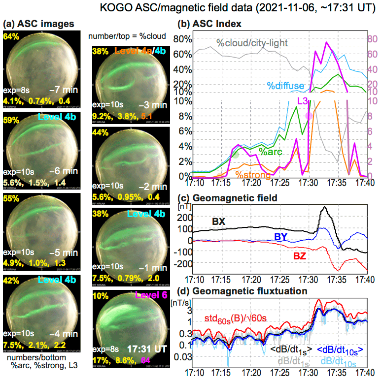
Figure 7 ASC and magnetometer data around 17:31 UT on 6 November 2021: (a) aurora images (the same coordinates as in Fig. 2); (b) ASC auroral index values; (c) DC geomagnetic deviation from the baseline values (X = north, Y = east, Z = downward); and (d) AC geomagnetic variation $\mathrm{|}\mathrm{d}B/\mathrm{d}t\mathrm{|}$ measured by three different methods. In each image in (a), the ASC auroral index values of %arc, %strong, and L3 are given at the bottom, above which the automatic exposure time and UT are given. The cloud coverage (%cloud) and the activity level (Level 6, Level 4a, and Level 4b) are given at the top. The timing of Level 6 detection is the same as the onset of the local-arc breaking. In the auroral index panel (b), the scaling is changed for below 10 and above 10 (therefore the graph has a gap in between). The three methods of $\mathrm{|}\mathrm{d}B/\mathrm{d}t\mathrm{|}$ in (d) are (1) using 1 s values (black), (2) using 10 s running average values (blue), and (3) the standard deviation of magnetic field over 60 s, using 1 s values and normalized to nT s⁻¹ unit (red). These variations are first calculated for each vector component and then for the absolute values.

4.1 Successful cases

The first Level 6 activity after we started the automated email alert was detected on 6 November 2021, a day after we started the system (it was cloudy on 5 November). Figure 7a shows the series of Kiruna ASC images around the first Level 6 detection on that day. The ASC auroral index values are given at the bottom of each image. In addition, cloud coverage (in %) is given at the top of each image in Fig. 7a (but not in the other figures with ASC images). The automatic exposure time (8–10 s) is much longer than those in Figs. 1, 2, 4, and 6 (1–5 s), partly due to the non-Moon conditions (this is why the city light is bright compared to previous images). Each image is taken toward the sky with north at the top, and hence east (west) is on the left (right).

In Fig. 7a, the local-arc breaking (most likely the arrival of the auroral substorm bulge at this local time) is seen at 17:31 UT (around 20 MLT) and simultaneously Level 6 is detected, both happening for the first time, on this evening. Before this local-arc breaking, the intensification of the auroral arc equatorward of the original arc was recognized at 17:27 UT (4 min before). In this example, two of three Level 6 conditions (%arc ≥ 3 % and %strong ≥ 0.2 %) are satisfied already at 17:18 UT, as shown in Fig. 7b, and L3 ≥ 8 is the condition that demarcates the activity level.

As a reference, we also show the geomagnetic variation during this period in Fig. 7c and d. Figure 7c shows fluxgate (DC) magnetometer data B, and Fig. 7d shows its variation $\mathrm{|}\mathrm{d}B/\mathrm{d}t\mathrm{|}$ that is represented by three different methods: simple $\mathrm{|}\mathrm{d}/\mathrm{d}t\mathrm{|}$ values using 1 s resolution data and a 10 s running average (still 1 s resolution) data and the standard deviation divided by the square root of 60 s (∼7.75 s^0.5), i.e., the normalized fluctuation over 60 s. At 17:31 UT when the aurora brightening reached Level 6, the geomagnetic field suddenly changed, with B_X starting to change by more than 100 nT within 1 min (this satisfies necessary condition of a substorm), while the magnetic deviation increased by an order of magnitude in all three methods.

The next detection of Level 6 activity was under more cloudy conditions at 20:43 UT (around 23 MLT) on the same day. Figure 8 shows the series of Kiruna ASC images, time series plots of the ASC auroral index values, and geomagnetic activities in the same format as in Fig. 7 except that the cloud coverage is not given in the ASC images. The automatic exposure time (8 and 5 s) is the same as or slightly shorter than those in Fig. 7. Due to heavy cloud coverage (almost full coverage over the sky), the auroral arc was not well recognized until 1 min before the local-arc breaking (20:42 UT), at which only one parameter (%arc) reached the criterion of Level 6, while the other parameters (%strong and L3) did not reach the criterion of Level 4a or b. Fortunately the cloud was not very thick and the brightening of the aurora was strong enough to be recognized in the ASC auroral index. The timing of Level 6 detection (20:43 UT) again corresponds to a large geomagnetic deviation with a change greater than 100 nT in B_X and a nearly 1 order of magnitude increase in the magnetic deviation in all three methods.

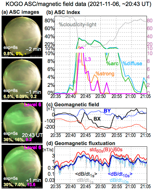
Figure 8 The ASC images, ASC auroral index values, and geomagnetic data from around the time when the Level 6 auroral activity was detected at 20:43 UT on the same night as in Fig. 7. The format is the same as in Fig. 7 except that the cloud coverage is not shown in the ASC images.

In both examples (17:31 and 20:43 UT), Level 6 detection timing agrees with the timing of the local-arc breaking in the ASC image, and the morphology of the local-arc breaking is consistent with the evening aurora surge during a substorm (Akasofu, 1964). The last detection of the Level 6 activity on the same night at 23:15 UT took place in the post-midnight sector (around 01 MLT). Figure 9 shows the relevant images and plots in the same format as in Fig. 8. The automatic exposure time (8–10 s) is the same as those in Fig. 7. In this example, the aurora brightening started already at 23:13 UT, 2 min before the Level 6 detection, as is also indicated by the geomagnetic deviation (90 nT change in the X component in 2 min). Instead of Level 6, ASC auroral index values gave Level 4b at 23:13 UT and Level 4a at 23:14 UT (%arc = 8.2 %; %strong = 0.25 %; and L3 = 6.1). The magnetic deviation also increased significantly, but the peak values are much lower (by more than a factor of 3) than previous Level 6 activities (Figs. 7 and 8). Considering such small geomagnetic activity and its post-midnight location, the 2 min delay of Level 6 detection is still successful for the real-time alert.

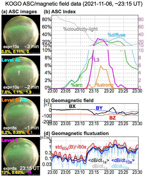
Figure 9 The same as Fig. 8 for the Level 6 auroral activity at 23:15 UT on the same night as in Figs. 7 and 8.

Since the morphology and intensity of the aurora are quite different in the pre-midnight and post-midnight sectors (e.g., Akasofu, 1964), the relation between the ASC auroral index and the aurora intensification must also be different between them. For example, the diffuse aurora in the post-midnight sector is often registered in the green arc category because of its high intensity. Ideally, different criteria should be used for pre-midnight and post-midnight sectors. On the other hand, the present algorithm detects Level 6 for many of post-midnight cases anyway because the criterion of the L3 value is not affected very much. This is why we keep the consideration of the local time as a future task but not very urgent.

4.2 Moon effect

Here, we show two examples strongly influenced by the Moon: one successful case (15 November 2021, 20:36 UT) in Fig. 10 and one unsuccessful case (19 January 2022, 23:57 UT) in Fig. 11. The examples with the Moon in Figs. 1, 2a, and Fig. 6 (20:50 and 23:02 UT) also satisfy the Level 6 criterion. In Fig. 10, Level 6 was detected at 20:36 UT, which is only 2 min after a signature of the local-arc breaking becomes visible in the ASC. The automatic exposure time (4 s) is the same as that in Fig. 2a and similar to those in Fig. 6c, both with the Moon. For this event, the brightened aurora is located very close to the Moon, and that caused relatively low L3 values and low %strong values. Nevertheless, the values of the ASC auroral index reached Level 6. Compared to the local magnetometer data (Fig. 10c and d) that indicate the local-arc breaking at 20:39 UT, the ASC auroral index gave a closer time to the local-arc breaking.

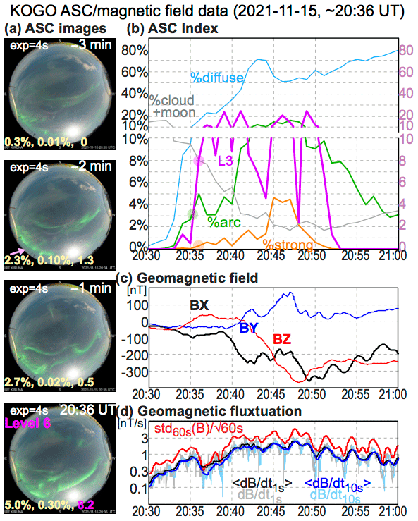
Figure 10 The same as Fig. 8 for the Level 6 auroral activity at 20:36 UT on 15 November 2021.

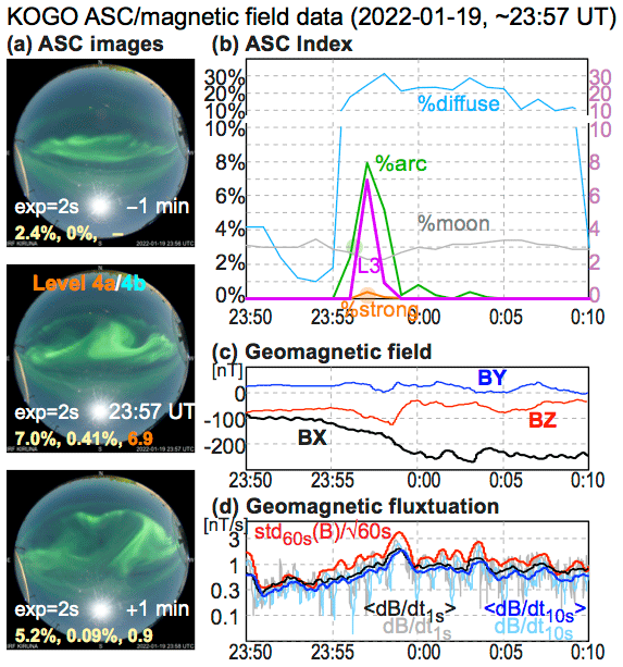
Figure 11 The same as Fig. 8 for the Level 4a/b auroral activity at 23:57 UT on 19 January 2022.

In the unsuccessful case (Fig. 11), the peak L3 value was only 6.9 at 23:57 UT, although the ASC image shows the local-arc breaking some distance north of the Moon. The automatic exposure is shortened to 2 s, the same as the cases with the Moon in Figs. 1a and 2b. Both the geomagnetic deviation (>150 nT within 5 min) and the magnetic variation reaching nearly 3 nT s⁻¹ 1 min after at 23:58 UT (same level as in Figs. 7, 8, and 10) indicates that auroral activity corresponds to the local-arc breaking. With %arc = 7.0 % and %strong = 0.41 % at this time, only the L3 value did not reach the Level 6 criterion.

The small L3 value must be mainly due to reduced exposure time by the existence of the Moon but might also come from wide refraction of moonlight through the dome that also changes the color (H value) of the aurora pixels. As a result, even the color in background pixels (night sky) becomes more bluish than the case on 6 November 2021. We consider the color shift important because the next example (Fig. 12) with longer exposure time is also unsuccessful. Taking care of these problems is one of the future tasks.

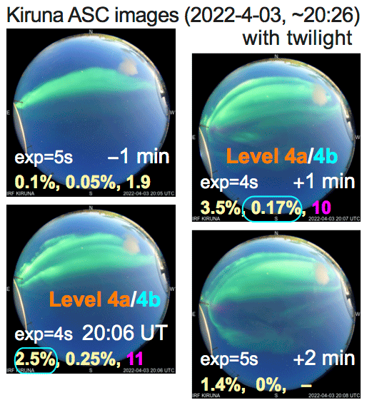
Figure 12 ASC images around 20:06 UT on 3 April 2022, when the ASC auroral index values did not reach Level 6 due to the twilight effect when the local-arc breaking took place.

4.3 Twilight effect in spring and fall

Like the Moon effect case, twilights also change the color of the entire image toward blue. Figure 12 shows one such unsuccessful case. The automatic exposure time (4–5 s) is similar to the exposure time in the successful Moon cases (Figs. 6 and 10). A clear local-arc breaking took place in the northern sky. In fact the L3 value exceeded the Level 6 criterion at 20:06 and 20:07 UT. However, the aurora coverage (either %arc or %strong) did not reach the values needed (marked by a blue circle in the figure). Thus, the short exposure time alone does not prevent the ASC auroral index reaching Level 6.

4.4 Missed case due to northward aurora location

If the local-arc breaking takes place in the northern sky with a large zenith angle, the geometric effect (see Sect. 3.4) reduces the aurora coverage (%arc and %strong). This sometimes prevents the detection of local-arc breaking, particularly for relatively weak ones. Figure 13 shows one such example of the local-arc breaking in the far northern part of the field of view (23 November 2021, 21:28 UT) without reaching Level 6 due to too small aurora coverage. The automatic exposure time (3–4 s) is within the range of the successful cases shown in Figs. 1, 10, and 11, thanks to a thin cloud reducing the Moon effect. The brightest image was taken at 21:29 UT with sufficient %strong pixels (= 1.15 %) and L3 (= 9.5) for Level 6, but %arc (= 1.9 %) was far below the required threshold (≥ 3 %) for Level 6 (marked by a blue circle in Fig. 13a). The geomagnetic deviation (Fig. 13c) of more than 100 nT and geomagnetic variation (Fig. 13d) of about 1–3 nT s⁻¹ are large enough to be accompanied by a local-arc breaking, considering the location of the aurora far north that causes reduced geomagnetic signatures.

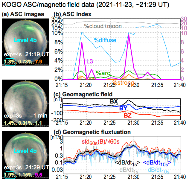
Figure 13 The same as Fig. 8 for the Level 4b auroral activity in the north at 21:29 UT on 23 November 2021.

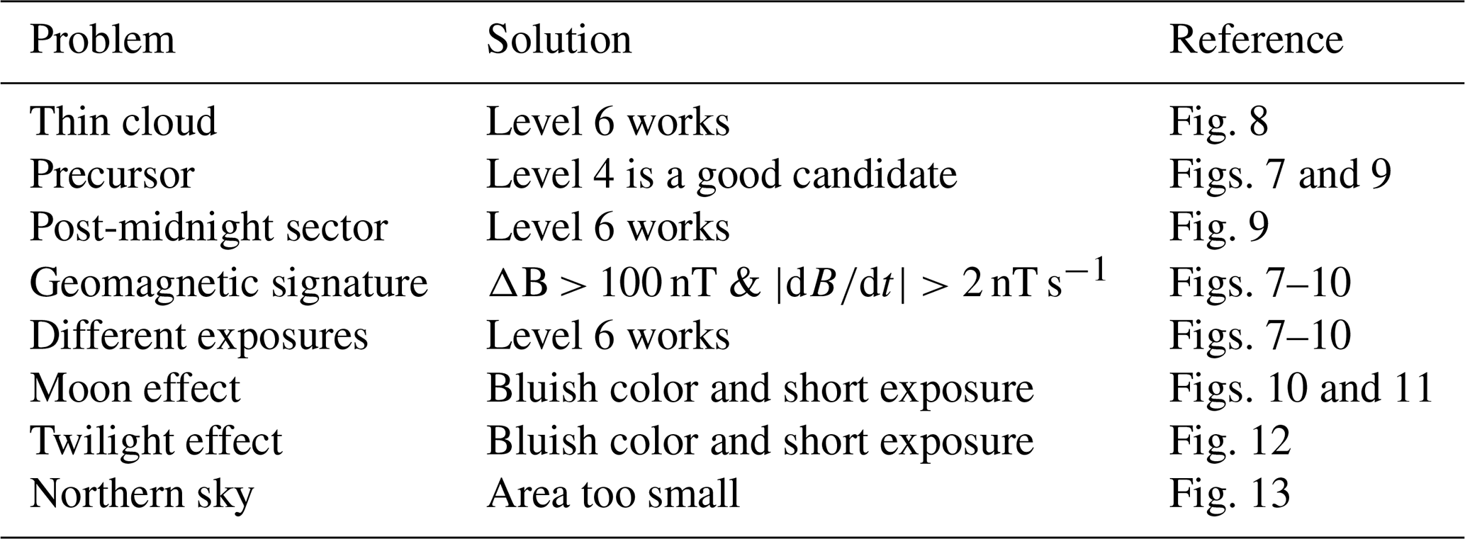
Table 8 summarizes the features and problems that are explained in the examples in Figs. 7–13.

Table 8 Summary of examples.

5 Discussion

We used three categories of aurora instead of two (discrete aurora and diffuse aurora) in Sect. 3.2. Adding a third fuzzy category between two different phenomena is a common practical method in classifying data, and this method is particularly useful here because our aim is to identify the intensification of the aurora rather than the aurora itself. For the same reason, one may add a new category of “potential aurora” that does not reach the criterion of visible diffuse if the purpose is just to identify images that may contain visible aurora, for example, for automatically removing the ASC image from the archive (with the condition of no aurora and high cloud coverage).

The present scheme is the first automated quantification scheme of real-time auroral activity level, particularly the local-arc breaking (it is actually in operation even in the 2022/2023 season). It is also the first trial of numerical translation regarding how aurora scientists judge the auroral activity (e.g., Akasofu, 1977). Such a quantification ability is the main difference to existing machine-learning schemes (e.g., Nanjo et al., 2022, and references therein): none of them has yet quantified the auroral activity (neither corresponding to the ASC auroral index or the activity level).

Several groups have started the identification (even classification) of the aurora using machine-learning methods (eventually deep learning neural networks) directly from ASC images in the RGB color code (e.g., Clausen and Nickisch, 2018; Kvanmmen et al., 2020; Nanjo et al., 2022, and references therein), and even the real-time classification is implemented (Nanjo et al., 2022) (https://tromsoe-ai.cei.uec.ac.jp/, last access: 11 April 2023). However, what so far exists is only classifying the entire sky into different categories, using a training set. For example, Nanjo et al. (2022, Fig. 1) and their reference (Clausen and Nickisch, 2018, Fig. 1) have three aurora categories (“arc”, “discrete”, “diffuse”), as one value for each image (here “arc” is scientifically just a special form of “discrete”), but “discrete aurora” and “diffuse aurora” always appears together during or just before high auroral activity. Also, no machine-learning method has quantified the intensification of the discrete (arc) aurora (at least the current authors are not aware of this), although such a quantification is inevitable in judging the local-arc breaking. Since most of the aurora images are mixed with clouds (it is very rare to have a clear sky for an entire night), the classification of the entire image as one category may often end up being “ambiguous” (Clausen and Nickisch, 2018) or “aurora and cloud” (Nanjo et al., 2022).

Another advantage of using the two-step expert system (sets of solid criteria) is that it is relatively easy (for aurora scientists) to pinpoint the reason for any judging error. For example, a masking matrix of $\sim \mathrm{1.4}\times {\mathrm{10}}^{\mathrm{5}}$ pixels with true and false values for each category is also stored as a mid-term product for each category before deriving the ASC auroral index. This allows a pixel-level examination (see Fig. 1c–e) in the case of categorization errors. This method is actually used to separate the cloud effect during the development of the criteria (Tables 2 and 3). We have also identified the reason for the false positive for the Moon cases: it is due to the color shift in all pixels toward blue by the refraction of the moonlight through the all-sky dome.

On the other hand, the machine-learning methods may improve or simplify the present method by applying the machine-learning methods to each step (step 1a and step 2), while the logic and aim for each step are kept the same. For example, step 1 may be improved by using the random-forest method (Breiman, 2001; Liu et al., 2017) in addition to deep learning. Likewise, the machine-learning method may help improve step 2 only. Conversely, by comparing with the outputs of the present method, improvement in the machine-learning scheme may also become relatively easy.

As a final note, we do not have to change the entire logic but only to adjust the criteria for different ASCs at different locations, although the present criteria are specific to the Kiruna ASC. If the camera and settings are the same, even the present criteria may well be used for the other location. This is because the RGB color area (particularly the $\mathrm{R}/\mathrm{G}$ ratio for different G ranges) of the non-aurora sources does not overlap with those of the strong aurora or green arc (the present version 1.0 uses only these two categories for activity evaluation). For example, relatively simple cloud identification by the sodium line for Kiruna (589 nm, due to the strong light pollution by the city), which sometimes has similar hue (H) values to the weak aurora, does not alter the identification of the local-arc breaking very much. Also, a difference in the auroral morphology at different latitudes does not alter the identification of the local-arc breaking itself very much. At low-latitude stations where the local-arc breaking occurs at the northward edge, the activity is underestimated due to geometric effects, but the activity in the middle of the sky is still correctly estimated.

For different camera manufacturers/models that have different color characteristics, we just need to make different criteria, but the general color range must be similar to the present ones. Then, we can aim to obtain the similar ASC auroral index values for the same level of activity between different ASC stations.

6 Summary and conclusion

We developed an automatic identification scheme for the sudden and significant intensification of the auroral arc with expanding motion (local-arc breaking) seen in the ASC JPEG image that is recorded in the RGB color code and applied it to create a real-time alert. Unlike the other automatic identification trials, such as using a deep-learning neural network (none of them has so far quantified auroral activity), we used a set of simple criteria and calculations (expert system). The scheme is divided into two steps:

1. A set of simple numbers, the ASC auroral index, is defined such that it represents the sky condition of the entire ASC ($\sim \mathrm{1.4}\times {\mathrm{10}}^{\mathrm{5}}$ active pixels with 3-byte color information each).

2. The auroral activity level is judged only from the index values. The mid-term product (ASC auroral index) is stored on a real-time basis, whereas the result of activity assessment is sent as a warning real-time email when the index values satisfy the Level 6 criterion.

The first step is further subdivided into two stages: (1a) pixel-to-pixel classification into strong aurora, most likely auroral arc (category green arc), most likely visible diffuse aurora (category visible diffuse), most likely the cloud category, most likely the Moon category, and most likely the artificial light category, using just R, G, B, and hue (H) values (where H is calculated from the RGB values); (1b) a simple calculation such as the percentage of the occupying area (pixel coverage) and the characteristic intensity of the strong aurora (taking the nonlinear average of luminosity L and L³ for the most luminous 4900 pixels).

After 5 months of the operation until the end of the 2021/2022 winter season, this algorithm successfully issued an alert for the local-arc breaking within 10 min of when the actual brightening of the aurora is detected for nearly 90 % of cases (see Table 7). Likewise, the percentage of false negatives was also low.

The present scheme is only version 1.0, and there is considerable room for improvements. Its direction is clear, thanks to the present method with the explicit criteria and calculations: we need to upgrade the criteria at each step, based on further understanding of, for example, the camera characteristics regarding different light sources and their relation to the geomagnetic activities (see Appendix B for these tasks).

Appendix A: Version 0 classification using only HSL values

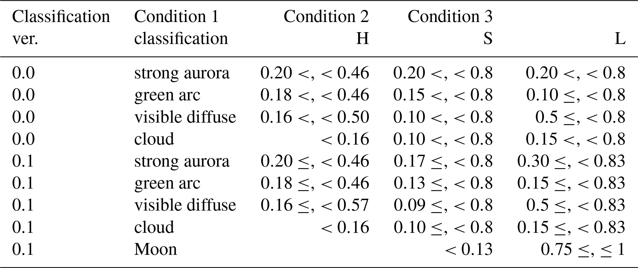
For the old KAGO's ASC (Nikon D700 camera) until April 2020, we used a less accurate classification method using HSL values only to obtain the ASC auroral index version 0 (Yamauchi et al., 2018). In this version, we just plotted the index values on our website on a real-time basis, and its archive is found at the IRF site (https://www.irf.se/maggraphs/aurora_detect/graphs/, last access: 11 April 2023). For this real-time operation, we used the criteria (version 0.0) that are summarized in Table A1.

This version (version 0.0) was slightly updated for the data analysis when the operation of the old ASC (Nikon D700 camera) ended. The revised criteria (version 0.1) are summarized in the same table (Table A1).

Table A1 Version 0.0 criteria of the ASC auroral index for the old ASC (Nikon D700).

Appendix B: Future improvements

In Appendix B, we list tasks for future improvement that we consider feasible, in addition to tuning the criterion values (e.g., 2.8 % instead of 3.0 % for %arc in the Level 6 criterion).

These improvements require further subdivision of the aurora image (e.g., different local times, different exposures, different aurora with Moon) and, hence, require more aurora examples to examine than what we have examined so far.

B1 Correction using exposure time information (for step 1) and UT information (for both steps)

The present version is made to judge only from the JPEG image but not using hidden information. This is because the analysis code (see Supplement) can be easily modified for the other ASC images, e.g., taken at non-scientific stations (Toyomasu et al., 2008). However, we can use two extra pieces of information that are available in most JPEG images. One is the UT information that is tagged to the ASC images in most cases. The other is the exposure time given as hidden information for the JPEG file (can be extracted with, e.g., the “exiftool” command, for the Python programming language). Although the present version identifies most of the local-arc breaking for different UTs and for different exposure times, including these pieces of information will further improve both the ASC auroral index and activity level definition. For example, we can treat the post-midnight diffuse aurora during a substorm separately because it is often too strong and often misjudged as the auroral arc (green arc category).

B2 N₂ red (670 nm) line (for step 1)

In the present version, all aurora pixels must satisfy R < G and B < G (the same as 0.167 ≤ H < 0.5) to avoid any contamination from white light or twilight. This automatically removes the strong red emission by N₂ around 670 nm (mainly <100 km altitudes) shown in Fig. 4b or the faint blue emission by ${\mathrm{N}}_{\mathrm{2}}^{+}$ at 428 nm (mainly >150 km altitude). Adding these lines, particularly the strong N₂ red line, would improve the strong aurora definition. Fortunately, the N₂ red line in Fig. 4b does not belong to any category yet, opening up the possibility of adding a new category, “N₂ aurora”. To add this category, we must examine more examples with strong N₂ red lines (they are rare) to find out the relevant RGB color code, while limiting ourselves to the RGB color range different from twilight, the Moon, and other light sources. The priority is lower for extracting the ${\mathrm{N}}_{\mathrm{2}}^{+}$ blue line than the N₂ red line because the ${\mathrm{N}}_{\mathrm{2}}^{+}$ blue line appears more often near the equinoxes than in winter, and including the ${\mathrm{N}}_{\mathrm{2}}^{+}$ blue line may cause inequality between different seasons.

B3 Moon filter and twilight filter (for step 1)

To reduce the Moon effect, we currently mask all pixels within a radius that is 14 times the detected Moon radius (even the radius of the Moon changes with time, location, and Moon phase) because both the sky and the all-sky dome scatter the moonlight, modifying the color and intensity of the aurora pixels in a wide area around the Moon during almost all Moon phases. Of course the Moon itself blocks the aurora in its vicinity.

Just masking the Moon from date and time is not practical because the all-sky dome modifies the Moon location and size. Also, the effect (shift in the color toward blue) is seen in almost all pixels in the entire image, with a higher effect closer to the Moon. One possible counterpart is to use “corrected B” values that are reduced from the obtained B values, depending on the distance from the Moon. The goal is to make similar values of the ASC auroral index (for strong aurora and green arc, at moment) for the same level of the aurora activities with and without the Moon. We can make a similar correction for twilight, but this is not as urgent as the Moon correction because the twilight problem is seen only at the beginning and end of the season when the night is very short.

B4 Defining less intense but sudden intensification as Level 5 (for step 2)

Some local-arc breakings are more compact and less intense than others. Some of them are even difficult to distinguish from simple intensification or deformation of auroral arcs, e.g., a real expansion of the bright regions or some brightening that soon returns to the green arc again without expansion. Therefore, it would be useful to have a category of minor sudden intensification, such as Level 5. Such an introduction of “fuzziness” makes the alert system more reliable.

B5 Dividing the field of view (for both steps)

The present ASC auroral index treats all pixels equally, which gives the zenith aurora more weight in the calculation of the index values than the other parts of the sky due to the physical geometrical effect, while another type of weighting is introduced by the fish-eye lens's optical geometry. Furthermore, the local-arc breaking in the southern sky expands toward the entire sky (Akasofu, 1977), giving higher index values than the local-arc breaking in the northern sky, which expands mainly toward the northern edge. These “aurora location” problems (reliable only near the zenith or slightly south of it) should ideally be solved by placing many ASCs with 100 km's distance from each other. Meanwhile, we can make some improvement with a single ASC by dividing the field of view into two-three areas (north, middle, south) and obtaining the index values for each area, in addition to introducing simple correction that depends on the zenith angle. When calculating the final index values, we can weigh differently between these three regions (more weight for the northern sky than southern sky).

B6 Previous 5 min activities (for step 2)

For some local-arc breaking cases without the Level 6 alert, its criterion is satisfied if we take peak values of the ASC auroral index within 5 min (four cases in 2022 out of eight nights in Table 7: 8 February, 7 March, 12 March, and 3 April). These examples suggest the possibility of loosening the criterion by using nearby data (timing). Another possible solution is to introduce gradients of values such as sharp increases in %strong and L3 as the condition for easing the criterion. Such attempts are also useful in defining Level 5 (less intense aurora intensification) and lower levels of activity. The problem is that the optimization requires complicated examinations of multi-minute data, and finding the solution is not simple. This could be a good task for the machine-learning methods.

B7 Precursor or Level 4 (for step 2)

As an extension of the previous task (considering previous 5 min activity), we can even search for precursor signatures of the local-arc breaking. Level 4a and Level 4b are defined as the first step for this effort, and the methods mentioned above (including machine-learning methods) will help tune Level 4. If using the machine-learning method, only the ASC auroral index values during the past 10 min should be used to predict Level 6 activity without examining the image data. Then, the ASC auroral index values between 5 min before Level 6 and 10 min before Level 6 can be good reference values in defining Level 4.

B8 Adding geomagnetic variation (for both steps)

As an external index, local geomagnetic activity can be used to help define the level (e.g., Juusola et al., 2020). To evaluate the optimum information for this purpose, we showed geomagnetic variations in Figs. 7–11 and 13 in both DC and AC formats. As the AC variation, we showed $\mathrm{|}\mathrm{d}B/\mathrm{d}t\mathrm{|}$ values obtained from the 1 s resolution values and from 10 s resolution values and their 1 min running averages. We also showed the theoretical accuracy of the 1 s resolution values, i.e., the standard deviation divided by the square root of 60 s, giving the result with the same unit [nT s⁻¹] as other parameters.

A change in B_X (deviation within 10 min or so) is the optimum parameter for DC variation, whereas all AC profiles are similar to each other, suggesting that using 10 s values is sufficient as the source data when 1 s resolution data are not available. On the other hand, the standard deviation method might be optimal if the computation time is short enough. This problem is directly related to the geomagnetically induced currents (GICs) during the space weather hazard events. This means that we can even search for possible precursors of the big GIC events (big $\mathrm{|}\mathrm{d}B/\mathrm{d}t\mathrm{|}$ events) in the ASC auroral index.