Macapá, a Brazilian equatorial magnetometer station: installation, data availability, and methods for temperature correction

In the last 60 years, the largest displacement of the magnetic equator (by about 1100 km northwards) occurred in the Brazilian longitudinal sector. The magnetic equator passed by Tatuoca magnetic observatory (TTB) in northern Brazil in 2012 and continues to move northward. Due to the horizontal geomagnetic field geometry at the magnetic equator, enhanced electric currents in the ionosphere are produced – the so-called equatorial electrojet (EEJ). The magnetic effect of the EEJ is observed in the range of ±3° from the magnetic equator, where magnetic observatories record an amplified daily variation of the H component. In order to track the spatial and temporal variation of this phenomena, a new magnetometer station was installed in Macapá (MAA), which is about 350 km northwest of TTB. In this paper, we present the setup and data analysis of MAA station from November 2019 until September 2021. Because of its special configuration, we develop a method for temperature correction of the vector magnetometer data.

1 Introduction

With globally distributed geomagnetic observations it is possible to investigate the different geomagnetic field sources in the core (the largest part of the measured field), crust, ionosphere, magnetosphere, and induced fields (Hulot et al., 2010). Temporal variations in the Earth's magnetic field at ground level are monitored by geomagnetic observatories (Matzka et al., 2010) and magnetometer stations (Chulliat et al., 2017). Dedicated geomagnetic satellite missions provide observations from low Earth orbit. Magnetic observatories produce high-quality and continuous data over long periods (Matzka et al., 2010). Precise and frequent absolute measurements of declination and inclination by trained staff are required to calibrate geomagnetic observatory data. Observatories belonging to INTERMAGNET (International Real-time Magnetic Observatory Network) follow quality standards for measuring and transmitting real-time data (St-Louis et al., 2020). They are an important data source for studies of the internal geomagnetic field and its secular variation and studies of space climate, e.g. with the help of geomagnetic indices. However, there is an uneven spatial distribution of magnetic observatories around the globe, which is worse in the Southern Hemisphere and oceans. There are many reasons for such uneven distribution, such as infrastructure requirements, data transmission problems (especially in remote areas), need for trained staff, and a lack of investments that are fundamental to maintain or construct new observatories. On the other hand, magnetometer stations are not so demanding in terms of infrastructure and staffing requirements. The three components of the magnetic field are measured continuously in a magnetometer station, as is done in the observatories; however, absolute measurements are not periodically acquired. Typically, magnetometer stations are intended to monitor the external and induced geomagnetic fields. They can also be used as a first step to investigate the suitability of a new location before constructing a geomagnetic observatory.

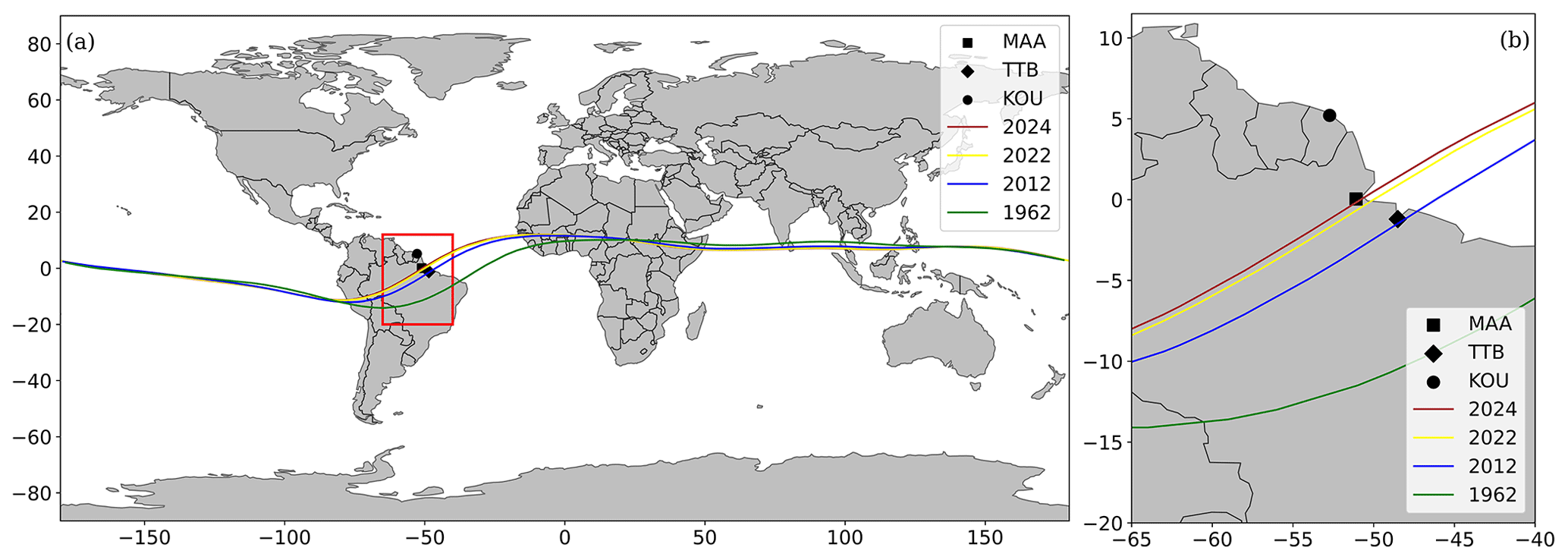
Figure 1 Magnetic equator calculated by the IGRF-13 (a) for 1 July of the following years: 1962 (green line), 2012 (blue line), 2022 (yellow line), and 2024 (red line). The zero-inclination lines are calculated considering 105 km altitude, the region where the equatorial electrojet is produced. In (b) a zoomed-in view of South America is shown, with the locations of Tatuoca (diamond), Kourou (circle), and Macapá indicated (square).

In Brazil, there are two INTERMAGNET observatories: one in Vassouras (VSS – Rio de Janeiro, RJ) and another in Tatuoca (TTB – island in Belém, PA), which have continuously measured the magnetic field since 1915 and 1957, respectively. There are two important magnetic phenomena in Brazil: the South Atlantic Anomaly (SAA), where the magnetic field intensity is the smallest globally, and the magnetic equator, where the magnetic inclination is zero.

In the last 60 years, the displacement of the magnetic equator in Brazil was the largest in the entire globe: 1100 km northwards, as predicted by the IGRF-13 (International Geomagnetic Reference Field) model (Alken et al., 2021). In Fig. 1 the magnetic equator is shown for different epochs in the last 60 years along with the forecast for 2024, where the secular variation of the inclination predicts the largest changes over Brazil (Alken et al., 2021). In this zero-inclination region, the magnetic field is mostly horizontal, and as a consequence strong ionospheric electric currents at about 105 km altitude are produced on the day side. These currents extend to about ±3° from the magnetic equator and are known as the equatorial electrojet (EEJ), as reviewed in Yamazaki and Maute (2017). The result is an intensification of the H-component daily variation (Soares et al., 2020), reaching up to about a 100 nT (see example in Fig. 2). In 2012, the magnetic equator passed over TTB, and its amplified diurnal variation was analysed by Soares et al. (2020). When compared to fields generated by solar quiet currents (Sq) from low and medium latitudes, the magnetic field in TTB shows a special variation influenced by the seasons, atmospheric oscillations, and lunar tides.

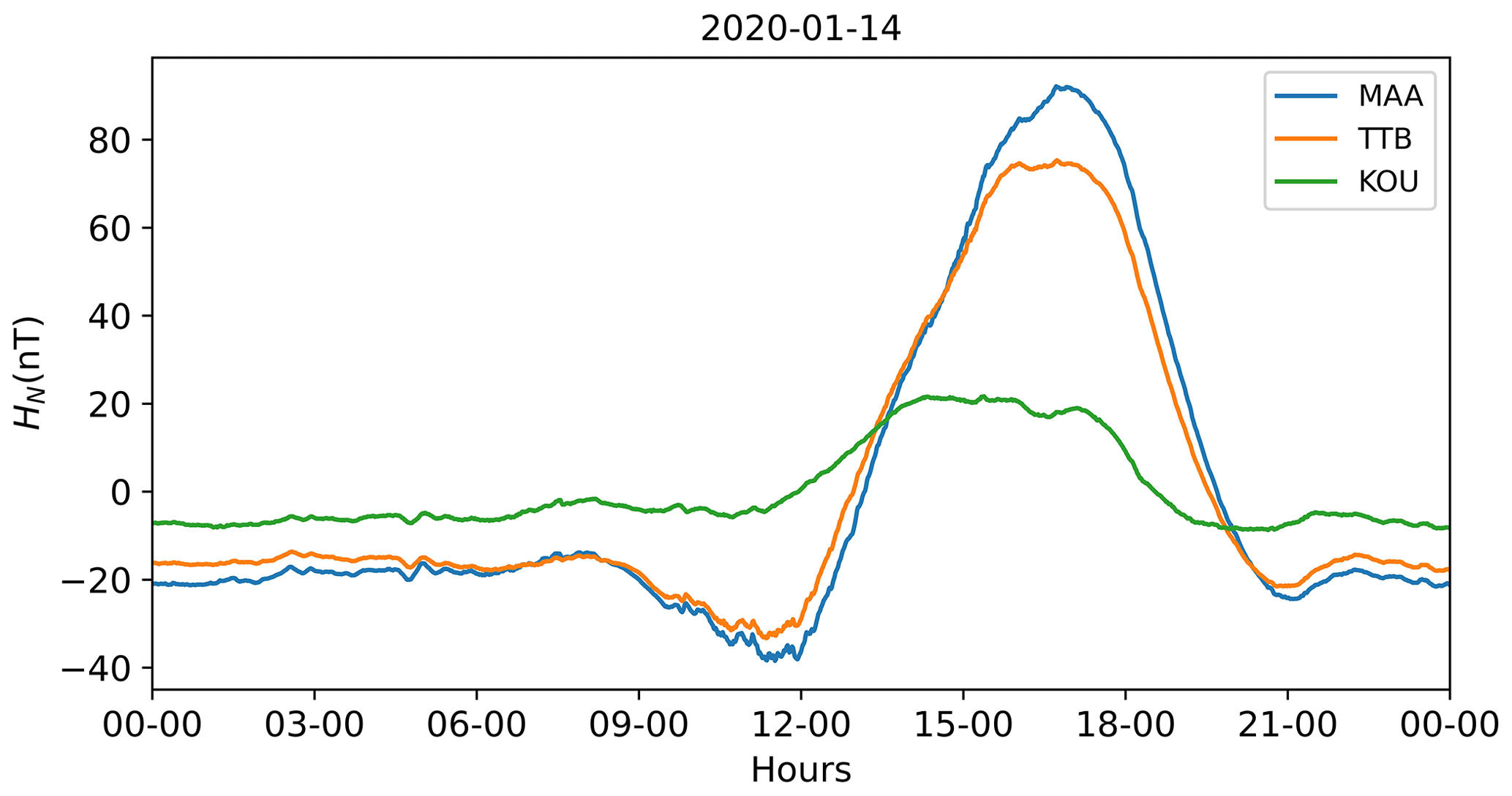
Figure 2 Comparison between the north-component daily variation of Tatuoca (TTB, 1.20° S, 48.51° W) and Kourou (KOU, 5.21° N, 52.73° W) magnetic observatories and the north component in the sensor coordinate system (H_N) of Macapá station on 14 January 2020. Local noon at TTB is 15:00 UTC.

The magnetic equator continues to move northwards, and it is predicted by the IGRF-13 model (Alken et al., 2021) to be located at Macapá station at around July 2024 at Macapá station altitude (see Fig. 1). Therefore, a new magnetometer station was installed in Macapá in order to track the effects of the equatorial electrojet. This work is a result of a cooperation between Observatório Nacional (Rio de Janeiro, Brazil), Universidade Federal do Pará (UFPA, Brazil), and GFZ Potsdam (GFZ, German Research Center for Geosciences).

In order to choose the best location for Macapá station, two sites were tested in May 2019, i.e. at Chaves (0.180° N, 49.954° W, 2 m altitude) and at IEPA (Institute for Scientific and Technological Research of the State of Amapá, 0.038° S, 51.095° W, 34 m altitude). The total magnetic field was measured at both locations and 50 m to the north, south, east, and west of it. Since only a weak magnetic gradient of around 1 nT was found, the total field was measured for 3 consecutive days in both locations in order to check the data quality and possible noise from environmental interference. Both locations showed good data quality and good agreement with simultaneous TTB data. The access to Chaves is more difficult due to an 8 h trip by boat, while IEPA is more accessible. In addition, since IEPA is a public institution, local staff and infrastructure are available, which are both fundamental for the success of magnetometer stations in remote areas. Fluxgate magnetometers for measuring the components of the geomagnetic field are temperature sensitive, and magnetometer stations typically do not have a temperature-controlled environment. Several methods have been used and published to first determine temperature coefficients of such magnetometers and then correct the recorded raw data (e.g. Janošek et al., 2018; Kudin et al., 2023).

2 Macapá station setup

In November 2019 the magnetometer station of Macapá (MAA) was installed on the IEPA campus (Fig. 3). There is no unique technique to install a magnetometer station since each location has its own requirements depending on the local conditions like weather, infrastructure, and staff availability. Two instruments measuring the magnetic field were installed in Macapá. A triaxial fluxgate magnetometer (GEOMAG-02 by Research Centre GEOMAGNET) measures the horizontal north (H_N), horizontal east (H_E), and vertical (Z) components (Appendix A) in the orthogonal sensor coordinate system. During the installation of the GEOMAG sensor set, we aligned it in a way that H_E is zero. The sampling rate is 1 Hz, and the time stamping is controlled by GPS and Network Time Protocol (NTP). The second instrument is a scalar Overhauser magnetometer (GSM-90 Overhauser by GEM Systems), which measures the scalar field strength F. The sampling rate is one sample every 5 s and NTP is used for the time stamping.

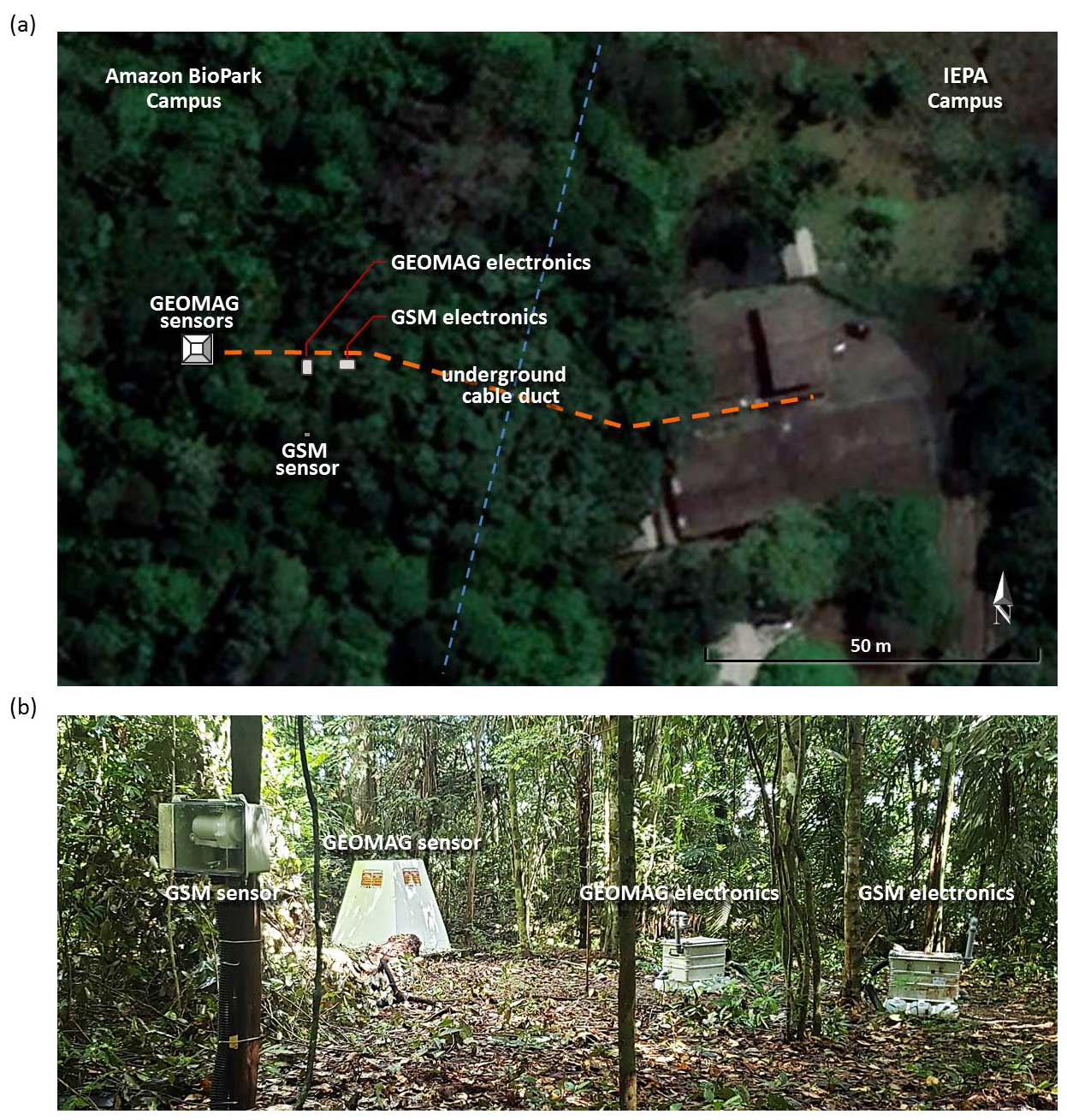
Figure 3 (a) Location of Macapá station (IEPA campus) showing the locations of the sensors and electronics. (b) An image of the fibreglass pyramid and the boxes with GEOMAG and GSM electronics.

The GEOMAG sensor is installed inside a fibreglass shelter for protection against rain and wind (Fig. 3). This shelter has thermal insulation and is pyramid shaped (with a flat top; see Fig. 4), as was done for Tristan da Cunha observatory (Matzka et al., 2011). This design is similar but lighter than the pyramid described in Matzka et al. (2011). The foundation of the pyramid is made of concrete about 25 cm thick and 70 cm deep. The instrument pillar is also made out of concrete. It is completely separate from the pyramid foundation, about 60 cm × 60 cm in cross section, 70 cm deep, and extends about 30 cm a.g.l. (above ground level). The fluxgate sensor is located directly on the concrete pillar and surrounded and covered by a Styrodur box with about 10 cm thickness. The GEOMAG electronics are in a box about 5 m from the pyramid (Fig. 4). The pyramid is located in the forest, around 70 m from the office building. Local staff assured us that in this region there is no flooding during the rainy season and that there are no fires during the dry season. To the east of the pyramid there are the buildings of the IEPA ,and to the west the BioParque Amazonia, a newly opened attraction park and zoo, can be found. To the south, a larger street can be found about 300 m from the station.

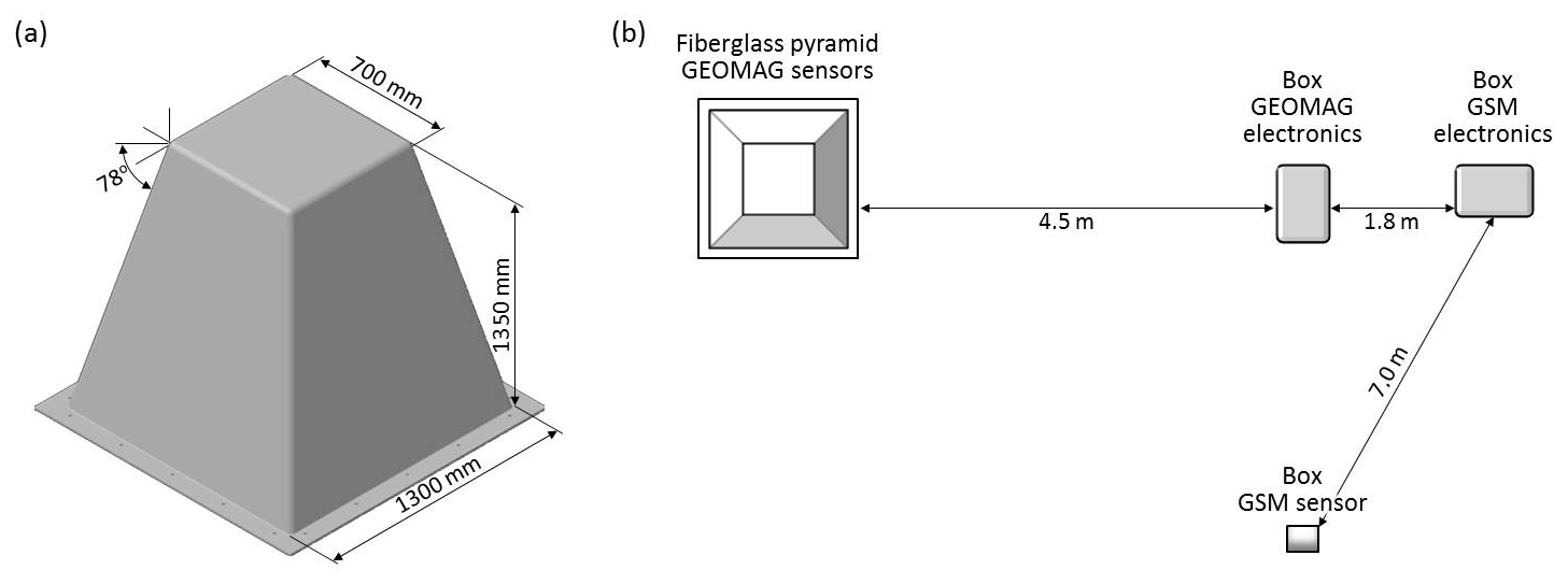
Figure 4 Fibreglass pyramid dimensions constructed for the Macapá magnetometer station (a) and schematic locations of the fibreglass pyramid with GEOMAG sensor, boxes with GEOMAG and GSM electronics, and the box with the GSM sensor (b).

3 Macapá dataset

Data from Macapá station (MAA) were recorded from 14 November 2019 until 25 July 2022 with an availability of 93 % for scalar data and 35 % for the vector data. The time distribution of the MAA dataset is shown in Fig. 5.

Figure 5 Temporal distribution of the scalar (GSM, green) and vector (GEOMAG, red) data available at the Macapá magnetometer station. The vertical dashed line indicates the starting time of the synchronisation problem.

Since GEOMAG stopped transmitting data automatically via its serial RS-232 port on 5 December 2019, the data needed to be transferred by exchanging CF cards once a week. From this time on, the recording by the vector magnetometer had several interruptions due to technical problems such as damage to the GPS. Because of high temperatures in Macapá and insufficient shading of the electronics box, the GEOMAG-02 electronics inside it reached more than 50 °C, exceeding its maximum operating temperature of 40 °C as recommended by the manufacturer.

The GPS of the GEOMAG stopped working on 23 January 2021. This caused a time shift problem in the vector magnetic data (see example in Fig. 6). Since the GSM scalar data have correct time stamping, we could apply a correction to synchronise both signals. To do so, we apply the following sequence.

• i.

  Obtain a first approximation of the delay by finding for each day the time difference in the maxima in calculated F of the fluxgate and the measured F data of the Overhauser.

• ii.

  Systematically shift the time correction for the vector data, starting from the approximate delay found in (i) and calculating the correlation between the shifted calculated F data and the measured F data.

• iii.

  For each day, select the time stamp correction with the highest correlation.

• iv.

  For the whole period, perform a least-squares fitting using a spline on the selected time stamp corrections from (iii).

• v.

  The performed fitting will yield a smoothed time error correction for the whole period.

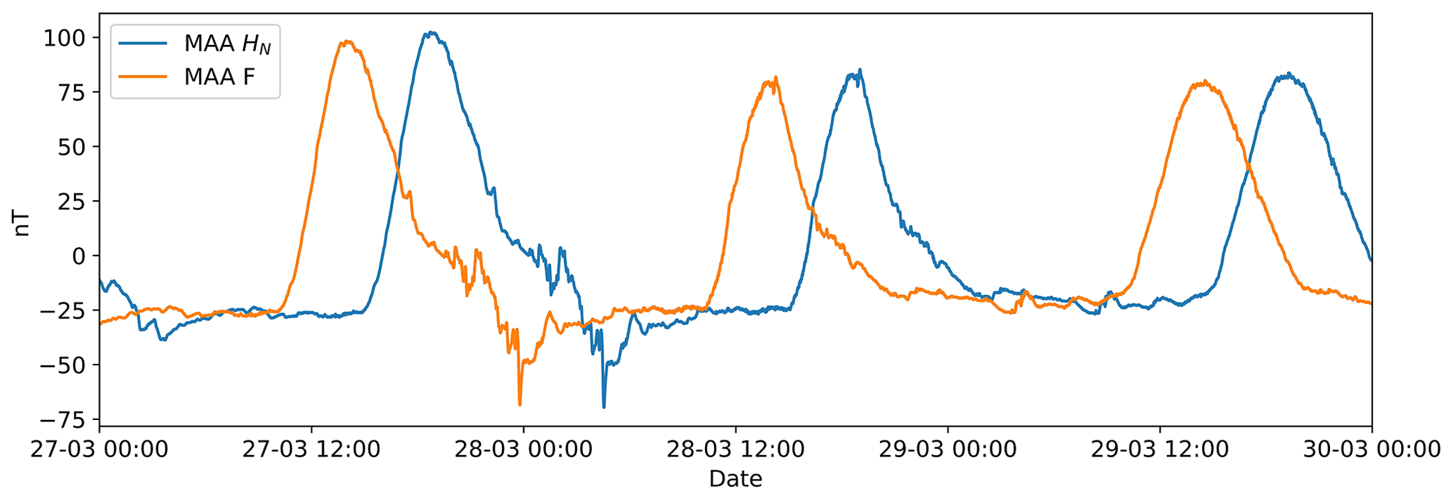
Figure 6 Example of a time shift caused by a GPS problem in Macapá station. The total field F was measured by the scalar magnetometer GSM and H_N by the vector magnetometer GEOMAG.

Figure 7 Example of artificial disturbance on 17 January (a) shown in H_N of MAA (blue line) compared to no disturbed signal in H_N of TTB (green line) and total field (F) at MAA (orange line). The first time derivative (b) of the H_N of MAA and TTB and F in MAA.

After synchronisation, we removed spikes and artificial disturbances from the data. Spike amplitudes exceeding 1 nT were removed. Spikes were detected by visually checking the first time derivative of each component. Artificial disturbance was visually identified in the geomagnetic data and its first time derivative and manually removed (see example in Fig. 7).

After the removal of spikes, MAA data were visually compared to TTB, showing a good agreement of H_N and H_E and a certain degree of anti-correlation in Z (Fig. 8), as is expected from the station location and the geometry of the equatorial ionospheric current system. Both TTB and MAA are under the influence of the EEJ (see Fig. 1), presenting a very similar effect of H-component amplification (Fig. 8). Kourou (KOU) is the closest magnetic observatory from TTB, but it is still far from the magnetic equator and is therefore free from the effects of the EEJ. It is possible to isolate the localised EEJ effect from large-scale magnetospheric and large-scale solar quiet (Sq) signal by subtracting the data of KOU from the MAA magnetometer station (see, e.g. Morschhauser et al., 2017; Soares et al., 2018). We calculated the differences between the horizontal components of MAA and KOU and TTB and KOU (Fig. 9). The differences indicate the intensity of the EEJ signal, which here is around 60 nT (peak to peak). Note that the difference for MAA is slightly greater than for TTB, indicating that the EEJ effect is slightly larger in MAA than in TTB.

Figure 8 Comparison between the data of TTB (blue) and MAA (red) from 9–14 January 2020 for H_N (a), H_E (b), Z (c), and F (d).

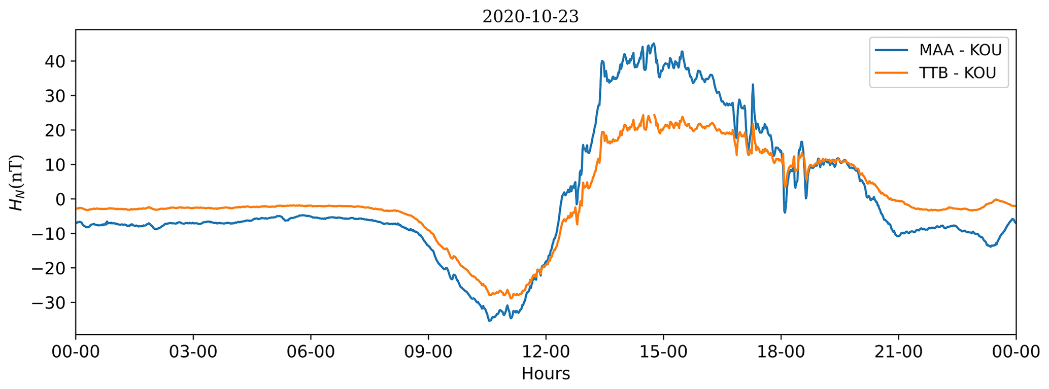
Figure 9 Differences between the horizontal components of Macapá (MAA) and Kourou (KOU) (blue line) and Tatuoca (TTB) and Kourou (brown line).

4 Temperature correction

The total magnetic field is measured directly by the scalar magnetometer (here denoted as F_s, measured by GSM-90; see Appendix A), which is assumed to be temperature invariant (Jankowski and Sucksdorff, 1996). It can also be calculated using the three components recorded by the vector magnetometer (here denoted as F_v, measured by GEOMAG). The temperature is measured in the pyramid (GEOMAG sensor, T_s) and in the box (GEOMAG electronics, T_e). Hourly mean values T_a of ambient temperature are measured by the Instituto Nacional de Meteorologia less than 2 km from the magnetometer station. All the variable and constant parameters used in this paper are listed in Appendix A. The electronic temperature is higher and more variable with time compared to sensor temperature (Fig. 10). They also show a time shift between the temperature peaks, which occur earlier in the electronics temperature. This happens because the electronics produce more heat and are less insulated from ambient temperature changes. Figure 10 shows the two temperature signals varying with time.

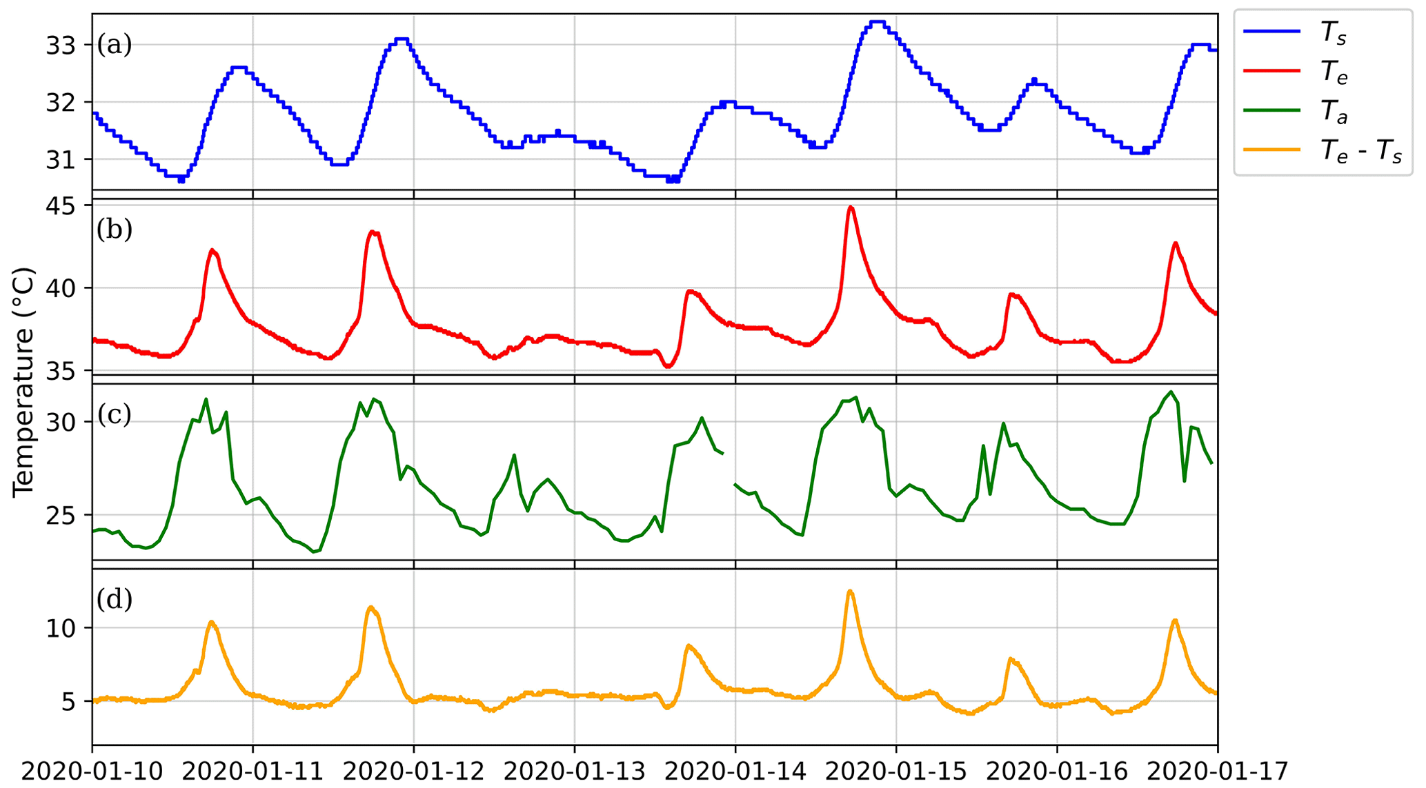
Figure 10 Temperature variation of the GEOMAG sensor (a), GEOMAG electronics (b), and ambient temperature (c) and the difference between temperature of the GEOMAG electronics and the sensor (d). The temperature variations are shown for 10–16 January 2020.

The calculated total field (F_v, Appendix A) using the three vector components is obtained by

$$\begin{array}{}\text{(1)}& F_{\mathrm{v}}\left(t\right)={\left[{\left(H_{{\mathrm{N}}_{\mathrm{0}}}+H_{\mathrm{N}}\left(t\right)\right)}^{\mathrm{2}}+H_{\mathrm{E}}(t{)}^{\mathrm{2}}+{\left(Z_{\mathrm{0}}+Z\left(t\right)\right)}^{\mathrm{2}}\right]}^{\mathrm{0.5}},\end{array}$$

where t is time and $H_{{\mathrm{N}}_{\mathrm{0}}}$ and Z₀ are the sensor offsets (also called baselines) of the north sensor and the vertical sensor, respectively. Note that the east sensor has a negligible small offset, which we set to 0 here. The baselines $H_{{\mathrm{N}}_{\mathrm{0}}}$ was obtained by subtracting a typical value of H_N during nighttime and during quiet geomagnetic conditions from the simultaneous H value determined by the IGRF-13 model for the location of Macapá. The baseline Z₀ was determined in an analogue fashion. The difference between the calculated (F_v) and the observed scalar (F_s) total fields is denoted as follows:

$$\begin{array}{}\text{(2)}& \mathrm{\Delta }{F}_{\mathrm{0}}\left(t\right)=F_{\mathrm{v}}\left(t\right)-F_{\mathrm{s}}\left(t\right).\end{array}$$

Figure 11 Macapá magnetometer station differences (ΔF₀ to ΔF₃) between the calculated total fields ($F_{{\mathrm{v}}_{\mathrm{0}}}$ to $F_{{\mathrm{v}}_{\mathrm{3}}}$) and the scalar total field (F_s), from (a)–(d), respectively. In (b) and (c) the left y axis corresponds to ΔF_v, while the right y axis corresponds to the sensor temperature in b and to the difference in the electronics and sensor temperatures in c. All the ΔF_v values are plotted together in (e). The period shown in this example is from 10–17 January 2020.

This difference should be zero if both instruments perform their measurements correctly. But for Macapá station setup it varies with a daily periodicity, as exemplified in Fig. 11a. In order to obtain a possible scaling factor a₁ and offset b₁ between both signals, we minimise using least squares:

$$\begin{array}{}\text{(3)}& \min \left|\mathrm{\Delta }{F}_{\mathrm{0}}\right(t\left)\right|={\left[\sum _{t=\mathrm{1}}^M{\left(\left(a_{\mathrm{1}}{F}_{\mathrm{v}}\left(t\right)+b_{\mathrm{2}}\right)-F_{\mathrm{s}}\left(t\right)\right)}^{\mathrm{2}}\right]}^{\mathrm{0.5}}\sim \mathrm{0},\end{array}$$

and we determine the coefficients by linear regression. We apply this correction to 5 d moving window for all MAA data (The MathWorks Inc., 2018). We found that a₁ values are 0.964±0.015 and that b₁ is negligible ($\sim {\mathrm{10}}^{-\mathrm{4}}$ nT).

$$\begin{array}{}\text{(4)}& \mathrm{\Delta }{F}_{\mathrm{1}}\left(t\right)=F_{{\mathrm{v}}_{\mathrm{1}}}\left(t\right)-F_{\mathrm{s}}\left(t\right)\end{array}$$

The above equation still contains a periodic signal that is correlated to the sensor temperature (T_s), as shown in Figs. 11b and 12.

There is no significant temperature variation between 12 and 13 January 2020 (Fig. 10). However, in the same days the ΔF₀ varies with time (Fig. 11a), indicating that there is a diurnal geomagnetic variation besides temperature variation. In order to remove the T_e signal, we minimised ΔF₁ and obtain the a₂ coefficient via linear regression (Appendix A):

$$\begin{array}{}\text{(5)}& \begin{array}{rl}\min \left|\mathrm{\Delta }{F}_{\mathrm{1}}\right(t\left)\right|& =\left[\sum _{t=\mathrm{1}}^M\left(\left(F_{{\mathrm{v}}_{\mathrm{1}}}\left(t\right)-a_{\mathrm{2}}{T}_{\mathrm{s}}\left(t\right)+b_{\mathrm{2}}\right)\right.\right.\\ & {\left.{\left.-F_{\mathrm{s}}\left(t\right)\right)}^{\mathrm{2}}\right]}^{\mathrm{0.5}}\sim \mathrm{0},\end{array}\end{array}$$

where typical values of a₂ are $-\mathrm{0.3}\pm \mathrm{0.15}$ nT °C⁻¹ and b₂ is negligible ($\sim {\mathrm{10}}^{-\mathrm{9}}$ nT) in all datasets. We expected that $F_{{\mathrm{v}}_{\mathrm{2}}}\left(t\right)=F_{\mathrm{s}}\left(t\right)$, where $F_{{\mathrm{v}}_{\mathrm{2}}}\left(t\right)=F_{{\mathrm{v}}_{\mathrm{1}}}\left(t\right)-a_{\mathrm{2}}{T}_{\mathrm{s}}\left(t\right)$. However,

$$\begin{array}{}\text{(6)}& \mathrm{\Delta }{F}_{\mathrm{2}}\left(t\right)=F_{{\mathrm{v}}_{\mathrm{2}}}\left(t\right)-F_{\mathrm{s}}\left(t\right),\end{array}$$

is still a periodic signal strongly correlated to the difference between the electronic temperature (T_e) and sensor temperature (T_s), as exemplified in Fig. 11. In order to remove the T_e−T_s signal, we minimised ΔF₂ and obtain the a₃ coefficient via linear regression:

$$\begin{array}{}\text{(7)}& \begin{array}{rl}\min \left|\mathrm{\Delta }{F}_{\mathrm{2}}\right(t\left)\right|& =\left[\sum _{t=\mathrm{1}}^M\left(F_{{\mathrm{v}}_{\mathrm{2}}}\left(t\right)-a_{\mathrm{3}}\left(T_{\mathrm{e}}\left(t\right)-T_{\mathrm{s}}\left(t\right)+b_{\mathrm{3}}\right)\right.\right.\\ & {\left.{\left.-F_{\mathrm{s}}\left(t\right)\right)}^{\mathrm{2}}\right]}^{\mathrm{0.5}}\sim \mathrm{0},\end{array}\end{array}$$

where a₃ typical values are $-\mathrm{0.04}\pm \mathrm{0.025}$ and b₃ is also negligible ($\sim {\mathrm{10}}^{-\mathrm{12}}$ nT) for all datasets. Therefore,

$$\begin{array}{}\text{(8)}& \mathrm{\Delta }{F}_{\mathrm{3}}\left(t\right)=F_{{\mathrm{v}}_{\mathrm{3}}}\left(t\right)-F_{\mathrm{s}}\left(t\right)\sim \mathrm{0},\end{array}$$

where $F_{{\mathrm{v}}_{\mathrm{3}}}\left(t\right)=F_{{\mathrm{v}}_{\mathrm{2}}}\left(t\right)-a_{\mathrm{3}}\left(T_{\mathrm{e}}\right(t)-T_{\mathrm{s}}(t\left)\right)$. Finally, the complete expression for the corrected calculated total field value F_v is as follows:

$$\begin{array}{}\text{(9)}& {\stackrel{\mathrm{̃}}{F}}_{\mathrm{v}}\left(t\right)=a_{\mathrm{1}}{F}_{\mathrm{v}}\left(t\right)-a_{\mathrm{2}}{T}_{\mathrm{s}}\left(t\right)-a_{\mathrm{3}}\left(T_{\mathrm{e}}\left(t\right)-T_{\mathrm{s}}\left(t\right)\right),\end{array}$$

which can be rewritten as

$$\begin{array}{}\text{(10)}& {\stackrel{\mathrm{̃}}{F}}_{\mathrm{v}}\left(t\right)=a_{\mathrm{1}}{F}_{\mathrm{v}}\left(t\right)-\left(a_{\mathrm{2}}-a_{\mathrm{3}}\right)T_{\mathrm{s}}\left(t\right)-a_{\mathrm{3}}{T}_{\mathrm{e}}\left(t\right),\end{array}$$

which is the more classical form of describing the temperature dependency of a magnetometer as it assigns a coefficient to the sensor temperature and the electronics temperature. In addition, INTERMAGNET suggests to monitor both sensor and electronics temperatures and to use these values for correction purposes (St-Louis et al., 2020, p. 10 and 11).

The critical point is that the sensor and electronics temperatures both depend on the ambient temperature. Therefore, they are not independent, and at the same time they do not have the same shape (Fig. 10a and b). This is because they have different insulation that creates a delay in the temperature maximum. After the correction of T_s, we remove part of the dependency on T_e, but there is still a signal corresponding to the difference between the temperatures (Fig. 10d) that needs to be removed. Now we can compare the observed temperature coefficients (typical values are $a_{\mathrm{2}}=-\mathrm{0.3}\pm \mathrm{0.15}$ nT °C⁻¹ and $a_{\mathrm{3}}=-\mathrm{0.04}\pm \mathrm{0.025}$) with the temperature coefficient given by the manufacturer. If the sensor and electronics are operating at the same temperature, the observed temperature coefficient will be around $a_{\mathrm{2}}=-\mathrm{0.3}\pm \mathrm{0.15}$ nT °C⁻¹. This is close to the instrument specification of <0.2 nT °C⁻¹ given by the manufacturer for the GEOMAG-02 fluxgate.

It should also be noted that in the Macapá setup T_s and T_e remain different due to other factors like uneven sun exposure on the pyramid and on the box. This occurs because of the different shading by trees (albedo). Another factor is self-heating of the electronics, which is assumed to be a constant temperature change. We analyse the correlation between the different temperature signals with F_s to confirm the most appropriate correction sequence, as shown in Fig. 12a. Figure 12b quantifies how the misfit between F_s and the different F_v decreases with each correction. It would be preferable to determine a temperature coefficient for each of the three sensors of the GEOMAG-02. However, due to the location at the geomagnetic equator and because the instrument is oriented along magnetic north, the temporal change measured by the north sensor H_N corresponds very closely to the temporal change measured by the scalar magnetometer. At the same time, both H_E and Z₀+Z measure very small magnetic fields and hardly contribute to F_v. Therefore, the temperature coefficients determined here can be attributed to the H_N sensor, while the temperature coefficients of the H_E and Z sensor remain undetermined.

Figure 12 Correlation of ΔF₁ (left panel), ΔF₂ (middle panel), and ΔF₃ (right panel) with sensor temperature T_s, electronics temperature T_e, and T_e−T_s in blue in (a). RMSE (root-mean-square error) for each ΔF is given in (b).

5 Conclusions

In this paper, we presented the new magnetometer station in Macapá (northern Brazil) built as a result of collaboration between the National Observatory (ON – Brazil), the Federal University of Pará (UFPA – Brazil), and the German Research Centre for Geosciences (GFZ – Germany). Macapá station is especially relevant because of the rapid temporal variation of the magnetic equator in the Brazilian longitudinal sector. The magnetic equator passed over Tatuoca observatory (TTB) in 2012 and continued to move northwards. Today it is located between Macapá station and Tatuoca observatory (Fig. 1). The IGRF model forecasts that the magnetic equator will continue to move northwards and pass by Macapá station in 2024. The presence of the magnetic equator causes another phenomena called the equatorial electrojet (EEJ), responsible for H-component amplification. Since Kourou magnetic observatory is out of the influence of the EEJ, it does not record the H-amplification, as it is observed in Tatuoca magnetic observatory (Fig. 2) and Macapá station.

At Macapá station we measured the total magnetic field (F) with a scalar magnetometer (GSM) and the three components (H_N, H_E and Z) with a vector magnetometer (GEOMAG). The sensor and electronics for each magnetometer were installed in different huts (Fig. 3). The GEOMAG sensor was inside a fibreglass pyramid about 5 m from the electronics box (Fig. 4). We recorded data from Macapá station from November 2019 until September 2021 (Fig. 5). There were some problems in the data acquisition, such as a GPS failure that caused a time shift between the data of GEOMAG and GSM (Fig. 6). The time shift and other problems in the data, such as noise and spikes (example in Fig. 7), were corrected. Macapá data were then compared with TTB, which is the closest observatory. The data of TTB and Macapá showed good agreement (Fig. 8), which helps to assure the quality of the recorded data.

In order to measure the amplitude of the equatorial electrojet (EEJ), we subtract the data from Macapá station and TTB, both under the influence of the EEJ, from Kourou observatory (Fig. 9). The EEJ signal was recorded at Macapá with a similar amplitude to that at TTB.

Because of the particular setup configuration of Macapá (Fig. 3), we got very different values for the temperature of the (GEOMAG) sensor and electronics (Fig. 10), and presumably these temperature variations influence the Macapá data. We implement a methodology considering two types of correction in the data: diurnal variation (between GEOMAG and GSM – included in ΔF₀) and temperature variation (included in ΔF₁ and ΔF₂), as shown in Fig. 11. The results demonstrate that there is a high correlation between the difference in GEOMAG and GSM with the temperature of the sensor and electronics and the difference between them (Fig. 12). Therefore, it is important to consider that variations in temperature may affect the data of magnetic stations, and it may be important to apply a correction.

Appendix A: Notation used in this paper for each variable and constant parameters

Notation	Description
Fs(t)	Observed scalar total field recorded by the
	GSM
HN(t)	Horizontal north magnetic field in the sensor
	coordinate system
HE(t)	Horizontal east magnetic field in the sensor
	coordinate system
Z(t)	Vertical magnetic field
Te(t)	Electronic temperature measured inside the
	box (GEOMAG)
Ts(t)	Sensor temperature measured inside the
	pyramid (GEOMAG)
Ta(t)	Ambient temperature of Macapá station
Fv(t)	Calculated total field using the three
	vector components of GEOMAG
$F_{{\mathrm{v}}_{\mathrm{1}}}\left(t\right)$	Fv(t) corrected by linear regression using
	Fs(t)
$F_{{\mathrm{v}}_{\mathrm{2}}}\left(t\right)$	$F_{{\mathrm{v}}_{\mathrm{1}}}\left(t\right)$ corrected by linear regression using
	Ts(t)
$F_{{\mathrm{v}}_{\mathrm{3}}}\left(t\right)$	$F_{{\mathrm{v}}_{\mathrm{2}}}\left(t\right)$ corrected by linear regression using
	(Te(t)−Ts(t))
${\stackrel{\mathrm{̃}}{F}}_{\mathrm{v}}\left(t\right)$	Corrected calculated total field value (final)
ΔF0(t)	Difference between Fv(t) and Fs(t)
ΔF1–3(t)	Differences between $F_{{\mathrm{v}}_{\mathrm{1}\text{–}\mathrm{3}}}\left(t\right)$ and Fs(t)
(a,b)1–3	Linear regression coefficients
$H_{{\mathrm{N}}_{\mathrm{0}}}$	Baseline value of the horizontal component
	calculated by the IGRF model
Z0	Baseline value of the vertical component
	calculated by the IGRF model