Modular approach to near-time data management for multi-city atmospheric environmental observation campaigns

Urban observation networks are becoming denser, more diverse, and more mobile, while being required to provide results in near time. The Synergy Grant “urbisphere” funded by the European Research Council (ERC) has multiple simultaneous field campaigns in cities of different sizes, collecting data to improve weather and climate models and services, including assessing the impact of cities on the atmosphere (e.g., heat, moisture, pollutant, and aerosol emissions) and people's exposure to extremes (e.g., heat waves, heavy precipitation, air pollution episodes). Here, a solution to this challenge for facilitating diverse data streams from multiple sources, scales (e.g., indoors, regional-scale atmospheric boundary layer), and cities is presented.

For model development and evaluation in heterogeneous urban environments, we need meshed networks of in situ observations with ground-based and airborne (remote) sensing platforms. In this contribution we describe challenges, approaches, and solutions for data management, data infrastructure, and data governance to handle the variety of data streams from primarily novel modular observation networks deployed in multiple cities, in combination with existing data collected by partners, ranging in scale from indoor sensor deployments to regional-scale boundary layer observations.

A metadata system documents (1) sensors and instruments, (2) the location and configuration of deployed components, and (3) maintenance and events. This metadata system provides the backbone for converting instrument records to calibrated, location-aware, convention-aligned, and quality-assured data products, according to FAIR (findable, accessible, interoperable, and reusable) principles. The data management infrastructure provides services (via, e.g., Application Programming Interface – APIs, apps, integrated computing interfaces – ICEs) for data inspection and subsequent calculations by campaign participants. Some near-real-time distributions are made to international networks (e.g., AERONET, PhenoCam) or local agencies (e.g., GovDATA) with appropriate attribution. The data documentation conventions, used to ensure structured datasets, in this case are used to improve the delivery of integrated urban services, such as to research and operational agencies, across many cities.

1 Introduction

Field observation campaigns are an essential source of information in urban environments, as long-term global climate and weather observation networks often explicitly exclude cities (Grimmond et al., 2020). Urban field campaigns differ in length, providing different benefits. For example, short (approximately 1 year) campaigns offer a cost-effective way to explore seasonal variability in multiple urban areas by relocating instruments, whereas long-term observatories allow changes from both climate and the city itself (e.g., physical, behavioral) to be better understood. Data of both types are needed to support model development for numerical weather and climate predictions as well as the delivery of integrated urban services (Baklanov et al., 2018) to support current operations, plan management (Chrysoulakis et al., 2023), and adaptation of cities into the future. Such observation campaigns require robust, structured data management. Unlike operational regulatory networks (e.g., air quality), campaigns have limited duration and often employ novel measurement systems before open-source or commercial data management solutions exist.

Urban environments pose challenges because of multiple scales of interest (indoors to city-wide), intra-city and intercity diversity at most scales (e.g., room uses, building types, neighborhoods), and people's activities (e.g., needing to continue undisturbed but impacts observed), and all of these are compounded by city size (Landsberg, 1970; Oke, 2005; Grimmond, 2005; Muller et al., 2013b; WMO, 2019; Yang and Bou-Zeid, 2019; Masson et al., 2020; Grimmond et al., 2020). Existing long-term sensors, enhanced for campaign objectives and applications (e.g., human health, energy infrastructure), allow urban surface–atmosphere dynamics to be captured. However, the multitude of city layouts, topographic settings, and regional climates means there is not one solution to combining field observations, remote sensing, and modeling in urban areas. Rather there is need to address this at multiple scales simultaneously, in multiple cities with duplication of combinations to ensure the general pattern is correctly identified (Barlow et al., 2017; Pardyjak and Stoll, 2017; WMO, 2021) in comparisons. Hence, concurrent sensor deployments, mounted on static and mobile platforms, located indoors and outdoors, measuring microscale to mesoscale processes over different length of periods, will need to occur.

Research campaigns by definition deviate from operational deployments (e.g., the WMO's National Meteorological and Hydrological Services). Urban campaigns have a long tradition of multiple groups combining resources to focus on a city or a specific aspect of the urban environment (e.g., Changnon et al., 1971; Rotach et al., 2005; Allwine et al., 2004; Mestayer et al., 2005; Wood et al., 2013; Bohnenstengel et al., 2015; Scherer et al., 2019; Karl et al., 2020; Caluwaerts et al., 2021; Fenner et al., 2024b), making a homogeneous single-sensor model network, operated by multiple collaborating partners using identical operating protocols (e.g., same objectives, calibration procedures), unlikely (Scherer et al., 2019; Caluwaerts et al., 2021; Marquès et al., 2022). Although sensors designed for the same observation type may be similar, they are rarely fully interchangeable (de Vos et al., 2020). However, intentionally heterogeneous sensor model networks (e.g., low-cost and high-grade instruments) may complement each other (Jha et al., 2015; Gubler et al., 2021).

Data collection by a single project in one city should produce data comparable to those collected in other cities, or a later campaign in the same city, to support comparative and longitudinal studies. The large datasets need to be easily ingestible into model evaluation studies today and in the future, requiring structured data and attributed metadata following conventions and standards.

Short-term urban field observation campaigns are highly dynamic (Yang and Bou-Zeid, 2019), capturing processes of interest and responding to near-real-time results, allowing plans to evolve. The dynamics make data assessments time-sensitive and performing network operational status diagnostics a critical task, as intermediate results become indispensable for informing models, making decisions on resource-intensive field deployments (e.g., radiosoundings, tracer releases), and making dynamic adjustments to network design (Changnon et al., 1971; Rotach et al., 2005). Data management for rapid discovery needs to be both technically and organizationally structured, posing additional challenges (Wilkinson et al., 2016; Middel et al., 2022). In a research community, sharing near-real-time data internally and publicly is increasingly expected, as data, software code, and products (results) are co-produced. Thus, output becomes “living data” given continuous sharing, even before all required metadata are available (Oke, 2005; Stewart, 2011; Muller et al., 2013a; WMO, 2023) including attribution, documentation in peer-reviewed papers, or full scientific scrutiny. However, rapid availability does not remove scientific obligations (e.g., peer-reviewed publications with careful scientific assessment, attribution to researchers, institutions, funding agencies).

Here, we present an approach developed within the European Research Council (ERC) Synergy Grant “urbisphere”. The urbisphere grant addresses dynamic feedback between weather, climate, and cities through synergistic activities among four disciplines (spatial planning, airborne and spaceborne observations, modeling, and ground-based observations). The project involves quantifying aspects of the influence of urban emissions on the atmospheric boundary layer above and downwind of cities and human exposure in urban environments (e.g., streets, indoors) that vary across a city and with time as both form and function change.

Central to urbisphere are both concurrent and consecutive campaigns in multiple cities undertaken in different countries using a modular observation system. Observations are needed to support empirical assessments and studies, model development, and model evaluation. Activities are structured into four modules (A to D; Fig. 1). Module A gathers data on urban form (e.g., morphology, materials) and function (e.g., people’s mobility patterns, vegetation phenology), which vary in space and over time. Data from surveys, official sources, imagers, and spaceborne sensors are used to geographically and temporally assess form and function and to derive inputs to models. Module B quantifies how urban form and function affect the urban atmosphere over and downwind of cities through emissions of heat, pollutants, and aerosols and how cities modify the dynamic and thermodynamic state of the overlying atmospheric boundary layer. In Module C, we quantify the differential exposure of people in and between cities (e.g., to heat, flooding). The different objectives in Modules A to C require targeted and specific observational strategies, but all require consistent data management, documentation, and quality control processes (Module D).

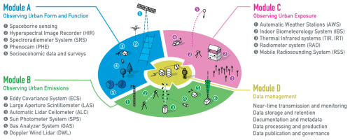
Figure 1 Conceptual diagram of the modular observation system operated in the urbisphere project. Modules A to C collect observational data in different cities, and Module D integrates them in the unified data management approach.

Here we present the integrating data management and infrastructure system (Module D) developed to support the observational sensors and systems in Modules A to C (Fig. 1). We exclude spaceborne observations, data from long-term partner data networks (e.g., meteorological agencies and services), and surveys and administrative data as there are existing data management platforms and systems available. Instead we focus on atmospheric and environmental sensing systems in Modules A to C that are deployed during campaigns. The observational sensors and systems deployed in Modules A to C are diverse (Fig. 1), quantifying many variables, and are operated in diverse settings (e.g., street-light posts, building rooftops, indoors) as well as on mobile platforms (e.g., vehicles, balloons, drones). Hence, there are fixed deployments and mobile measurements, sensors with multiple uses, needs for near-real-time data (e.g., during intensive observation periods – IOPs), and changing configurations with deployments of varying duration (e.g., hours, days, months, years). This is managed by multiple people with different responsibilities, roles, and backgrounds.

The system currently ingests on the order of 10⁹ data points per day from about 100 different stations and approximately 1000 sensors in five different cities. Using automated processes, data are delivered in near time (minutes to hours) to central data infrastructure through mobile phone and Internet of Things (IoT) connectivity. We showcase the technical and organizational solutions to creating a modular data management system, considering documentation, acquisition, products, governance, standardization, reuse, and sharing.

2 Data documentation

As data documentation during observation campaigns occurs at pre-deployment, during deployment, and at post-deployment, it is critical to have a structure early for capturing all details (e.g., Table 1), especially in busy, time-limited periods. As part of sensor installation preparation, data to describe a site and sensor system details need to be captured, as they are essential metadata for processing the data stream. Standard conventions facilitate data (re)use, enhancing data value for both the general community and the project (Muller et al., 2013a; WMO, 2021). Critical to this is the accessibility of data to team members during a campaign and subsequently as data are processed (Fig. 2).

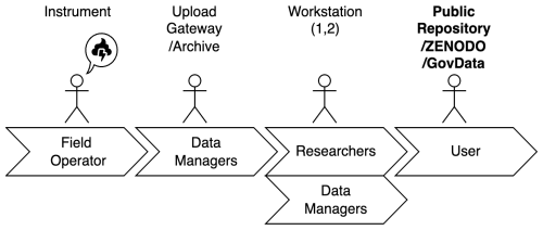
Figure 2 Operational connections are entwined between the physical and logical networks and the organizations.

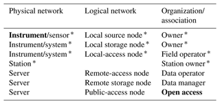
Table 1 The provenance of each field observation can be mapped within an infrastructural, a logical, and an organizational network. The connections and associations between the origin and the data product (both in bold) are not limited to the field situation (indicated by an asterisk).

2.1 Metadata

As field observations involve multiple networks (Table 1), metadata are essential to organizing the data collection (e.g., files, directories) and as the audit trail of modifications. Because of the latter, the physical, logical, and organizational contexts of the field observations are defined early in the data management process (Table 1) and amended with updates from planning to collection to publication. Once data collection begins, the production chain needs to systematically encode attributes (e.g., location) into a series of searchable metadata databases (DBs; Fig. 3).

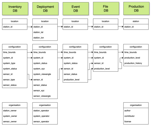
Figure 3 Conceptual overview of databases (DBs) that form the metadata and the primary attributes that connect the DBs.

The inventory DB has all instruments used in the campaigns with links to the maintenance and organization details (e.g., owners of different parts of a deployment; Fig. 3). The inventory DB holds the primary calibration, purchasing, maintenance, and software (firmware) history and availability of each instrument. The operational relational queries are supported by graphical user interfaces (GUIs) with shortcuts for specific summaries. Those help find, e.g., (1) if an identical instrument model exists in storage or in another deployment, (2) all instruments at a location, (3) all mobile phone SIM cards linked to a data plan, and (4) all calibration sheets and warranty documents for a given sensor to facilitate sending an instrument back to a manufacturer for service. The inventory GUI offers dialog in multiple languages, facilitating international cooperative use by all staff, and incorporates direct access to all instrument manuals.

The deployment DB (Fig. 3) has information about an instrument's configuration, including location and relation to other instruments during a deployment, as well as organization details. This is the primary record of instrument operational status at any time. The deployment DB GUI allows entries to be added or modified. Most instruments are in a hierarchical relation, such as being a “child” connected a “parent” (e.g., internet-attached data logger connected to an instrument). A two-level parent–child hierarchy has instruments on a local network node with a local storage node referred to as a “system” (Tables 1 and 2). For the deployment DB consistency, instruments with integrated data recording and autonomous network capabilities are both a system and a “sensor”.

The hierarchy of spatial information for a “station” (or “site”) starts with geographic coordinates of a point on a representative surface, which can be determined accurately in advance to ensure suitability for sampling by (airborne) remote sensing. The system and sensor are measured in relation to the site in a local Cartesian or polar coordinate system (Fig. A3). This helps explain details in a complex setting such as on a roof (Fig. A1), in a street canyon, or within a building (Fig. A2). The database relationships allow identical sensor replacement, without needing to modify any of this spatial information. Typically, a duplicate configuration is modified to capture the changes occurring for a period. Given numerous complementary data sources, including spaceborne and airborne sources (e.g, satellites, drone, aircraft sensors), city GIS, and models (e.g., source areas, numerical weather prediction model output), it is critical that metadata are precisely geolocated and time-stamped. In the deployment DB, the start time and end time identify the operational periods (Fig. 4).

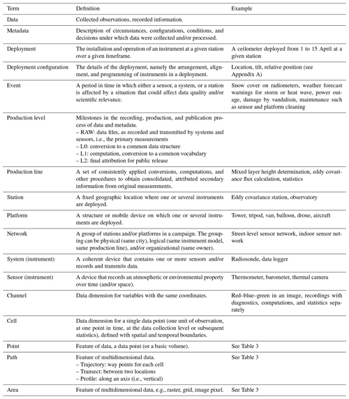
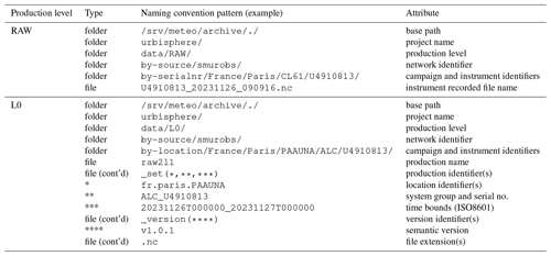
Table 2 Observational network data are organized using a limited set of dimensions, (typically) retrieved from the data themselves and their associated metadata. Ingested data (RAW) are completed across the multidimensional data stores at level 0 (L0). Although metadata are essential for data analysis, they are not repeated at all levels (L) to improve interoperability.

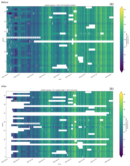
Figure 4 Example of data (air temperature) through time per station deployed (Freiburg, Germany): (a) pre- and (b) post-metadata application for masking invalid data. In this case, the instruments (autonomous automatic weather stations) report data if powered, so metadata are needed to define operational deployment periods.

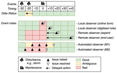
The event DB (Fig. 3) captures the field and laboratory notes, normally linked to events, such as on-site maintenance visits, relevant near-site changes, remotely identified anomalies, and instrument disturbances (e.g., dirt on sensors). All field visits, instrument malfunctions, disturbances, anomalous weather, unexpected patterns in observed data, and brief data stream outages need to be documented as “events” at the time and may require subsequent actions. Complete documentation should provide a traceable audit trail of all intended and unexpected conditions related to an observed variable and, to facilitate subsequent data interpretation, measurement and photos of the location, orientation, direction of view, and relative position to obstacles, attributed with a time stamp. This information is vital to identifying and explaining unexpected changes or anomalous data. The collected event notes, after evaluation, if needed, are converted into deployment DB entries. Most events are not recorded in the event DB in real time because of varied paths, sources requiring decisions about the data consequences, and appropriate use (Fig. 5). Data stream quality control (QC) includes automated assessment of typical meteorological variables (e.g., air temperature, humidity, wind speed, wind direction, pressure, precipitation intensity), following, e.g., VDI (VDI 2013, see Appendix B). Event detection can include spatial statistics, but this is not operationally implemented. Documentation based on the metadata uses persistent identifiers and versioning in order to accommodate the advancing insights on quality, events, and deployment status (e.g., Plein et al., 2024).

Figure 5 Conceptual timeline (days, D) before and after an event is raised and resolved, with different examples of who is involved and when, including two automated methods (M1, M2).

2.2 Conventions

Building on existing data conventions and standards can enhance data usage. In urbisphere, we use the climate and forecast (CF) metadata convention (cf-conventions-1.10, or CF hereafter; see Hassell et al., 2017) Application Programming Interface (API) for NetCDF, with extensions often used in the urban research community (Scherer et al., 2019). The use is consistent with prior campaigns, model applications, and third-party software tools and is common among the campaign’s instruments and project-specific production needs.

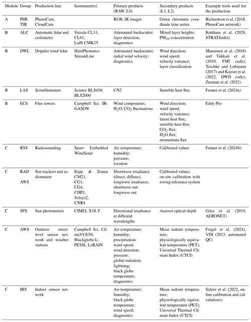
Most of the production chain in urbisphere is based on NetCDF database files. To maximize portability, only features commonly implemented in the various software libraries and platforms are used. A set of unique identifiers creates a relational chain between locations, instruments, events, variables, and variable units, and therefore the data recorded are publishable data products. To facilitate this, instruments and data are organized into functional groups (Fig. 1, Table 3; see also Appendix B).

Table 3 Instruments are classified into functional groups with sensors measuring at a point, along a path, or in a pixel area. Many instruments have dynamic source areas because of meteorological conditions or if the sensor is mounted on a mobile platform.

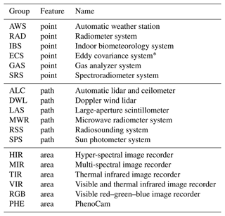
^* Can include a gas analyzer instrument.

Many instruments and data recorders encode sensor data records to proprietary formats, which based on user options may provide calibrated and aggregated data records with sensor diagnostics. To simplify later inquiries, a best practice for output file formats, metadata attributes, and file name patterns for each instrument model or instrument group (see, e.g., Appendix B) is adopted. Where possible, identifiers are included as headers in instrument data files, directory names, and/or file names. These practices allow programmatic extraction of key identifiers from file names as well as data and metadata databases with few exceptions. Particularly for observation systems that use APIs for the retrieval of data, consistent use of identifiers is an essential operational aspect (Feigel et al., 2024).

2.2.1 Vocabulary

CF forms a robust framework for data and metadata but does not formally include all variables needed in urban areas (Grimmond et al., 2010; Scherer et al., 2019, 2022; WMO, 2021; Lipson et al., 2022), so extensions are made by building on earlier projects that will need further review to be formally brought into the CF (Hassell et al., 2017). The shared vocabulary facilitates efficient queries and benefits for the machine operability of the data. The CF conventions define vocabulary for dimensions and units for many variables, as well as attributes to ensure data provenance (Hassell et al., 2017). Existing community software tools work with NetCDF and CF-related vocabulary definitions, including modules to perform programmatic conversion of units (e.g., the UDUNITS module; Hassell et al., 2017).

2.2.2 Outdoor deployment

Site selections in urban deployments depend on research questions, measured variables, and scales of interest (WMO, 2006; Oke, 2017). For example, the measurement of near-surface air temperature in an urban area may require different siting requirements than standard WMO regional-scale weather measurements (Stewart, 2011; WMO, 2023).

Most deployments are at fixed locations, but as surroundings change, regular review of deployment configurations is required, and time-specific amendments are needed to the metadata. Some instruments have accurate clocks and sensors to self-determine location and orientation, providing metadata as a separate time series in the data (e.g., pressure and GPS sensors on radiosounding systems; motor-drive position and inclinometer on lidar systems). Other deployments may require the sensor viewpoint and orientation as well as time offsets to be measured regularly or determined continuously relative to a (local) reference. Site documentation requires consistent use of coordinate reference systems, considering various aspects of urban landscapes and linkable to other sources (e.g., city GIS systems derived from detailed airborne lidars, numerical models) (Appendix A; Fig. A1). Local reference points are needed for all observations to be linked to other (e.g., geospatial) datasets. Some stations are located on surfaces (e.g., roofs) that may not coincide with the deployed platforms or instruments. However, using a representative surface coordinate set (Fig. A1b), instead of exact system location (Figs. A1a, A2), simplifies immediate reuse of coordinates between sources. Furthermore, some sensor views may not provide usable data for some research objectives, requiring detailed understanding of a site (e.g., glass or shaded areas for thermal imagery, orientation of a roof edge for momentum flux, three-dimensional scan patterns for Doppler wind lidar). All systems have GPS time or internet reference time services, and all data during urbisphere campaigns are recorded in Coordinated Universal Time (UTC), Greenwich Mean Time (GMT), or the GMT (UTC+00:00) locale without daylight savings for systems with time-zone-unaware recording of time stamps (Appendix A1).

2.2.3 Indoor deployment

Sensors deployed indoors have multiple purposes including assessing human exposure (Sulzer et al., 2022), building energy models (Liu et al., 2023), and influences of the indoor micro-climate extremes on human and animal stress (Walikewitz et al., 2015; Marquès et al., 2022; Sulzer et al., 2023), so they require many site details. A classification is implemented that includes characteristics and orientation of the building, room, walls, windows, contents of the room, space usage type, occupancy, and other factors affecting the indoor climate and human comfort of workers or residents (Appendix A; Fig. A2). Whereas basic meteorological observations are recommended to be free of obstacles and heterogeneous influences, indoor observations are, in summary, the opposite. Siting for all sensors needs to be representative of what people and the room are likely to experience while still allowing the room to be used in its intended way.

2.3 Operational management

Conversations about planning, issues, and resolutions are an essential part of a campaign's knowledge base. To make communication related to the deployments accessible for discovery by data users, from any location and at any time, each campaign maintains a repository for issue tracking, source code development, and wiki-type documentation (GitHub, GitHub Inc; San Francisco, CA, USA). Similar repositories help maintain overarching subjects, such as data management. Other repositories are maintained on enterprise cloud data storage (Dropbox, Dropbox International Unlimited Company; Dublin, Ireland) to store and share auxiliary data files, such as photos, protocols, and calibration records, organized by campaign, location, and time. Additionally, customized forms and shareable spreadsheets are accessible using online services (Google Forms and Google Sheets, Google Ireland Limited; Dublin, Ireland) to gather provisional metadata.

The core database systems, including the inventory DB and deployment DB (Fig. 3), are designed using open-source web, database, and user-interface tools (the so-called LEMP stack; Linux, Nginx, MariaDB, PHP) and application frameworks (Appendix C3).

3 Data acquisition and products

A “data source” may be a sensor, a network node, or an organizational unit (Table 1), with different contexts that need to be retained and clearly identifiable. Typically, chains of systems and responsibilities are involved, with multiple actors, nodes, and locations (Tables 1, 3; Fig. 5). The origin of data may be expressed in terms of the physical network of infrastructure at distributed locations; the logical network involved in data telemetry, storage, and processing; and the network of organizations and actors who have various roles. The source needs to be defined and preserved in order to ensure data governance agreements, accessibility, and responsibilities and also to effectively respond to issues that occur. For example, if an instrument at a particular location is not responding, the data and metadata must allow the relevant infrastructure, the responsible people, and the production line processes to be looked up efficiently for that particular source (Fig. 2). Key features of the physical and logical networks (this section) are presented in terms of organizational aspects (Sect. 4).

3.1 Data infrastructure

The data infrastructure combines the interest of data safekeeping with data accessibility (Fig. 6). Keeping data secure is a primary project deliverable and involves basic protection against unknown malicious actors and protection against accidental data loss. Within the data architecture, a central operational archive is maintained on a suitably large storage volume (larger than 50 TB logical volumes on redundant storage units). A replica of the data is maintained on an identical storage unit in a different building (geo-redundant backup), with additional daily backups on enterprise storage services (on and off campus). The data infrastructure uses virtualized computing hardware. Virtualization makes it possible to isolate critical functions without the need to expand physical hardware and allows the data infrastructure to scale dynamically as needed. The critical functions include a remote-access node for all uploads from local field stations (“gateway”), a remote-access node for metadata databases and related web interfaces (“console”), and a remote storage node for archival of data and public-access nodes (“workstations”) for monitoring, computations, and user access to data (Fig. 6).

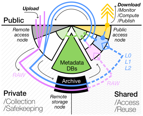
Figure 6 Access to data is needed from both public and private domains using private data infrastructure. Archived data and metadata are read-only accessible (dashed lines, light colors) for shared production (L0, L1, L2), which is redirected to the archive and interfaces for public access and other uses. DB: database

3.2 Access

The original data and metadata are kept on different physical servers. However, users with access to a workstation are provided with immediate access to a read-only view of the original data, as well as a read-only replica of the metadata DBs (Sect. 2.1). Access to data and metadata is read-only by default, primarily to minimize the risk of accidental data loss. This in turn removes the need for strict user access guidelines on the public-access node workstations, allowing more liberal use of the workstation resources. Workstations are used as public-access nodes, with a wide selection of services available at the user level, including APIs, integrated computing interfaces (ICEs), and other interactive websites (apps) for users and the public (see also Appendix C).

However, adding new files to the archive, or modifying files on the archive, is more involved and requires new or renewed upload. The uploaded data are managed by data managers using separate accounts for the upload and data management. Users and groups are managed at a file system level and the credentials are maintained in encrypted key chains for each campaign. The need for administrator privileges is avoided, where possible, and the access for accounts used in automation (e.g., File Transfer Protocol (FTP) credentials are transmitted as text) is restricted in scope. Write access to the remote storage node is restricted by default and limited in scope. Typically, data are uploaded automatically by an instrument, or manually by a user, onto intermediate storage locations on the remote storage node (“upload server”; see Fig. 6). Typically, uploads are synchronized immediately to dedicated locations on the archive. The synchronization uses individual configurations for each of the upload locations, which can be activated or deactivated if needed. Data management accounts are restricted in access scope to the relevant locations on the archive, set by file system permissions of the intermediate storage source and the destination location on the remote storage node. The design allows multiple campaigns to be operated at the same time without cross-interference and facilitates the transition in instrument deployment from one campaign to the next either by replacement of the user credentials for data upload on the local network node in the field or by reconfiguring the redirection destinations on the remote-access node. Such a transition between campaigns is helpful, as it allows the write access to original data locations to be revoked by a data manager after completion of one campaign, without the need to modify the individual file attributes of a complex subset of millions of files in file locations shared with subsequent campaigns.

3.3 Sources

Instrument groups are based on characteristic instrument features (Table 3). The three-character identifier is sufficient to prevent ambiguity.

Data are stored in the instrument-provided formats, which may be custom text records (encoded information in a proprietary format, e.g., TOA5, or a defined schema, e.g., XML), where new records are appended as lines to a file with a header that contains metadata and a column description. However, we have a preference for standardized delimited text files (e.g., comma-separated values) to simplify archival. Binary format files are used only where no text-based alternative exists. Binary formats are introduced where encoding is necessary to save storage space and bandwidth, including image formats for grid data and NetCDF format for trajectory data (Table 3). The data files contain collections of up to daily periods, except for the few cases with single time-stamp observations stored in separate files.

3.4 Transmission

Network connections for temporarily deployed instruments need to be flexible and modular. For a research network, temporary and long-term network outages must be accounted for in the design, requiring sufficient local data storage on or near the instrument, as well as methods to resume data transmission after an outage. The data recorded since the start of the network outage need to be transferred, ideally automatically. This requires methods that identify what is missing on the remote storage location and skip redundant uploading to save bandwidth. Although there are no substantial differences between text and binary data storage, the transfer of binary data requires extra caution. File corruption from an incompletely transferred binary file makes data inaccessible, whereas incomplete text files can mostly be read and processed. In both cases, it is critical to ensure transfer of an identical copy from the local instrument to the remote archive.

For a logical network, the local storage node and local-access node have an important role in transmission of data (Table 2). The local storage and local-access nodes are combined, where possible, by selecting instruments with autonomous mobile phone network capabilities (e.g., narrowband IoT (NB-IoT) network services) or by connecting an instrument directly to an existing station network (wired or 4G LTE network type), a mobile phone network router (4G LTE network type), or a more capable instrument within the shared local network (see, e.g., Raspberry PI model-4-based data logging; Feigel et al., 2024). Those capabilities include having redundancy in data storage, network access, and data transfer services (e.g., desktop access, file access) and housekeeping software. These capabilities typically help remedy limitations arising from any legacy operating systems and outdated firmware of instruments.

The logical network uses industry-standard protocols for the transmission of data files (i.e., FTP, secure FTP (SFTP), and secure shell (SSH) in combination with the Rsync network file transfer software). SFTP adds a secure authentication and encryption layer to the transfer (compare to FTP), whereas the Rsync software adds incremental, compressed, and validated data transfer (compare to SFTP). Rsync is preferred, as it allows reliable recovery of incomplete or failed transfers with limited bandwidth overhead on the logical network. Custom software is used to configure the Rsync client software and set retention periods for data transmission (Morrison, 2022). The synchronization of data between storage locations also relies on Rsync (i.e., as transport method for the Lsyncd file synchronization software). We find that the FTP is no longer fully supported by all mobile phone network carriers. As some data loggers (e.g., model CR1000X, Campbell Scientific; Logan, Utah, USA) use alternative protocols, the upload server is configured to allow legacy authentication methods for SFTP connection. The flexibility to make such a server-side adjustment to the configuration underpins why ad hoc research data collection benefits from a dedicated custom data infrastructure (Fig. 7).

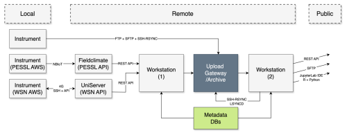
Figure 7 Example of a data stream from multiple networks and various databases (DBs), with the applications used in the production steps and the data store formats (bottom row) using scheduled scripts. The typical data stream is from local instruments to a remote server that provides public access.

A limitation of the current internet infrastructure is that an assigned network address cannot be reached from outside a private or mobile network without a virtual private network (VPN). By default, the data transfer can only be initiated from the local-access node to the remote storage node. VPN is available through some routers (e.g., model RUT240 and Teltonika services, Teltonika Network; Kaunas, Lithuania) or commercial remote desktop software (e.g., AnyDesk Software GmbH; Stuttgart, Germany). On occasions, both remote-access solutions are used to diagnose issues, transfer miscellaneous files, or reconfigure instruments from a remote office location.

3.5 Production levels

Participants and data systems produce many datasets and services. Most intermediate results are shared immediately and automatically for different uses. Production processes have production levels (some optional) to help keep track of data from collection to publication, as follows (Fig. 8).

• RAW. Data are recorded by instruments from multiple sources (e.g., campaign-deployed sensors, partners, third-party APIs).

• L0 (optional). Transcribed RAW data (i.e., to binary) with metadata attributes are typically aggregated to daily or monthly periods. This structured alternative to RAW data is intended to speed up data ingestion for subsequent data processing tasks, with variable vocabulary identical to the RAW input files.

• L1 (optional). Curated datasets have various processing (e.g., quality control, coordinate alignments, metadata standardization, translation of names and units according to conventions) but remain penultimate to L2.

• L2. Published or publication-ready datasets include metadata attributes, as the absolute minimum, such as title, source, keywords, references, authors, contributors, license, comments, history, and creation time.

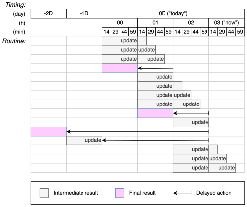
The production levels are collaboratively managed (Table 4). L0 products are typically scheduled automated routines (e.g., Figs. 8, 9, 2), with timing adjusted to recover if brief (2–28 h) data transmission delays occur between a local instrument source and the remote destination (Fig. 5). Beyond this, further interaction is needed (Appendix A1). L0 data are shared as input for diagnostics and other near-real-time analyses. Data products and intermediate results follow naming conventions given in Appendix B.

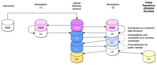
Figure 8 Pathways of data (from RAW to intermediate – L0, L1 – and publication – L2) with archiving at multiple stages. Data are shared (dark) and replicated (light).

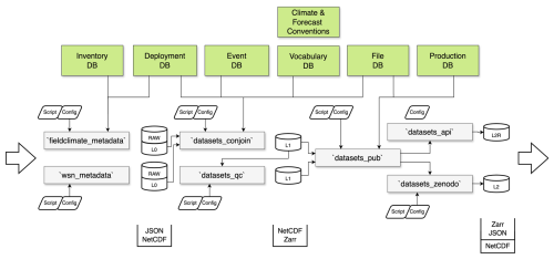
Figure 9 An example of a production line, the various databases (DBs) and applications used in the production steps, and the (bottom) data formats for data products for multiple uses. Scheduled scripts generate configurations that actuate the production line code during automation.

Richardson et al. (2018, PhenoCam network)Kotthaus et al. (2020, STRATfinder)Manninen et al. (2018)Vakkari et al. (2019, FMI code)Teschke and Lehmann (2017)Kayser et al. (2022, DWD code)Zeeman et al. (2022)Fenner et al. (2024a)Fenner et al. (2024b)Giles et al. (2019, AERONET)Feigel et al. (2024)VDI (2013, automated QC)Sulzer et al. (2022, online calibration and calculations)

Table 4 Example production lines used in the data management system.

3.6 Services

Web-based ICEs on workstations with common libraries and replicate programming environments are to develop code with immediate access to the data archive. The intent of this centrally managed ICE is to reduce interoperability issues arising between libraries and versions from individually maintained code environments. The common ICE has Python and R interfaces (JupyterLab), is modified upon request and documented (i.e., a GitHub repository), and, if needed, can be built by users with their own ICE (Appendix C2, Fig. C1).

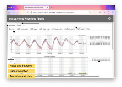
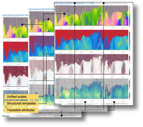
Visualization of data is implemented into internet-accessible applications (apps), developed and deployed by researchers using ICEs. The main evaluation of data processes, operational status, and availability relies on “quick-look” figures, automatically generated from RAW/L0/L1 data. These are integrated into interactive apps, or dashboards (Appendix C; notably C3). Data flows are monitored with respect to recorded data files and data within. The monitoring of computer system status, resource use, and alerts (“watchdog”) uses the open-source Nagios protocol and software.

APIs can enhance data access by providing dedicating handling of communication between computer programs and are used for many tasks. For some instrument subgroups, APIs are the main point of access to recorded data (e.g., a street-level automatic weather station network; Fig. C1). In turn, we provide access to curated data in near-real time to researchers and partners using APIs (Appendix C4). The Zenodo research data repository API helps simplify automated data management tasks for the publication of data (European Organization For Nuclear Research and OpenAIRE, 2013; Rettberg, 2018). The APIs use REST methods for communication (Appendix C4).

3.7 Operational costs

To help keep operating costs low, logical network design, careful configuration of data transfer tools, and automation are used. Semi-automated, central data collection allows multiple people to monitor instrument and network output in near-real time. The efficiency of incremental, compressed data transfer reduces data transfer volumes, allowing many systems (stations) to share one mobile phone data plan. User-level automation on local storage nodes (e.g., scheduled data transfer, local data housekeeping, and data transfer recovery after outages) reduces interference from running systems during maintenance (e.g., on-site swapping of storage cards). User-level automation on remote-access nodes and public-access nodes allows campaign data managers to control their data flow and allows multiple users to develop solutions for data monitoring, data exploration, and computation independently.

The virtual hardware is provided by the host (approx. EUR 500 to EUR 1000 per year) with a one-time purchase of data storage units (approx. EUR 40 000). The software tools are open-source, except for the remote-access software license (approx. EUR 250 per year). All tools need to be configured and programmed, for which the personnel costs include a data scientist as well as a researcher, a field technician, and research assistants for each campaign.

The benefits of near-real-time data access and cost savings must be weighed against costs (e.g., mobile phone network routers, data subscriptions, development time). Other operational costs involve the servers (e.g., configuration, maintenance of local- and remote-access nodes), storage (e.g., remote nodes, redundant backup systems) and public-access node workstations. Typically, local-access nodes are not modified during a campaign, so they require rigorous testing prior to deployment (Feigel et al., 2024). For our system, the remote-access, storage, and metadata database nodes consist of 10 servers using Windows, Linux, and OSX operating systems. All require frequent security updates to comply with institutional requirements and industry practice. Virtualization hardware, additional backup systems, and encryption certificates are provided institutionally. This data infrastructure can be expanded as required from multiple concurrent campaigns and projects.

4 Data governance

Most campaigns use data streams from partner instrumentation either directly or more typically from their data networks (e.g., weather service) or third-party networks (e.g., AERONET, PhenoCam network, ICOS, PANAME) (Giles et al., 2019; Richard et al., 2018; Haeffelin et al., 2023). Many of the latter are two-way contributions with campaign sensors also providing data to these networks. Data management is facilitated by assignment of roles and responsibilities. The roles are commonly shared or combined. Examples of different type of user roles of the system include (Figs. 2, 5, 7, 8; Table A2) the following.

• The principal investigator has executive responsibility for all scientific activities, campaigns, data, and peer-reviewed publications and priorities.

• The publication manager is responsible for the data publication process.

• The campaign manager is the lead for all aspects of a particular campaign (city).

• The data manager is the lead for data infrastructure supporting campaign teams.

• The researcher is responsible for a particular data production line or instrument group.

• The field operator is responsible for deployment and maintenance.

Many people take on data manager and researcher roles, with most at the end having the responsibility for publishing data. We should further recognize the responsibilities for (1) data science (i.e., scientific requirements, analysis, products), (2) data management (i.e., logical requirements, policies, workflow design, quality control), and (3) data infrastructure engineering (i.e., software and hardware architecture; software development; operations; performance management; end-to-end user, security, and network implementation). There are clear differences between these responsibilities, and having experts focus on each separately can arguably improve data system resilience and longevity. However, setting up teams of data experts is not common in soft-funded academic projects engaged in short-term collaborative observational campaigns, and responsibilities end up being carried by a few people (see Sect. 3.7).

Table 5 Glossary.

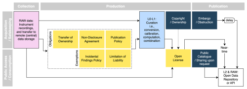
Figure 10 Pathways to making data publicly accessible require different data governance policies (yellow boxes) to be formalized early, allowing public access to be rapid and restrictions to be mitigated. Open access of collected data (RAW) is an option without such policies (bottom pathway), and embargoed release can be agreed with policies in place (center pathway), but the curation and analysis work (L0–L2) can involve intellectual ownership and personal interests that may otherwise lead to delays in open data publication (top pathway).

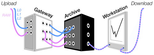
Figure 11 An info-graphic using a switchboard analogy is used to communicate where data are uploaded, where data can be downloaded, and where data streams (RAW and L0–L2 productions) are being managed, monitored, or modified.

Data governance needs to recognize the multiple participating members (e.g., campaign teams, project partners, land owners, external data providers, and data users) and their interests (e.g., contribution to outputs, liability limitations, expenses, funding agencies) and to provide open data using FAIR principles (i.e., findable, accessible, interoperable and reusable; Hassell et al., 2017). Thus, data governance covers (Fig. 10) the following.

• Formal agreements are for deploying instruments on a property or institutional platform (e.g., lattice mast) or location (e.g., observatory).

• Grant agreements (e.g., urbisphere data management policy) cover data ownership and grant compliance laws (e.g., European GDPR – General Data Protection Regulation 2016/679, FAIR, data security, and data retention).

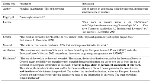
• L2 data are releases with a license (e.g., Creative Commons Attribution 4.0 International; CC BY 4.0), with terms of use adjusted in compliance with the license (Brettschneider et al., 2021). Various notices are included, e.g., license, creator, copyright, attribution, materials, disclaimer notice, and citation. The license notice is a machine-readable reference to the license, including a link or Uniform Resource Identifier (URI) to the full license text. The creator notice states the data authorship. The attribution notice includes a template to address attribution parties, e.g., to credit the primary funding agency. The disclaimer notice involves legal text regarding the limitation of liability and warranty. The material notice describes exactly what part of the work is covered by the license, such as data records, images, and text, but not the NetCDF database structure. Prior to release, the license and creator notice will not be included and a copyright notice is used instead (Table 6).

The data management agreements set requirements on how data will be stored and accessed, which must be communicated and made understandable to the individuals and associations involved (Fig. 11), regardless of their role in the organization of a campaign (Fig. 2, Table 1).

Table 6 Notices (e.g., disclaimers) accompanying data publications in the urbisphere project. Data published in near time have additional text (bold). The author list is updated at publication with an open license.

^* Additional wording is used for near-real-time publication (text in bold).

5 Conclusions

A resilient modular monitoring system for urban environments has been developed to allow rapid new deployments with changes in infrastructure and network technology, with a diverse set of field instruments being deployed during observation campaigns. The implementation primarily uses freely available software tools, established services for storing research data, and community-adopted conventions.

The system has to date been employed in several cities and different countries simultaneously. Our use cases involve not only research data products but also urban hydrometeorological services that reach the users – government officials, modeling teams, and the public – in near-real time through the implementation of FAIR principles.

Appendix A: Coordinate systems

In an urban deployment ensuring that a station is representative of the scale of interest is challenging, as is finding sites to deploy sensors. Often the place a sensor will be mounted is in a complex location, resulting in a need for a hierarchy of spatial coordinates (Fig. A3). For example, providing coordinates for a sensor mounted on a boom that extends off the edge of a roof is challenging yet required for accurate documentation (Fig. A). Similarly, further complications arise with sensors within buildings (Fig. A2). Fortunately, high-resolution geographic information systems are extremely common in cities, helping this process (e.g.,  Fenner et al., 2024b; Hertwig et al., 2024). Here, we use the follow coordinate systems.

• The Coordinate Reference System (CRS) is a commonly used global system, i.e., WGS84 or EPSG:4326. In some cases the UTM or a European reference system (i.e., ETRS89) can be useful alternatives, but their use in reporting must be explicitly specified in metadata.

• The vertical coordinate reference system (VRS) by default uses a global or regional system (e.g., European reference EVRS by EUREF; specifically the European Vertical Reference Frame, EVRF2007/EVRF2019, as it is integrated in the Global Navigation Satellite Systems, GNSS, and tied to the level of the Normaal Amsterdams Peil; Bundesamt für Kartographie und Geodäsie, 2023) and must be specified explicitly with a datum and coordinate system otherwise.

• In some cases, national reference systems may be used, when urbisphere observations need to be combined with local GIS data (e.g., spatial datasets provided by local authorities). In these cases, the respective ellipsoid and datum should also be specified.

• Urban heights. In urban deployments, all instrument configurations are linked to an “active surface” for which the height can be ambiguously interpreted as height above the ground (i.e., ground surface, topographic elevation) and height above a structure (e.g., a floor in a building, a roof terrace, a pavement level). Therefore, estimates of the altitude of the observation volume, as well as the altitude, height, and properties of the (nearest) urban feature and the surrounding topographic elevation, are documented in the metadata (Fig. A1b).

• Local coordinate systems. To help with the documentation of locations in the physical network, a local reference system was used. A fixed point on the active surface is defined as a station, from which offsets are measured in the field, such as the distance to the platform and any offsets from the platform to the observed volume (Fig. A1a). Any offset in the alignment with zenith and north are recorded as tilt and bearing (elevation and azimuth in CF standards, which are typically also recorded, e.g., by remote sensing systems and mobile platforms – compare Figs. A3d and e, respectively).

The information is stored in coordinates that are consistent with conventions and the hierarchical (physical) network (Table A1; see also Table 1). It is helpful to assume defaults, as particularly the vertical coordinates (altitude, topographic elevation of the ground level) need care to be determined and may be revised (Table A2).

Table A1 Coordinate attributes and the relationship between coordinate reference systems (i.e., station, using global CRS and VRS references; system, sensor, channel using local references) and metadata (i.e., conventions, standards, definitions, units).

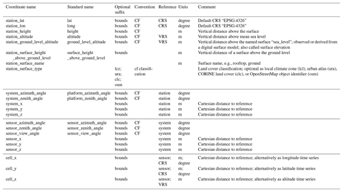
Table A2 Coordinate attributes and their meaning for metadata that are required, partially required, or required but set with a default value.

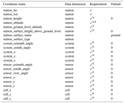
 ^a Required but can be derived. ^b Required, but a default value can be assumed if omitted.

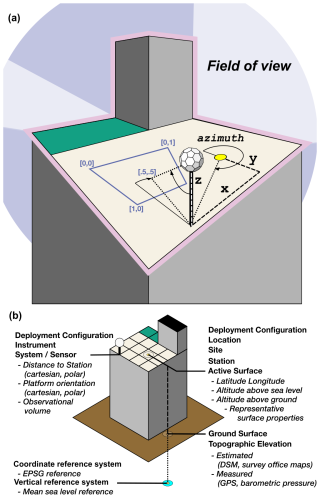
Figure A1 Deployment on a building roof with the relations between (a) a local station, platform, instrument, recorded image, and related coordinate systems in polar and Cartesian coordinates, as well as (b) local and global coordinate reference systems and features in the ordinance inventory and Earth observation.

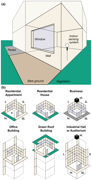
Figure A2 Indoor measurements of ambient temperature require uniquely different metadata compared to classical outdoor measurements, including additional coordinates for the orientation and features of the building, the room, the walls, and the adjacent space, as well as of objects that generate, transmit, transport, or intercept radiative heat.

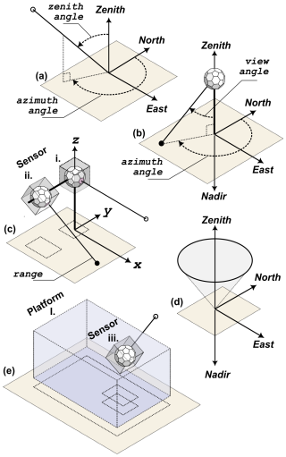
Figure A3 Metadata definitions for the relationships between platforms and instruments, as well as their coordinate systems.

A1 Time

Data management operates in close to real time or in short-interval batch acquisition (Fig. A4). All system clocks use UTC time (ideally), but if local time (without daylight saving) is locally essential the metadata include this information.

An accurate time convention is critical. The CF convention offers comprehensive and clearly defined options to describe and encode the start and end of intervals of time (or any other dimension). A basic option is to declare the relevant attributes of the “cell” value. For many of the data products, the data are “point” samples stored in their original sampling resolution. This is specified as an attribute to the variable (e.g., cell_method: "time: point"). Upon any aggregation, along the time dimension or any spatial dimension, the bounds can be (must be) declared and the cell_method attribute for those variables updated accordingly. The CF convention further reserves suffixes for aggregation to be added to the variable name, such as _mean and _maximum, to indicate that aggregation of data has occurred. Adding the time bounds technically implies adding a two-position virtual dimension to the data structure in order to store both the start and end of the interval coordinates along dimension time.

Besides the use of time bounds for aggregation periods in the data, metadata may also require intervals to be specified. The ISO8601 standard provides a detailed formatting description for the representation of periods as a machine-readable text. This notation works well in metadata records, including attributes in NetCDF data files, but the separator between the start and end time is defined as a forward slash character and is incompatible with use in file names (see Sect. B1).

Figure A4 The production schedule includes batch routines as well as sub-hourly and daily overlapping routines to recover data if short-term interruptions in networks occur (e.g., within the last 48 h).

Appendix B: Curation

B1 File names

To define locations, deployment configurations, and production stages, short-hand identifiers are used to structure both the metadata database relational features and the directories and files for data (Table B1).

Table B1 Naming convention for different types by production level with patterns and attributes.

• The project identifier is the organizational framework in which a data record is collected or computed. Many of the procedures and agreements depend on a formal separation of organizational units within the organizational network (see, e.g., Table 1).

• The production level (RAW, L0, L1, L2; see Sect. 3.5) represents the original source data that need to be archived in a different location than subsequent production stages.

• Instrument identifier vs. location identifier. The (re-)organization of data files by location can vastly improve the overview of the network, but a deployed configuration is typically unaware of its location and can only reliably provide instrument serial numbers as identification. The location short code is a CCNNNN format, which merges a two-character CC city code (optional) and a four-character NNNN station identifier. Station names are generally based on geographic neighborhood and not street names or property names to avoid referring to a company or trademark or disclosing exact locations, where privacy is affected. The station codes do not necessarily need to be unique; for example, stations FRCHEM and PACHEM operated simultaneously and are located in Freiburg (FR) and Paris (PA), respectively.

• Instrument classification. Most instruments can be configured to use a model identifier in their output file path and file header. In some cases, the output file format did not differ between instrument models (e.g., TOA5 data-logger files) and the output for a instrument group (e.g., data loggers) could be combined during subsequent production steps.

• Time. All file names include a time stamp or time bounds (in UTC), and in the case that large numbers of daily files are expected, additional sub-folders with year or date information facilitate manual file browsing.

Figure B1 Example of automatic quality control for AWS air temperature (ta; bottom panel) data to illustrate VDI 3786 (VDI, 2013) quality control indicators (vertical lines indicate bad quality; top panel).

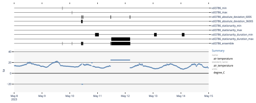
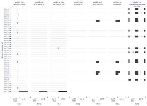
Figure B2 VDI 3786 (VDI, 2013) quality control indicators applied to the Freiburg AWS network (rows) during a storm (11 to 12 July 2023) for all variables (precipitation, pr_rate; air temperature, ta; relative humidity, hur; wind speed, ws; wind direction, wd; station pressure, plev; incoming shortwave (or global) radiation, rds) with quality flags shown: long – “bad”, short – missing.

The motivation for the use of definition rules for acronyms is not to be restrictive but to reserve acronyms for two-, three-, four-, and six-character uppercase acronyms for city, system group (Table 3), station identifier, and combined city–station identifier reference, respectively. We found the consistent use of those formats in metadata, communication, and publication helpful.

B2 Quality control

An automated assessment of typical meteorological variables was implemented using the Verein Deutscher Ingenieure (VDI) guidelines for meteorological observations (VDI, 2013). The guidelines provide threshold values for the range, rate of change (absolute deviation), and duration of steady state (stationarity duration) for a number of variables. The threshold values are specified for different averaging times. Testing the data with these threshold values determines for each data point if the quality is good, ambiguous, or poor. The procedure for change rate and steady-state calculations requires data before and after a data point to be available, and the computations involve repeated averaging at different time intervals, which incurs computational costs and complexity. Additional care is needed to ensure that the units between the data and threshold values match.

The output of the quality control is a new dataset with the same time dimension as the original data. The result can be summarized into an ensemble quality control indicator for specific variables, which can be useful for evaluation and masking data points before further use (Fig. B1). By combining all quality control output for a network of sensors and multiple variables, outliers and trends can be assessed (Fig. B2). The example describes a passing storm on the evening of 11 July 2023, registering (1) a rapid humidity change at most locations, (2) high variability in wind speed and/or wind direction at some locations depending on the orientation of the street canyon to the wind, (3) a possible malfunction in the precipitation sensor at FRLAND, (4) a possible time offset of the system at FRCHEM, and (5) an unspecified technical issue that affects the data delivery at FRTECH. The information should be considered indicative, as it can reveal both natural changes and technical problems, but can be further supported by spatial statistics (not implemented here) and field reports.

Appendix C: Services

C1 Computing environment

A system-wide copy of the Anaconda Python distribution (Anaconda Software Distribution, 2023) is installed on workstations in order to provide users with preconfigured Python and R environments. These environments are updated occasionally to introduce new features. The environments contain packages for scientific data analytics (e.g., functions for calculation, access to common data file formats) and access to the metadata DBs. Taking a pragmatic approach, we rely on Python libraries supported by the Numerical Foundation for Open Code and Useable Science (NumFOCUS, 2024). Libraries (xarray, pandas, numpy, scipy, and dask), plus useful extensions to NetCDF (e.g., data access: zarr, time conversion: cftime, unit conversion: cfunits) allow the produced NetCDF database files to be used in R and MATLAB ICEs as well as by dedicated NetCDF tools (e.g., NCO, CDO, Panoply), and vice versa.

C2 Online access

Each workstation functions as a web server, with certificate-based communication (HTTPS) using the host institution IT services and authentication for security. Web hosting has different domains for public and private access. The private domains have basic authentication with credentials entered in a web browser pop-up.

Apps are private not because of sensitive information but because of performance cost and operational risks linked to public access. Some experimental services have additional authentication (e.g., JupyterLab; Fig. C1). Although setting up web services requires system administrator changes to the workstation web proxy, researchers are free to manage their apps independently.

C3 Apps

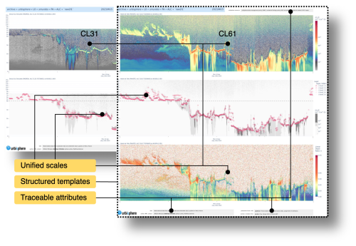
Web app templates, using open-source projects (e.g., shiny, panel), are modified to comply with publication guidelines, host institution policies, project policies, European law (e.g., terms of use statement), and other legal terms. The template header and footer information (e.g., location, contact, creation time, terms of use) identifies version status and formal reference if used (e.g., during talks). The templates are prepared using the plotly library, as it is available for multiple ICEs (e.g., R, Python).

Apps assist field operators, data managers, and researchers in diagnostics and early exploration.

• Diagnostics help monitor the network data stream (Fig. C2): overview of recently added or modified files, automated task status reports, interactive figures showing file count for individual systems in the past hour and days.

• Visualization of variables gives the operational status of dynamic processes (Fig. C3): templates combining metadata and data give automatic, distributed, provisional data for review of quality and availability (Figs. C4, C5, C6, and C7b).

• Outreach provides community-available near-real-time data (Fig. C7c; Feigel et al., 2024): can also be usable as a diagnostic tool.

C4 Data API

Methods to expose NetCDF4 data stores through a Representational State Transfer Application Programming Interface (REST API) are provided by libraries (zarr, xarray, fastapi, fsspec, xpublish; Fig. C7b). JSON output format, a widely supported text-based encoding format for data storage, is added to the API as local governments (e.g., city of Freiburg) require it for applications (e.g., urban planning, civil protection, disaster management, climate adaptation). However, as JSON is unsuitable for streaming large data queries (>10 MB), an alternative format is needed (i.e., Zarr). The JSON data output can be converted back to NetCDF (i.e., using xarray), ensuring that the output of the API from both Zarr and JSON can be used interchangeably.

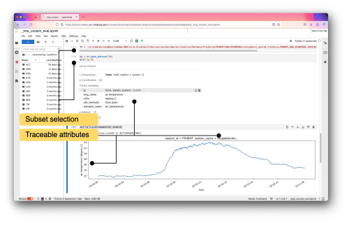
Figure C1 An example of a web browser data science environment and ICE (Jupyterlab; Kluyver et al., 2016) with simple code inspecting the data.

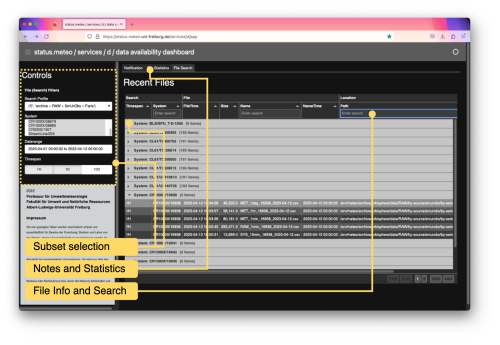
Figure C2 Dashboard app used to visualize the most recently changed files and folders by campaign (e.g., city).

Figure C3 As Fig. C2, but for the most recent data for inspection.

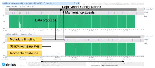
Figure C4 Example overview of available data as time against time of day, including metadata attributes to help identify attribution, location context, production information, and a timeline of events as known at the time of creation.

Figure C5 Near-time Doppler wind lidar (DWL) data used for diagnostics and data exploration.

Figure C6 As Fig. C5, but for the automatic lidar and ceilometer (ALC).

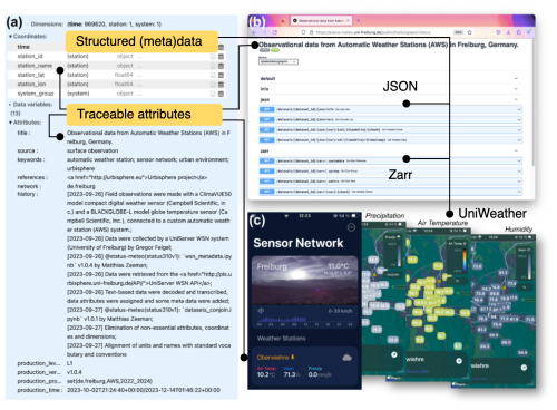
Figure C7 An example of (a) an AWS product summary, (b) a data API, and (c) the uniWeather phone app (Feigel et al., 2024) that use the same (meta)data dynamically. The map layers are copyright of Apple Inc., and the uniWeather app is copyright of Gregor Feigel.