Ultra-low-cost manual soil respiration chamber

Soil respiration measurement is important to assess natural carbon dioxide production. The closed-chamber technique allows relatively easy soil respiration monitoring. A planned spatially large-scale campaign incites us to implement our ultra-low-cost portative chamber. The chamber itself is entirely built from commercial parts with little, easy-to-perform, quick machining work. The resulting setup is an easy-to-operate, standalone, robust device. The used sensors are cost-effective yet accurate digital sensors that were successfully checked against some reference sensors. All of these characteristics made the described chamber accessible to build and use for a wide scientific and educational community. In this short note, we describe this simple device along with its sensors and apparent respiration quotient tip.

1 Background

On average, soil has nearly double the amount of carbon of the terrestrial atmosphere (Smith, 2012). Furthermore, it is one of the biggest generators of CO₂, and the frost-free soil generates nearly 10 times as much CO₂ as the whole amount of fossil fuels burned by humanity. Due to the increased microbial activity brought on by the increased soil temperature, this natural CO₂ production is increasing by around 0.1 % yr⁻¹ (Bond-Lamberty and Thomson, 2010). However, the further soil response to global warming is uncertain and arouses a large scientific interest (Todd-Brown et al., 2018; Jansson and Hofmockel, 2020; Soong et al., 2021; Bhatti et al., 2024)

In the context of global warming due to the increase in atmospheric greenhouse gas concentrations, such as CO₂, particular attention is given to soil respiration. There are several techniques and sub-techniques to achieve this goal. One of the most widespread techniques is the closed-chamber technique. This technique is about a century old (Bornemann, 1920), but it has been continuously improved and allows us to monitor more greenhouse gases (GHGs). Among closed chambers, we can distinguish automatic chambers and manual chambers. Each technique has its pros and cons (Savage and Davidson, 2003; Yao et al., 2009; Lee, 2018).

The automatic chambers allow it to operate automatically, which is a salvatory relief, allowing a relatively high operation rate, even during the night. However, the cost and complexity of these chambers prevents their large spread, leading to a relatively high incertitude when spatial variability is important.

Manually operated chambers rely on the same principle except that the chamber operations (closure and opening) are manual and require a human presence. This kind of chamber can hardly be used during the night, in rain, or in any meteorological condition that could make human presence exhausting. However, a punctual measurement can be done on a large spatial scale without any external power supply. Not only are these chambers portable, allowing the use of only one chamber in several locations, but the cost of the manually operated chambers is much less important compared to the automatic chambers. The lower this cost, the more important its duplication possibility, allowing a quick and large measurement campaign by a scientific group or for educational purposes.

This short note describes an ultra-low-cost (USD 200 for the basic configuration) and fast construction (1–2 weeks) chamber using ultra-low-cost, yet accurate, sensors (USD 20 to USD 100 for the basic sensors excluding oxygen sensors). The described chamber is built using only some commercially available parts requiring only a little machining work, which is so-called MacGyver science. (Hut et al., 2020). Also, to complete our knowledge about soil respiration, oxygen sensors were implemented, and their functioning will be described.

2 Materials and method

For the needs of large-scale spatial soil respiration measurements, a portable chamber with detachable stainless-steel collars to be placed in the soil was built. Cost-effective construction was sought but did not impair the quality of the measurements. As mentioned by numerous authors, the chamber needs to have its internal air mixed by a fan; proper sealing between the chamber and the soil is essential, along with a pressure equilibration device (Hutchinson and Mosier, 1981; Parkin and Venterea, 2010; Christiansen et al., 2011; Clough et al., 2013).

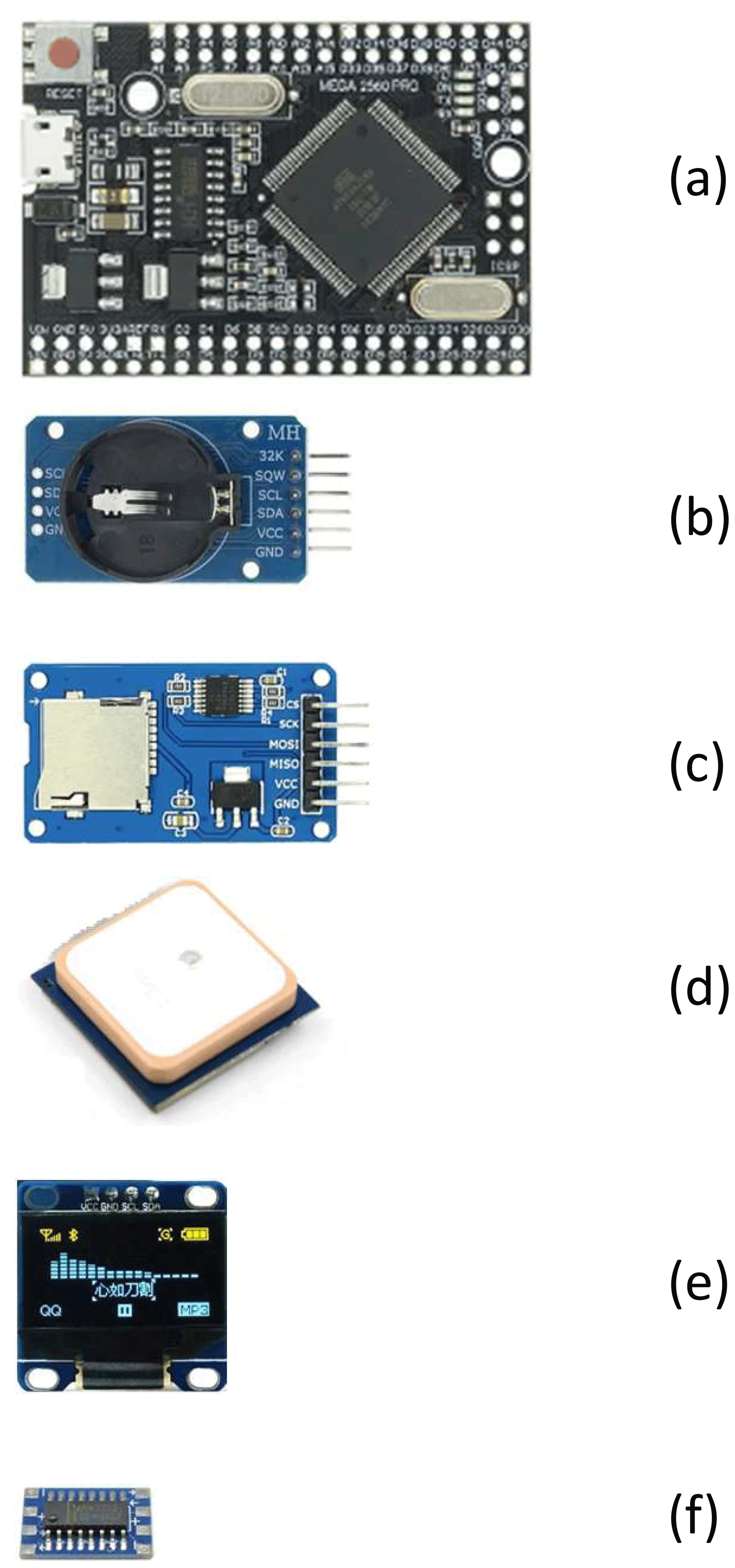
Figure 1 Data logger built with (a) Arduino Mega Pro, (b) RTC, (c) micro SD card reader, (d) GPS, (e) OLED display and (f) RS232 to TTL module.

2.1 Electronic modules composing the data logger

The manual soil respiration chamber described here employs a data logger made of commercial electronics modules for querying and logging information gathered by several sensors. The entire set of modules is housed in a handheld enclosure along with a GPS antenna. A basic UART TTL bus-attached GPS antenna was also incorporated because the same chamber is utilized in multiple locations to help track the precise location of the measurement (Fig. 1).

To read and log data from sensors, a data logger was built with a generic clone of an Arduino Mega Pro for its multiple digital buses (I²C, SPI and UART), its multiple hardware UART serial ports and its compactness. The real time is provided by a generic Real Time Clock module (RTC) powered by a precise DS3231 chip on an I2C bus from Dallas Semiconductor (Dallas, Texas, USA), owned nowadays by Analog Devices (Wilmington, Massachusetts, USA). A generic micro SD card reader on the SPI bus ensures data-saving ability. In the case of RS-232 bus use, a generic module based on an MAX3232 chip from Maxim Integrated (San Jose, California, USA), also owned by Analog Devices, converts the RS-232 level to the TTL level. A small fan (MC20100V3-Q01U-G99, 5 V, 0.33 W, 20 × 20 × 10 mm, MagLev from Sunon Electric Machine Industry Company Limited, Qianzhen, Kaohsiung District, Taiwan) fixed on a light and holed stainless-steel plate inside the cloche gently mixes internal air during the measurement cycle. The MagLev (magnetic levitation) life span is very long at 100 000 h, the rotating speed is relatively slow (11 000 RPM), the rated airflow is 1.2 CFM and the static pressure is less than 45 Pa.

A generic 0.96 in., two-color I²C OLED display allows us to indicate all useful information, such as the micro SD card state, GPS position reading, logger state, or battery charge level, along with current sensor readings and acquisition time (Fig. 2).

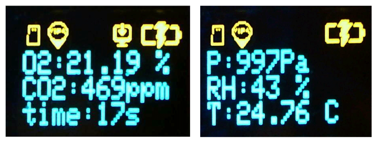
Figure 2 Small (0.96 in.), yet very readable, OLED display permuting screens with different useful information.

All electronics modules are housed inside a handheld enclosure (Fig. 3) that also contains a generic power bank module using two 18650 lithium-ion rechargeable batteries. The power bank filled with two generic batteries allows 12 h of uninterrupted operation. A USB socket and short cable allow charging the batteries using a generic USB charger but also establishing a link with the Arduino to program it or to withdraw the micro SD stored data without having to dismount the micro SD card. Three waterproof push buttons allow the operation of all electronics modules (power on/off, GPS coordinate memorization, internal fan operation, and launch/stop a measuring cycle). Two waterproof cable glands allow for safe passage of the sensors and fan cables.

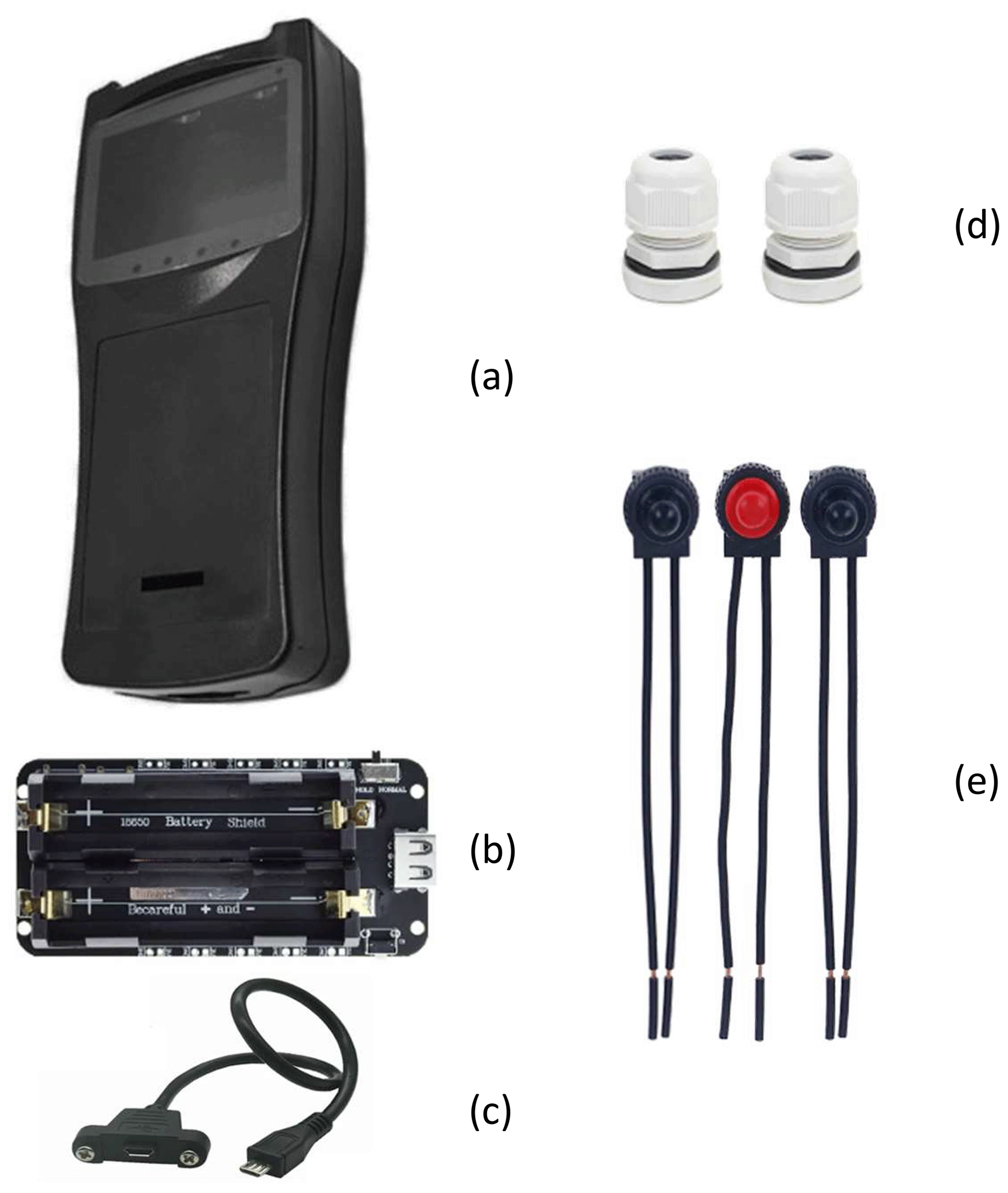
Figure 3 The enclosure is made from (a) a handheld enclosure, (c) a micro USB socket with a short cable, (b) a power bank, (d) two waterproof cable glands, and (e) three waterproof push buttons, i.e., one black self-locking on/off and two momentary (on)/off (one red, one black).

2.2 Body of the chamber

The body of the device (Fig. 4) is built around a sanitary stainless-steel Triclover (also called Triclamp) dome reducer (6–2 in.). The 2 in. opening is end-cap obturated and clamped with a 2 in. Triclover bracket and its Polytetrafluoroethylene (PTFE) joint. The 2 in. end-cap is pierced for one waterproof cable gland with 5 V power cable, I²C bus and eventually a UART bus cable. A second hole may be drilled for another cable gland that may be needed for an optional OXYBase oxygen sensor, and the third hole is for a small exhaust porous silencer used for the equilibration of internal air pressure with external air pressure during the measurement cycle. Two other small holes, tapered for M3 screws, are destined to hold two spacers on which the internal plateau is screwed. The second 6 in. opening is clamped during the operation on a stainless-steel collar previously placed into the soil at the chosen location. Again, a Triclover bracket and its PTFE joint, but 6 in. this time, ensures correct sealing between the chamber body and the collar. The collar itself is made from a 6 in. Triclover lathe-sharpened ferrule.

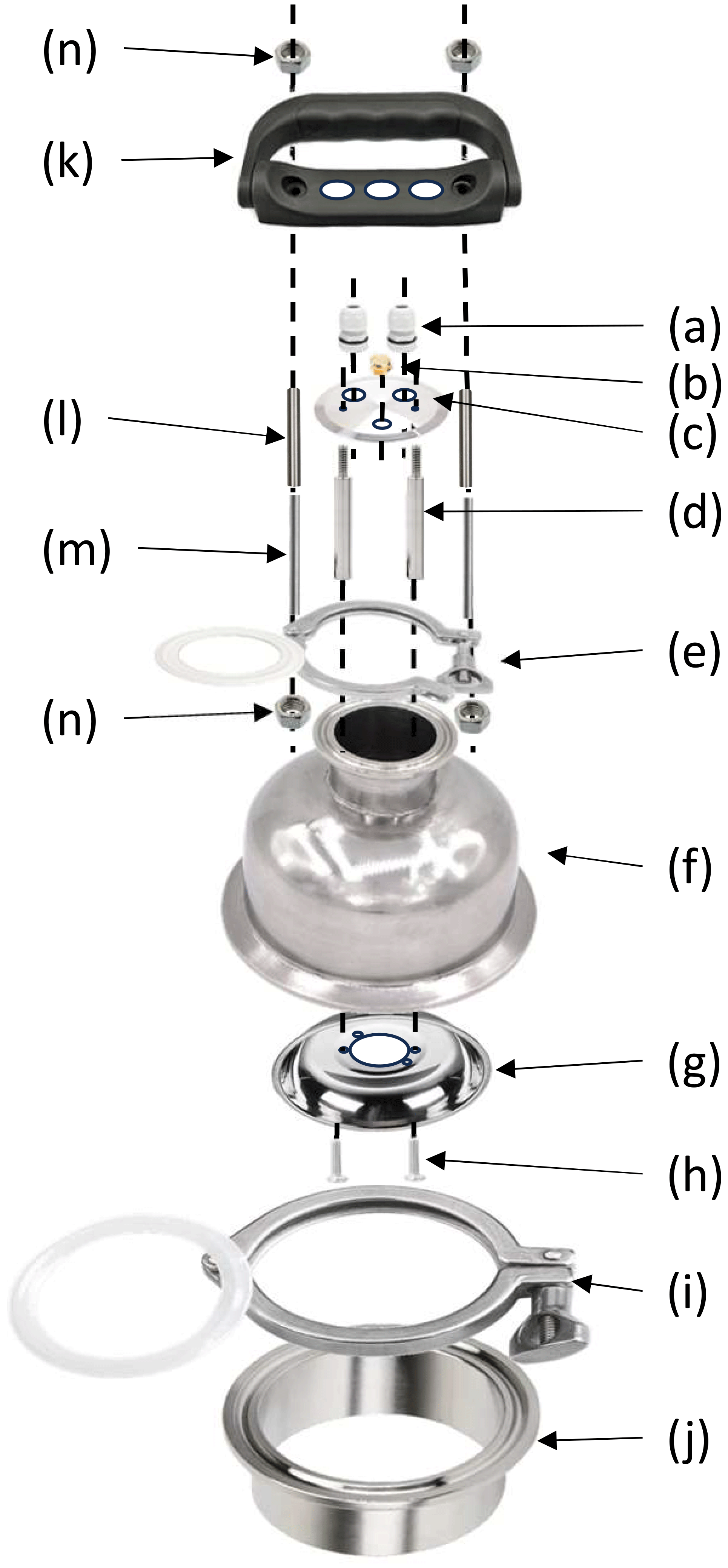
Figure 4 The body of the chamber is built with (a) two waterproof cable glands, (b) a small porous pneumatic silencer, (c) a 2 in. stainless-steel end cap, (d) two M3 spacers, (e) a 2 in. Triclover bracket with a PTFE joint, (f) a 6 in. to 2 in. Triclover reducer, (g) a small stainless-steel plate, (h) two M3 screws, (i) a 6 in. Triclover bracket with PTFE joint, (j) a 6 in. stainless-steel bottom-sharpened fitting, (k) a pierced plastic handle, and (l) a stainless-steel tube partially covering (m) the M4 threaded stainless-steel rod and (n) stainless-steel M4 nuts.

The 2 in. Triclover bracket studs were removed and replaced with a piece of stainless-steel M4 threaded rods partially covered with matching tube. On each end the rods are bolted, i.e., at the bottom to the bracket and on the top to the handle.

The handle was drilled to hold three push buttons on the upper side and the handheld enclosure on the bottom.

Figure 5 shows the overall finished setup.

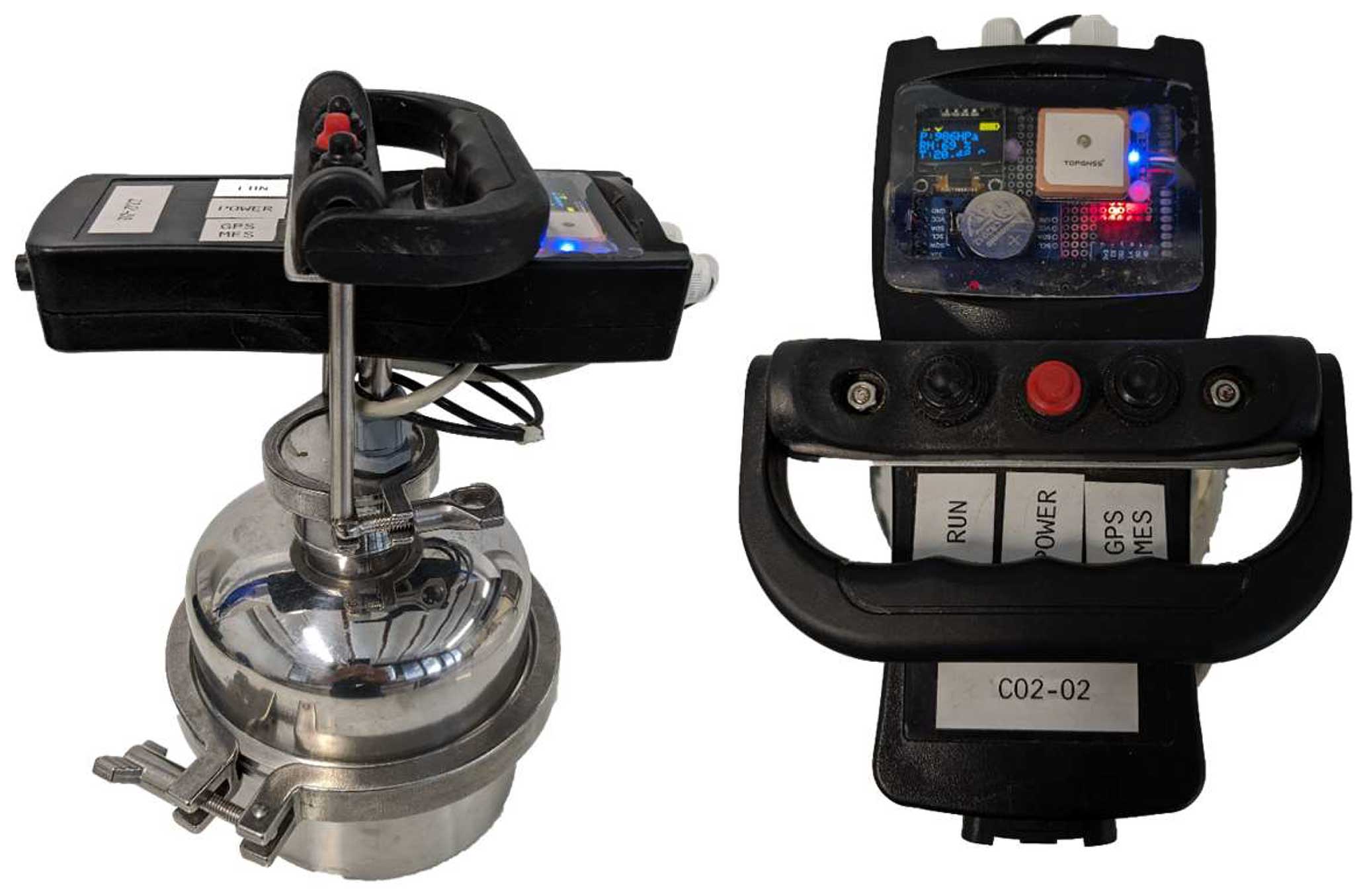
Figure 5 Side view of the assembled chamber positioned on the collar and top view of the chamber.

This chamber has an internal cloche volume (V = 1.65 dm³) to internal collar surface (S = 2.01 dm²) ratio of R = 0.82 dm. Of course when measurements are computed, the volume of air between the soil surface and the top of the collar has to be added to the cloche volume.

2.3 Embedded sensors and fan

The embedded sensors are the heart of the device. Nowadays, some miniaturized devices allow precise sensing of numerous physical quantities. The air pressure, temperature, and humidity can be precisely monitored by a minuscule BME280 sensor (Bosch Sensortec GmbH, Reutlingen, Germany).

Gas concentration monitoring can be achieved with any small and accurate-enough sensor. Several techniques are available, such as semiconductor, electrochemical or optical. We do not embed a methane (CH₄) sensor, but this is a possibility using a semiconductor sensor (Riddick et al., 2020; Bastviken et al., 2020; Furst et al., 2021).

For CO₂ concentration monitoring, non-dispersive infrared (NDIR) sensors are currently used (Hodgkinson et al., 2013; Dinh et al., 2016). They are relatively cost effective, small, and accurate enough. In addition to CO₂, some other gases, such as carbon monoxide, can be monitored with the NDIR sensors (Diharja et al., 2019). Other miniaturized sensors can be used for CO₂, but we found the NDIR-based sensors have the best quality-to-cost ratio for CO₂ measurement. Indeed, photoacoustic sensors, such as PASCO2V1 from Infineon, are small and digital, with the same accuracy as NDIR, and they are relatively cheap with a long lifetime (10 years) but are slow (τ₆₃ < 90 s), which implies a slow sampling (minimum 5 s, typical 60 s) that is not adapted for rapidly evolving concentration monitoring. Electrochemical sensors, such as MG811 from Gravity, are small and relatively cheap, but their accuracy is 100 ppm only, they are analog, and as with most electrochemical sensors their stability and lifetime are relatively limited. Among NDIR sensors, the most significant criterion used for sensor selection was its accuracy, then its rapidity and finally its price.

Precise oxygen depletion measurement is challenging as the main atmospheric oxygen concentration (20.9 %) is relatively high compared to the concentration variations in the closed chamber. When the CO₂ concentration can be multiplied by 5 after a few minutes inside a closed chamber, the oxygen concentration decreases only by barely a few percent of the initial concentration. Following this, the sensor dedicated to the oxygen concentration measurement should be particularly accurate and stable. For this reason, we chose to work with optical sensors such as LuminOx and OXYBase. The LuminOx (SST Sensing Ltd., 5 Hagmill Crescent, Shawhead Industrial Estate, Coatbridge, UK) is based on non-depleting luminescence technology, and the OXYBase (PreSens-Precision Sensing GmbH, Regensburg, Germany) is based on quenching luminescence. The absolute accuracy, resolution and response time of the OXYbase sensor is better than that of the LuminOx sensor. The OXYbase sensor costs over 6 times as much as LumiOx as the cost is substantially nonlinear with accuracy. We then have to choose based on our goal. The oxygen sensors are by far the most expensive sensors on this device (USD 100–650). Oxygen depletion measurement is interesting and brings new insights into the respiration process (Turcu et al., 2005; Helm et al., 2021); however, their use is still optional.

Table 1 The mentioned measured parameters are pressure (P), temperature (T), relative air humidity (RH), carbon dioxide concentration (CO₂) and oxygen concentration (O₂).

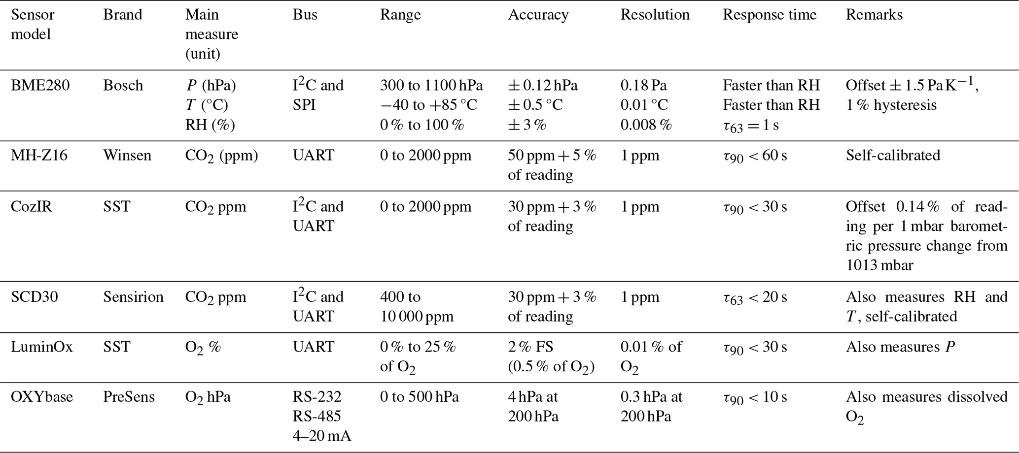
The models used and some of the existing sensor specifications are summarized in Table 1. Notice that the provided specifications apply to room temperature and pressure ranges. Some of the sensors have several possible configurations, providing different measurement units, for example. However, in Table 1, for the sake of clarity only one of the possible configurations is given.

Figure 6 shows the used sensors and fan embedded under the cloche.

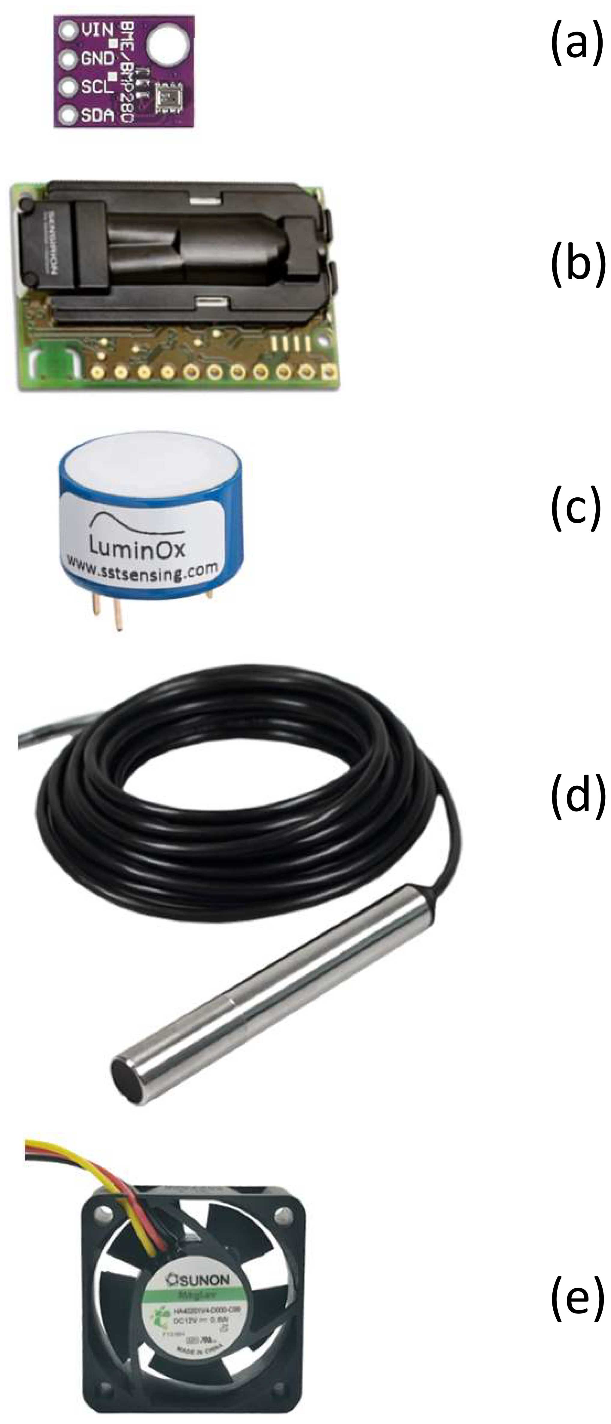
Figure 6 Used sensors and fan: (a) BME280, (P, T, and RH); (b) SCD30 (CO₂) ©Sensirion CH, all rights reserved; (c) LuminOx (O₂) ©SST UK all rights reserved; (d) OXYBase (O₂) ©PreSens D, all rights reserved; and (e) Maglev fan.

All gas-analyzing sensors are digital and placed under a cloche on a dedicated prototype printed circuit board (PCB) held by the fan. The embedded fan gently mixes the air entrapped under a closed cloche to homogenize it as thoroughly as possible without provoking pressure pulsations that may affect measured effluxes (Le Dantec et al., 1999; Koskinen et al., 2014). The semi-spherical shape of the cloche helps to prevent poorly mixed areas (Livingston and Hutchinson, 1995).

BME280 is used to measure air pressure, temperature, and humidity. Air humidity measurements are necessary to deduce the dry molar fraction of the gases of interest (LI-COR, 2024) or to calculate the soil evaporation rate (Zawilski, 2022). SCD30 (Sensirion AG, Stäfa, Switzerland) is a cost-effective NDIR sensor that provides CO₂ concentration, air temperature and air humidity. However, these two last parameters are already provided by BME280 with better accuracy. Both oxygen sensors, LuminOx and OXYBase, were tested, but only one should be used at a time. LuminOx also measures the air pressure. However, once again, BME280 provides air pressure with very good precision that may be used for both sensors.

3 Sensor tests

Embedded sensors such as SCD30 for CO₂ and LuminOx or OXYBase for O₂ concentration measurement were truly checked, if possible, by cross-calibration with a reference sensor or performing a reference experience (respiration).

3.1 SCD30 cross test

Before using the SCD30 sensor for CO₂ monitoring, it was tested by comparison with the high-precision optical-feedback cavity-enhanced absorption spectroscopy (OF-CEAS) Li-7810 from LI-COR (LI-COR Biosciences, Nebraska, USA) for 3 months using six chambers. To avoid any difference between measurements due to the air-leading tubes, we installed SCD30 and Li-840A (LI-COR Biosciences, Nebraska, USA) close to the Li-7810 in the same external circuit. Figure 7 shows all the measurements of Li-7810 versus SCD30. A linear regression of these measurements shows a good correspondence with a 1.08 slope and a small offset of less than 27 ppm with a rather high correlation coefficient (R² = 0.98). It is worth noting that SCD30 exhibits much better correspondence with Li-7810 than our flow-through LI-840A Infra-Red Gas Analyzer (IRGA), which is not self-calibrated and probably quickly deserves a deep cleaning despite the air filter presence (Fig. 8).

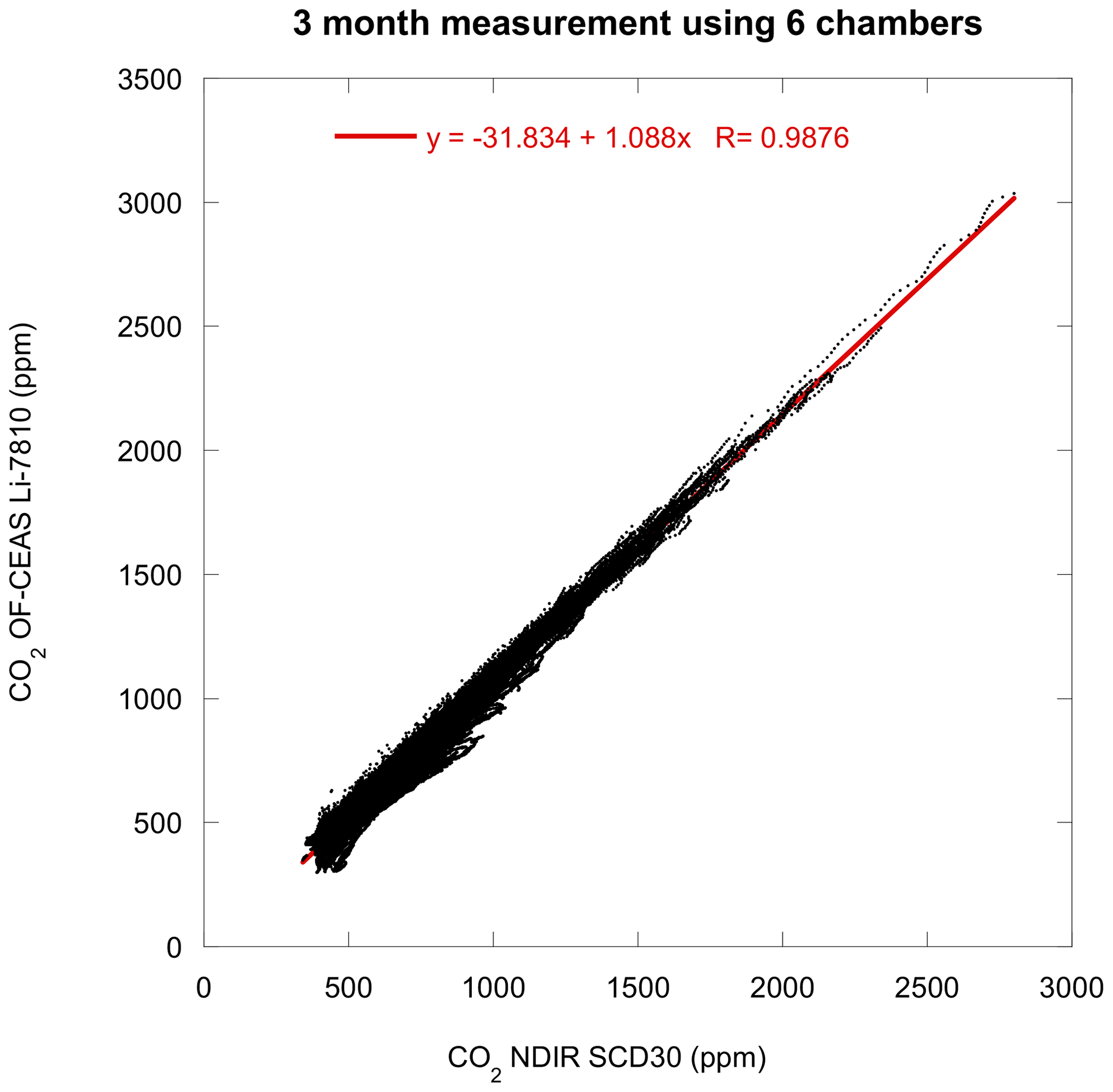
Figure 7 OF-CEAS Li-7810 measurements versus NDIR SCD30 measurements during a 3 month campaign conducted with six chambers. The solid red line represents a linear regression.

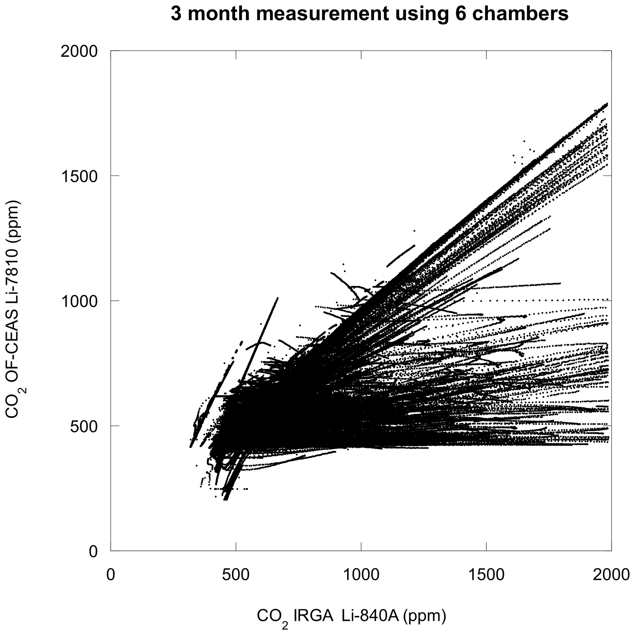
Figure 8 OF-CEAS Li-7810 measurements versus IRGA Li-840A measurements during 3 months. The Li-840A derived during the test presents measured CO₂ saturation for 2000 ppm due to the analog output configuration.

The calculated $F_{{\mathrm{CO}}_{\mathrm{2}}}$ from SCD30 data were compared to the $F_{{\mathrm{CO}}_{\mathrm{2}}}$ from Li-7810 data.

To create comparison between SCD30 and Li-7810 data we use the concentration variation and calling it $F_{{\mathrm{CO}}_{\mathrm{2}}}$; however, it is not exactly a usual flux expression. Usually, we are talking about carbon grams per square meter and per second and not about carbon dioxide parts per million per second, but between both expressions there is only a multiplicative factor that depends on delimited soil surface, chamber and emerged collar volume, and air temperature and pressure. All these quantities are the same for SCD30 as they are for Li-7810. As we will see later, correct chamber operation should be based on carbon dioxide variation during chamber closure, which is easy to monitor using $F_{{\mathrm{CO}}_{\mathrm{2}}}$ in parts per million per second.

Figure 9 Computed fluxes from SCD30 and Li-7810 data compared.

The qualitative accord of the calculated “fluxes” is rather good even if for this calculation a constant closure duration was used (3 min). For a quantitative accord check, an integration of all calculated fluxes is compared in Fig. 10.

Figure 10 Accumulated fluxes from SCD30 and Li-7810 data.

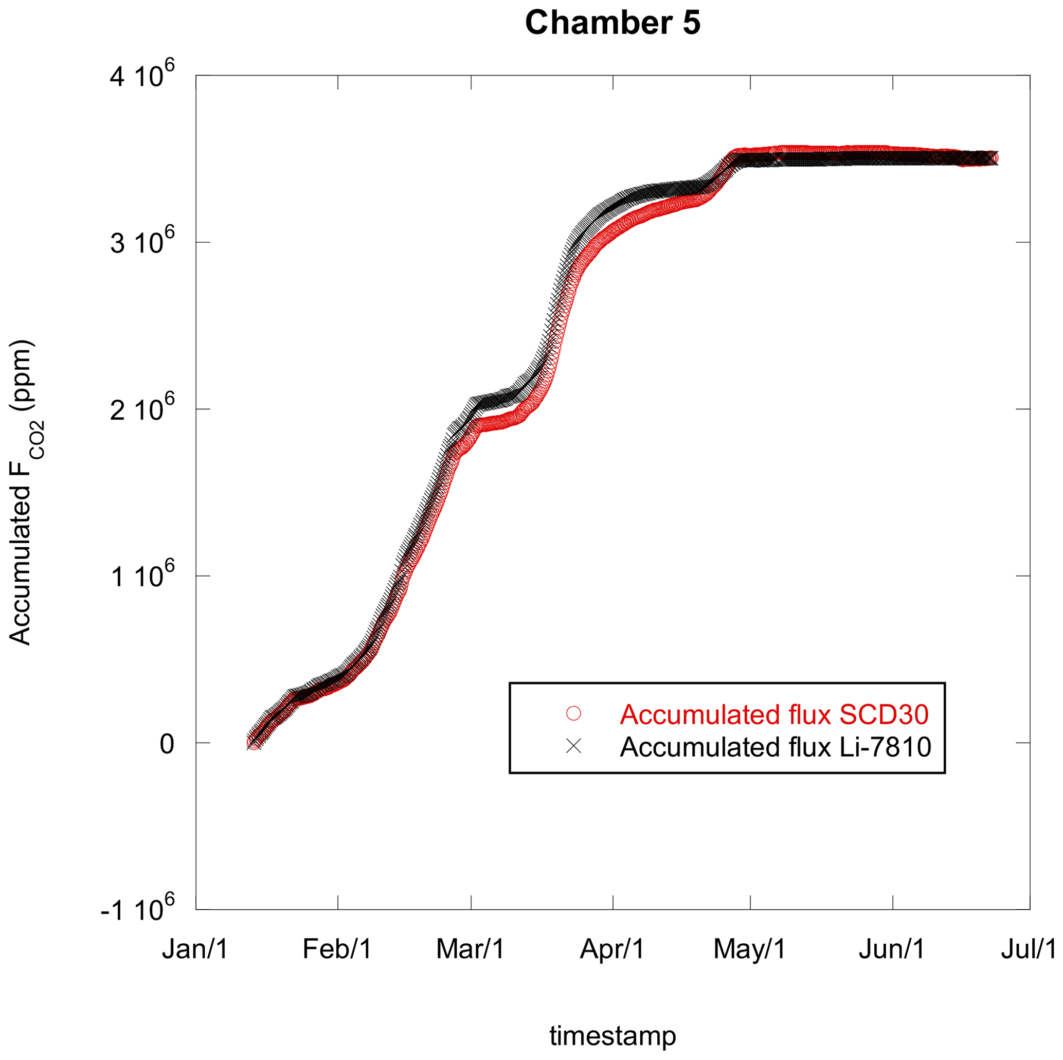
The accumulated fluxes match well except when the measured fluxes are very small. In this case, as shown further check, a longer chamber closure duration may improve the SCD30 measurements quality. However, even with a constant closure duration, the SCD30 and Li-7810 measured fluxes are rather close.

As suggested by one referee we performed some additional checks. The SCD30 sensor was enclosed in an enclosure constantly vented with a CO₂ gas mixture of 1000 ppm concentration for 6 h. We take and log SCD30 measurements every 2 s, obtaining about 11 000 data points (CO₂ concentration versus time). Using obtained data to simulate chamber closure during 1 min, we took 30 consecutive points intervals. With the selected data, using linear regression, we calculated the “apparent flux” and logged it into a file with a timestamp corresponding to the beginning of each selected time interval. We do it again with a data set starting from the second point of the 11 000 point data set up to the end of the data set less the interval duration. Thus, we have an “apparent flux” calculated on 11 000−30 points. The same job is done for 2 min closure duration, which is 60 selected data points. We then obtained a second file with 11 000−60 data points with a timestamp and “apparent flux” for 2 min chamber closure and so on up to the 20 min chamber closure duration. In the end, we have 20 files with apparent fluxes calculated for one 1 min chamber closure duration of up to 20 min with a 1 min step. Thus, we were able to perform statistical analysis on the fluxes computed during the 6 h with increasingly variable closure duration. Figure 11 presents the minimum, the maximum, and the mean values of the computed fluxes during 6 h versus the closure length. The real flux is null and the apparent computed fluxes reflect the measurement errors.

Figure 11 Computed fluxes minimal, maximal and mean values versus closure duration.

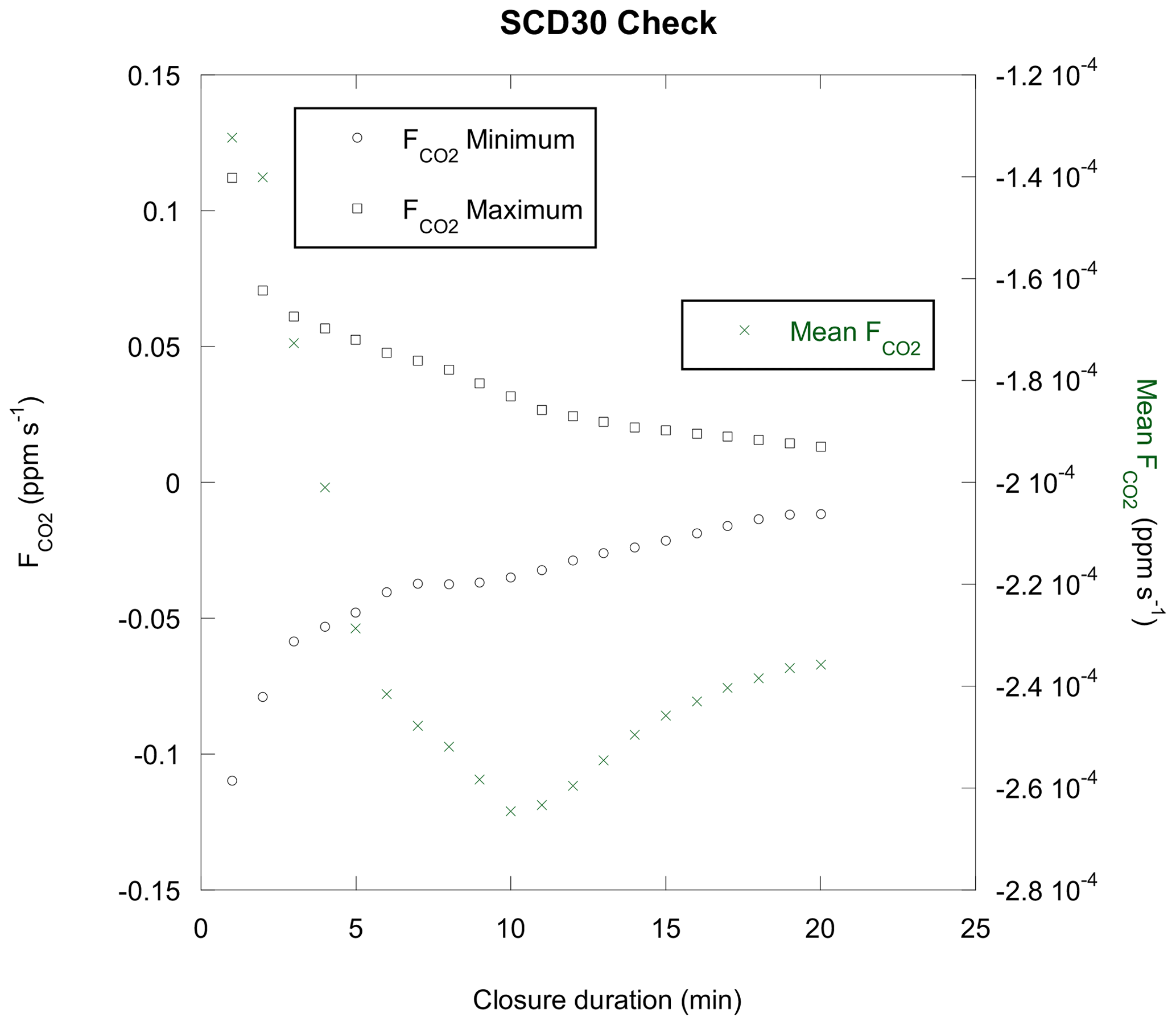
The standard deviations of the computed fluxes are summarized in the Fig. 12.

Figure 12 The standard deviation of the computed fluxes versus closure length.

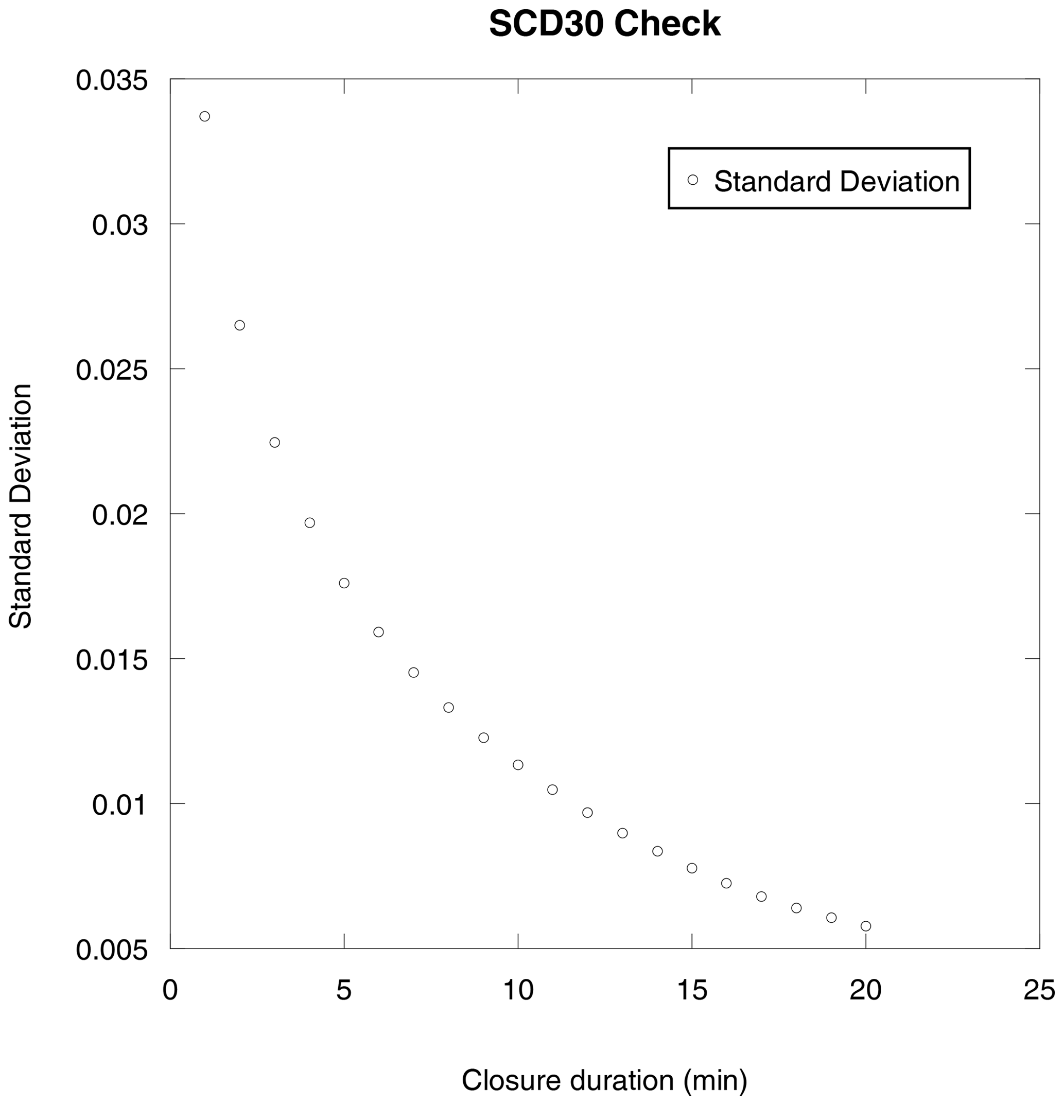
As expected, the longer the closure is, the smaller the minimum and maximum fluxes errors are with the smallest standard deviation. We can note that the mean flux is always negative and that its evolution is not monotone but displays an extremum at about 10 min of closure duration. Whatever the closure duration is, the mean apparent flux is still of the order of 2 × 10⁻⁴ ppm s⁻¹, which is rather small. Punctually, the computed flux may be relatively important in distorting small flux measurements, especially if a short closure is adopted. The operator has to decide when the measurement should be stopped, and one of the most important criteria is the overall measured gas concentration variation amplitude.

A good air analyzer is always preferable to a small (or even minuscule) analyzer. However, small analyzers can be embedded under the cloche when big analyzers can only function outside of the chamber, which induces some other problems such as air-leading tube disturbances and internal condensation. In addition, the price difference between an Li-840A and an SCD30 is about 160-fold, and between an Li-7820 and an SCD30 the difference is about 1300-fold.

However, for some GHGs, such as N₂O, a miniaturized, precise-enough analyzer does not exist. A variant of the described chamber, designed for an external multi-gas Fourier-transform infrared spectroscopy (FTIR) GT5000 Terra analyzer (Gasmet Technologies Oy, Vantaa, Finland), was built. In this case, only the BMP280 and the fan were embedded under the cloche, and the data were transferred to a laptop PC via Bluetooth. Two fittings on the top of the chamber were added for air-leading tubes (in and out). A detailed discussion about the problems with external analyzers will be presented elsewhere.

Arduino programming is relatively simple. All I²C bus-attached devices have available libraries and programming assistance widely available on the web. UART-bus-based sensor communication is relatively easy to establish. The GPS also has numerous libraries that can be used, as they generally use the NMEA 0183 protocol.

3.2 LuminOx and OXYBase cross-tests

To test the oxygen sensors, we performed a comparison between LuminOx and OXYBase sensors performing an apparent respiration quotient (ARQ) measurement test with both sensors at the same time. To test the ARQ measurement, an animal contained in a closed space would be very helpful. However, any experimentation including an animal is strictly regulated by law. These restrictions do not concern volunteer humans, and one of us accepted being briefly closed in a vinery with a clean, pressurized tank of 22 hl volume (2.2 m³). The CO₂ and O₂ evolutions were monitored by a battery-powered data logger reading all available sensors at the same time.

As expected, the CO₂ evolution with time is nearly linear.

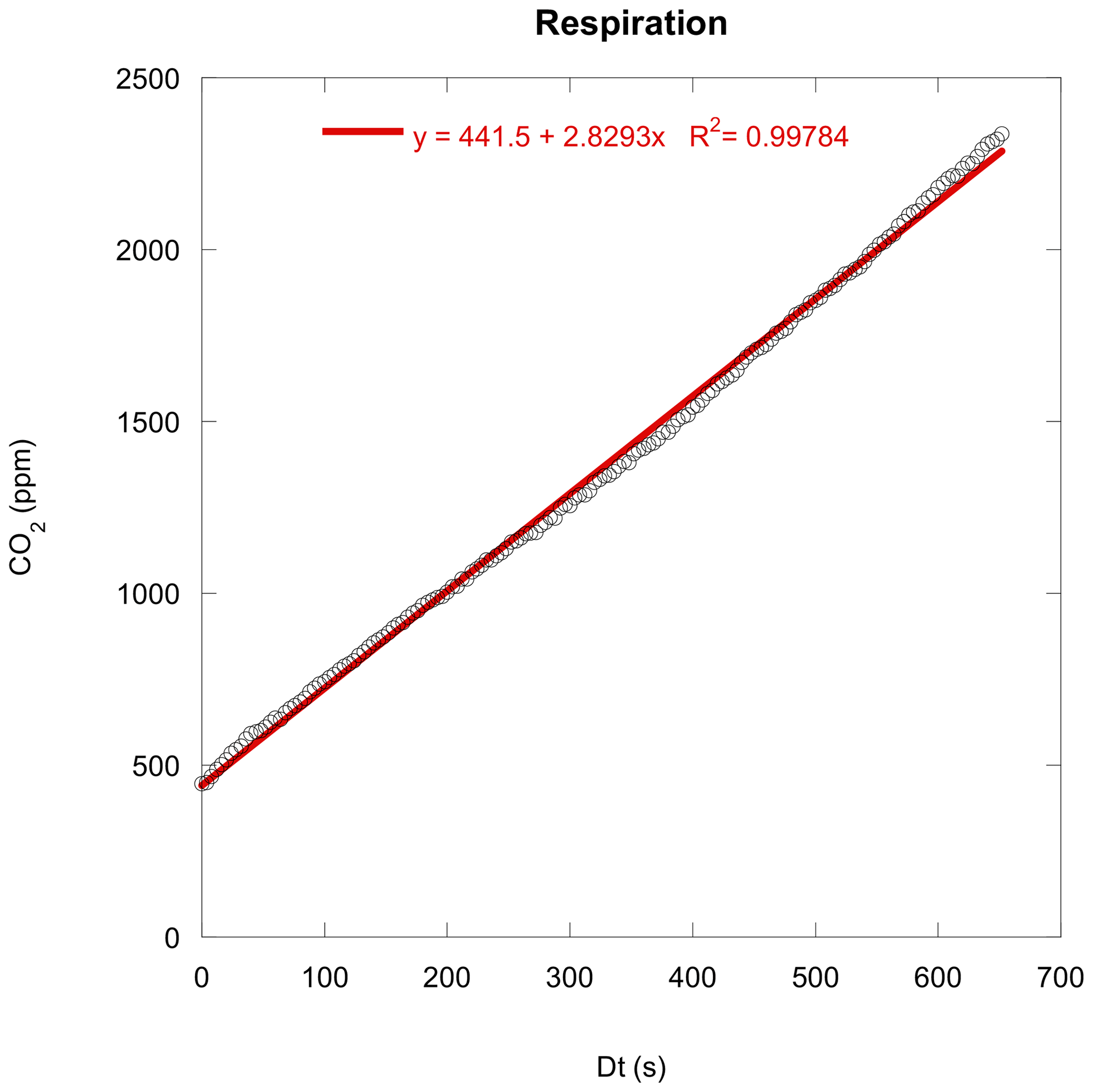
Figure 13 Measured CO₂ evolution in a tank with a breathing human inside. The solid red line represents a linear regression.

The O₂ evolution measured by LuminOx and OXYBase was close with a small offset and relatively matching slope.

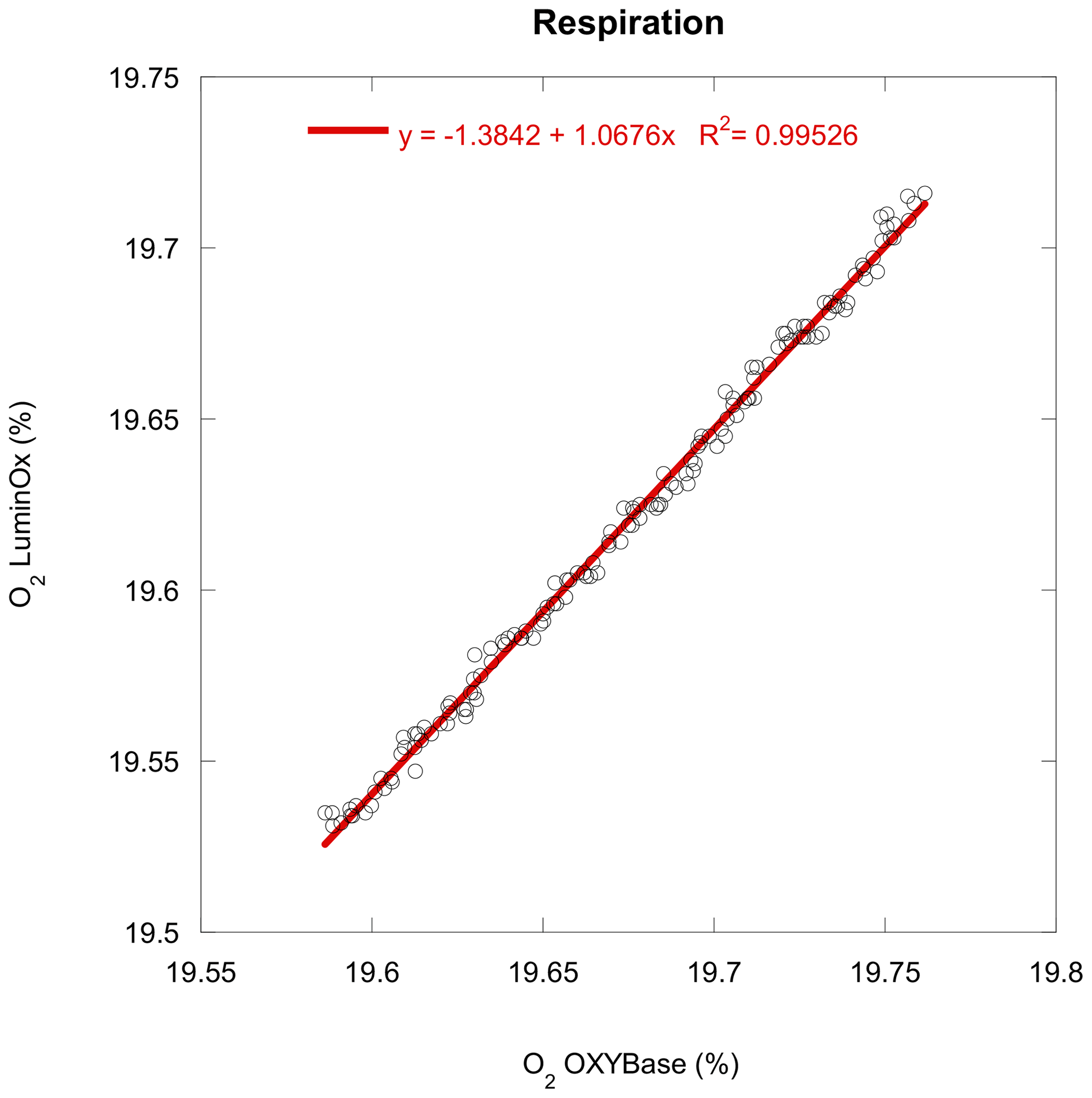
Figure 14 Measured O₂ part with LuminOx versus O₂ measured with OXYBase during the respiration experience. The solid red line represents a linear regression.

The ARQ calculation, using a linear regression explained in Sect. 5 and determined with OXYBase's measurements, is 0.97 when the ARQ determined with LuminOx's measurements is 0.90. Both sensors allow a relatively accurate ARQ calculation.

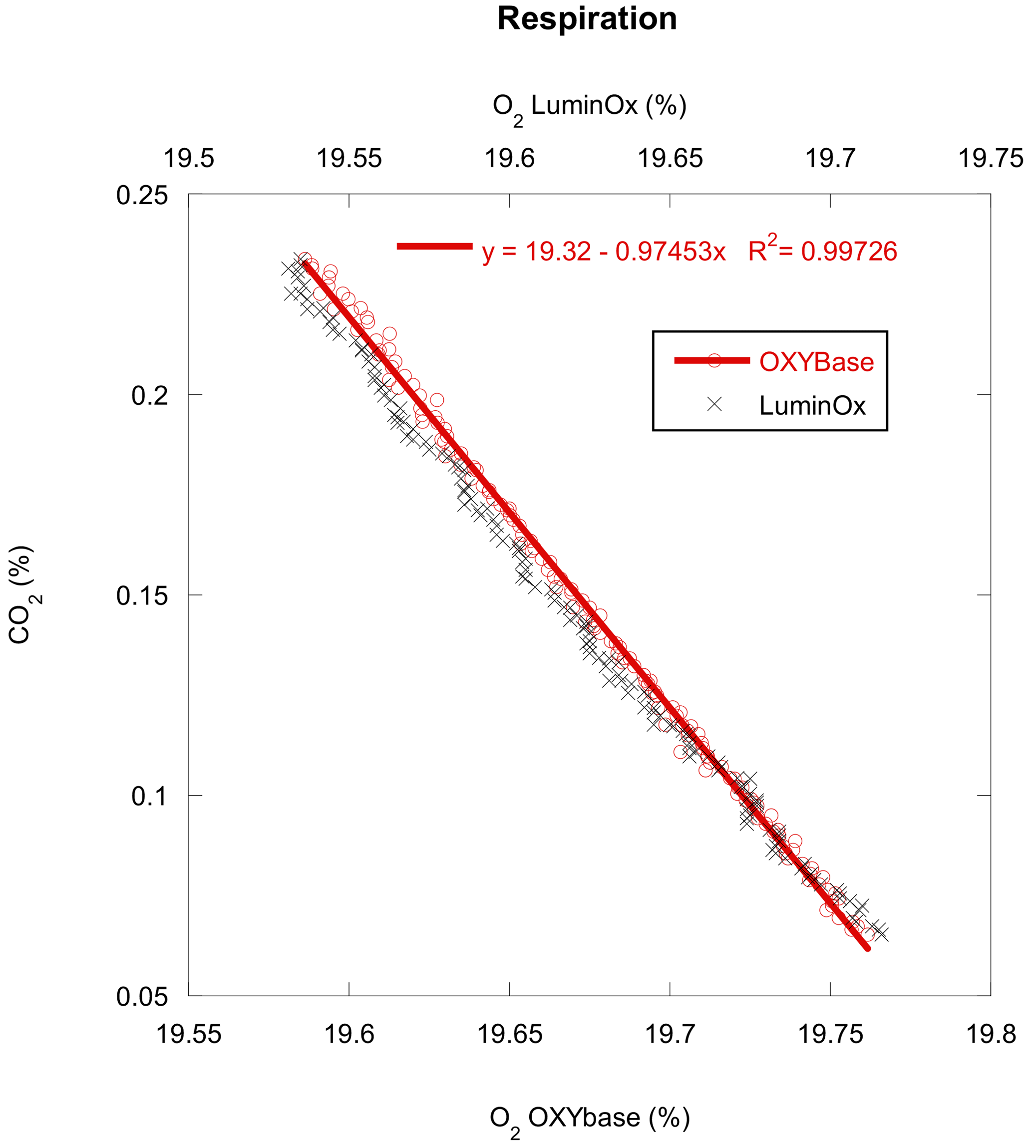
Figure 15 CO₂ measurements versus O₂ measurements done by OXYBase (lower abscissa) and O₂ measurements done by LulminOx (upper abscissa). The solid red line represents a linear regression of CO₂ versus O₂ measured by OXYBase.

4 Typical results

A typical measurement with a closed chamber technique displays CO₂ rising and O₂ decaying with time. Historically, the effluxes or influxes were calculated using a linear regression on the initial data. However, several authors have shown that linear regression can lead to a severely biased calculation (Kutzbach et al., 2007; Silva et al., 2015), but it is beyond the scope of this paper to discuss it here. As an illustration, we use the “exponential rise” regression, also called “asymptotic regression”. Figure 16 displays a typical carbon dioxide accumulation measured with a chamber positioned on its collar pressed into the soil.

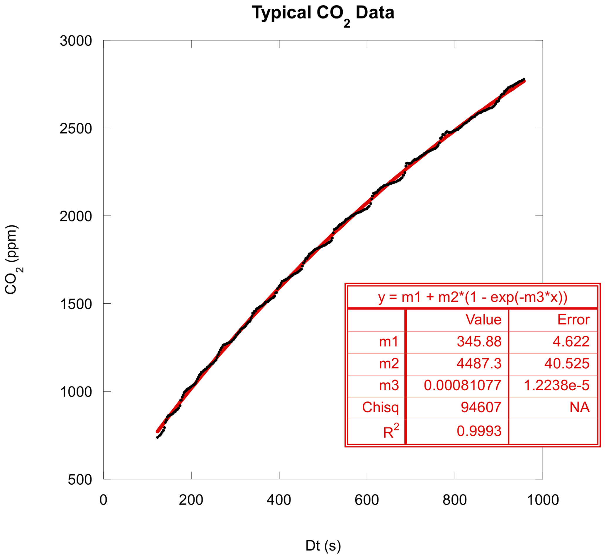
Figure 16 Typical CO₂ measurements in the chamber. The solid red line represents an asymptotic regression (fit).

The calculated CO₂ efflux $F_{{\mathrm{CO}}_{\mathrm{2}}}$ would then be

$$\begin{array}{}\text{(1)}& F_{{\mathrm{CO}}_{\mathrm{2}}}=m\mathrm{2}\times m\mathrm{3}\times R,\end{array}$$

with m2 and m3 being the curve regression constants calculated using a plot of CO₂ concentration versus closing time (Fig. 16) and R being the actual volume-to-surface ratio. The measured asymptotic concentration is given by the sum m1+m2 and represents the CO₂ concentration in the superior soil layer (0.5 % here).

A similar calculation could be conducted on the O₂ concentration to determine the oxygen influx.

Figure 17 displays a typical O₂ measurement taken at the same time as the CO₂ concentration in Fig. 16.

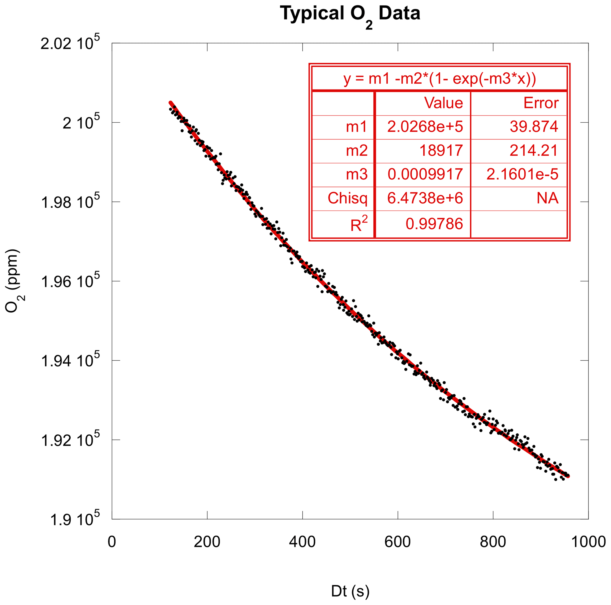
Figure 17 Oxygen concentration measurement versus time. The solid red line represents an asymptotic regression.

Similar to $F_{{\mathrm{CO}}_{\mathrm{2}}}$ calculations, the corresponding oxygen influx $F_{{\mathrm{O}}_{\mathrm{2}}}$calculation would be

$$\begin{array}{}\text{(2)}& F_{{\mathrm{O}}_{\mathrm{2}}}=m\mathrm{2}\times m\mathrm{3}\times R,\end{array}$$

with m2 and m3 being the constants deduced from an asymptotic regression of the plot of O₂ concentration versus time and R being the same volume-to-surface ratio as for the $F_{{\mathrm{CO}}_{\mathrm{2}}}$ calculation in Eq. 1. Always similar to the asymptotic CO₂ concentration, the measured asymptotic O₂ concentration is given by the difference m1−m2 and represents the O₂ concentration in the superior soil layer (18.4 % here).

5 Apparent respiration quotient circulation

To determine the apparent respiration quotient (ARQ), by definition we can proceed with a quotient of $F_{{\mathrm{CO}}_{\mathrm{2}}}$ and $F_{{\mathrm{O}}_{\mathrm{2}}}$ formation.

$$\begin{array}{}\text{(3)}& \mathrm{ARQ}={\displaystyle \frac{F_{{\mathrm{CO}}_{\mathrm{2}}}}{F_{{\mathrm{O}}_{\mathrm{2}}}}}\end{array}$$

This quotient comes from the definition of the ARQ (CO₂ flux divided by O₂ influx).

In the reported typical measurements, when using this quotient ARQ = 0.194.

However, this calculation accumulates uncertainties in nonlinear regressions used for both $F_{{\mathrm{CO}}_{\mathrm{2}}}$ and$F_{{\mathrm{O}}_{\mathrm{2}}}$ determinations.

Another simple way to calculate ARQ would be to use CO₂ concentration versus O₂ concentration and then a linear regression to give direct ARQ. Indeed, if we suppose that ARQ is constant during the time of the chamber closure, we can write the following:

$$\begin{array}{}\text{(4)}& \mathrm{ARQ}={\displaystyle \frac{\frac{\mathrm{d}{\mathrm{CO}}_{\mathrm{2}}}{\mathrm{d}t}}{-\frac{\mathrm{d}{\mathrm{O}}_{\mathrm{2}}}{\mathrm{d}t}}}.\end{array}$$

Then

$$\begin{array}{}\text{(5)}& {\displaystyle \frac{\mathrm{d}{\mathrm{CO}}_{\mathrm{2}}}{\mathrm{d}t}}=-\mathrm{ARQ}\times {\displaystyle \frac{\mathrm{d}{\mathrm{O}}_{\mathrm{2}}}{\mathrm{d}t}}.\end{array}$$

By integration

$$\begin{array}{}\text{(6)}& {\mathrm{CO}}_{\mathrm{2}}\left(t\right)=-\mathrm{ARQ}\times {\mathrm{O}}_{\mathrm{2}}\left(t\right)+{\mathrm{C}}_{\mathrm{0}}.\end{array}$$

With C₀ being a constant, we can write the following:

$$\begin{array}{}\text{(7)}& C_{\mathrm{0}}=\mathrm{ARQ}\times {\mathrm{O}}_{\mathrm{2}}(t=\mathrm{0})+{\mathrm{CO}}_{\mathrm{2}}(t=\mathrm{0}).\end{array}$$

Figure 18 displays the typical CO₂ and O₂ measurements already shown in the previous figures, but this time the CO₂ concentration is plotted versus the O₂ concentration. A linear regression provides simple ARQ determination.

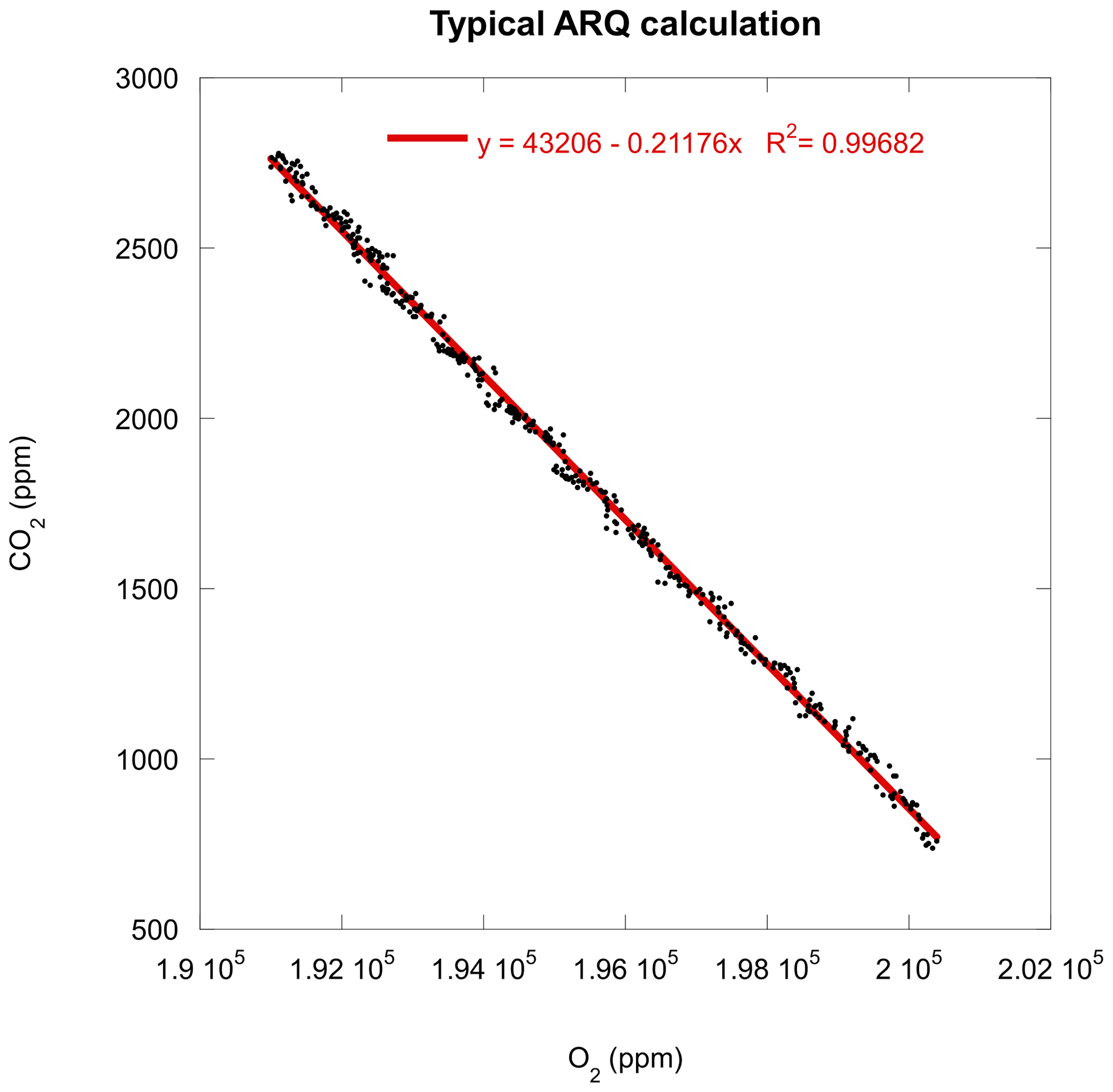
Figure 18 CO₂ concentrations versus O₂ concentrations. The solid red line represents a linear regression.

We can note that the ARQ provided by the linear regression of CO₂ concentrations versus O₂ concentrations (ARQ = 0.212) is slightly different from the ARQ calculated using the $F_{{\mathrm{CO}}_{\mathrm{2}}}$ and $F_{{\mathrm{O}}_{\mathrm{2}}}$ quotients (8.5 % difference). For ARQ determination, we suggest using a CO₂ concentration versus O₂ concentration plot and a linear regression, as it does not accumulate successive nonlinear regression uncertainties. We may also note that the measurements done with this chamber using low-cost sensors provide an excellent confidence level R², matching the theoretical linear and asymptotic regression.

An expected ARQ would be close to 1, as for respiration the same amount of O₂ is absorbed as the quantity of CO₂ released. However, this does not account for the fact that the soil may capture and store a consequent amount of the produced CO₂ (Sánchez-Cañete et al., 2018).

6 Conclusion

The importance of the soil's most significant natural CO₂ production measurement does not have to be proved. For this purpose, an ultra-low-cost portable chamber was built and is described in this note with the hope of helping our scientific community develop their own devices. The described chamber uses only commercial parts with little mechanical work. All used sensors are digital and cost-effective yet accurate enough to allow measurements with excellent confidence level R² when regressed to adequate linear and nonlinear laws. The described chamber is easy to build and easy to operate, allowing a wide range of users to work with it.