the Creative Commons Attribution 4.0 License.
the Creative Commons Attribution 4.0 License.
 | 26 Apr 2024
A distributed-temperature-sensing-based soil temperature profiler
Bart Schilperoort
César Jiménez Rodríguez
Bas van de Wiel
Miriam Coenders-Gerrits
Storage change in heat in the soil is one of the main components of the energy balance and is essential in studying the land–atmosphere heat exchange. However, its measurement proves to be difficult due to (vertical) soil heterogeneity and sensors easily disturbing the soil.
Improvements in the precision and resolution of distributed temperature sensing (DTS) equipment has resulted in its widespread use in geoscientific studies. Multiple studies have shown the added value of spatially distributed measurements of soil temperature and soil heat flux. However, due to the spatial resolution of DTS measurements (∼30 cm), soil temperature measurements with DTS have generally been restricted to (horizontal) spatially distributed measurements. This paper presents a device which allows high-resolution measurements of (vertical) soil temperature profiles by making use of a 3D-printed screw-like structure.
A 50 cm tall probe is created from segments manufactured with fused-filament 3D printing and has a helical groove to guide and protect a fiber-optic (FO) cable. This configuration increases the effective DTS measurement resolution and will inhibit preferential flow along the probe. The probe was tested in the field, where the results were in agreement with the reference sensors. The high vertical resolution of the DTS-measured soil temperature allowed determination of the thermal diffusivity of the soil at a resolution of 2.5 cm, many times better than what is feasible using discrete probes.
A future improvement in the design could be the use of integrated reference temperature probes, which would remove the need for DTS calibration baths. This could, in turn, support making the probes “plug and play” into the shelf instruments without the need to splice cables or experience in DTS setup design. The design can also support the integration of an electrical conductor into the probe and allow heat tracer experiments to derive both the heat capacity and the thermal conductivity over depth at high resolution.
- Article
(6477 KB) - Full-text XML
- BibTeX
- EndNote


The exchange of heat between the atmosphere and the land surface is one of the main components of the local energy balance. This heat exchange takes place at the surface but is driven by the temperature gradient between the surface and the soil deeper down. The process is strongly affected by soil cover (vegetation), soil type, and the hydraulic and thermal properties of the soil.
In order to study land–atmosphere heat exchange, knowledge of the surface skin temperature is important (Holtslag and De Bruin, 1988; Heusinkveld et al., 2004). Unfortunately, from an observational perspective, measuring this skin temperature is very challenging (Van de Wiel et al., 2003). With traditional sensors the upper soil is easily disturbed, as the observation should be done as close to the surface as possible. Moreover, the soil near the surface can be strongly heterogeneous due to larger organic matter content as compared to deeper soil layers. As measurements of the skin temperature are made at finite depth, it can thus be questioned how representative these are.
Alternatively, modeling approaches can be followed in order to infer the skin temperature from deeper soil temperatures: as the surface temperature varies with the diurnal rhythm, many analyses focus on the amplitude damping (van Wijk and de Vries, 1963; Van de Wiel et al., 2003), phase shifts, or harmonics (Verhoef, 2004; Heusinkveld et al., 2004; van der Tol, 2012; van der Linden et al., 2022) to model the propagation of heat through the soil. With these methods, the soil temperature and heat flux measured at certain depths are interpolated and extrapolated to infer an entire profile, or the heat flux and temperature at the surface. However, these methods are sensitive to the parameterization of, among others, how easily heat moves through the soil, i.e., the soil thermal diffusivity (Xie et al., 2019). For determining the soil thermal diffusivity, the soil temperature of at least three depths is required (although if one assumes the soil to be homogeneous over depth, two can suffice). This means that high-resolution profiles of thermal diffusivity require an even higher density of temperature measurements. Besides, the vertical variability in organic content and water content will make the diffusivity height dependent.
Not only are the soil temperature models sensitive to the parameterization, great care has to be taken in the placement of the sensors themselves. Near-surface temperatures can be very heterogeneous due to differences in soil cover or vegetation height. Deeper down this is less of an issue, as any surface differences will smooth out due to lateral diffusion (Eppelbaum et al., 2014). Note that small changes in sensor depth estimates may result in large temperature changes, particularly near the surface, where gradients are expected to be large. Thus, exact determination of the depth at which the sensors are located is very important, as uncertainties in this will propagate through the analysis (Dong et al., 2016). Some soil sensors already take this into account by affixing multiple temperature sensors to a solid structure which is placed into the soil, ensuring that the relative spacing is accurate down to the millimeter.
In recent years distributed temperature sensing (DTS) has become more prominent in studies of soil temperature and properties. Many of these studies have aimed to measure the spatial distribution of soil moisture, either with passive measurements combined with the soil properties (Steele-Dunne et al., 2010) or by actively heating the fiber-optic (FO) cable to gain more information on soil thermodynamic properties (Sayde et al., 2010; Shehata et al., 2020; Wu et al., 2021) Other studies focused on measuring the spatial distribution of the soil heat flux or surface heat flux (Jansen et al., 2011; Dong et al., 2016; Bense et al., 2016). In nearly all these studies the fiber-optic cables were placed horizontally in the soil, sometimes with a specially designed plow. Even then, horizontal cable placements will have some uncertainty, and small errors in the placement depth strongly affect results (Steele-Dunne et al., 2010). However, simply placing a cable vertically has no use due to the spatial resolution of DTS measurements, which is 0.25 m at its best. To overcome this, the cable can be placed in a fixed-coil shape (Vogt et al., 2010; Briggs et al., 2012; Hilgersom et al., 2016; Saito et al., 2018; Schilperoort et al., 2020; Wu et al., 2020). Affixing the cable to a coil effectively increases the vertical resolution, and this can ensure that the distance between each measurement point is both fixed and more accurate than with separate sensors or cables. In Saito et al. (2018), the soil temperature profile in both the top layer of the soil and snow covering the soil was measured using fiber-optic cable wrapped around a large-diameter PVC tube. However, these large-diameter PVC tubes can be challenging to install without disturbing the soil to a great extent.
To this end we designed a DTS-based soil temperature probe that can be placed into an hand-auger-dug hole in the soil, using a fiber-optic cable as the screw thread. A screw-shaped soil sensor already exists in the form of Campbell Scientific's SoilVue 10 sensor. However, while this sensor can measure the soil temperature and soil moisture over depth, it does so at either six or nine discrete depths. With a coiled fiber-optic cable, DTS can measure the soil temperature on a continuum and at higher resolution. In this technical note we discuss the design of the probe and how to build it, and we test the probe in the field with a comparison to reference sensors. We present the temperature profiles and derived diffusivity profiles that can be measured using the probe, as compared to standard discrete sensors. Lastly, we will discuss the limitations of the design and give an outlook to improvements and future use cases.
2.1 Probe design
The concept behind the design (Fig. 1) is twofold: place more optical fiber in a smaller space for a higher resolution and create a helical screw thread. When the fiber-optic (FO) cable that is used for the probe has a large diameter (e.g., 6 mm), the cable itself can act like the screw thread to ensure good contact with the soil. This is required to get a representative temperature measurement and will also prevent water from flowing straight down along the tube. Such a probe could be constructed by 3D printing or by adding a spiral groove in, e.g., a PVC pipe with a lathe. However, note that a screw thread design cannot be used for soils that experience a large amount of shrinkage (e.g., clayey soil), as this would prevent good contact with the soil.
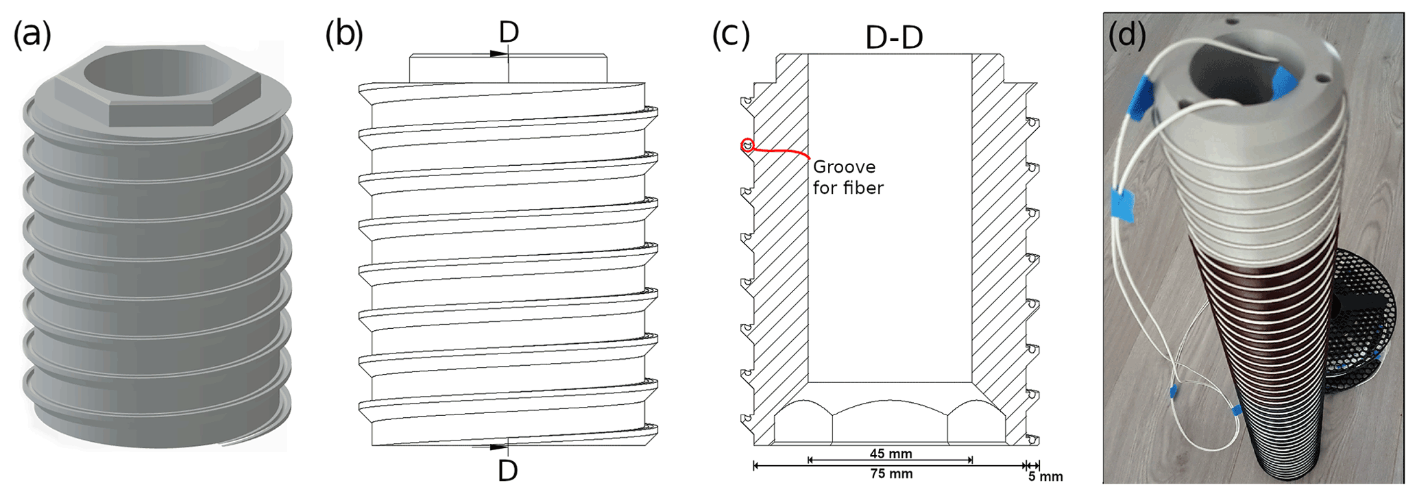
Figure 1A 3D render (a), side view (b), and vertical cross-section (c) of a segment of the DTS probe. A photo of the probe with all elements assembled is shown in panel (d).
Additionally, a cable with a low heat capacity and low thermal conductivity is also required to avoid disturbing the temperature profile of the soil (Fig. 2). As cables with a large diameter often contain metal, which is highly conductive, we chose to use a thin fiber-optic cable as an alternative. However, with smaller-diameter cables, the “screw thread” would not protrude out from the core as far. This could cause insufficient contact with the soil. A second issue is that smaller-diameter cables have less protection for the fiber, which increases the chance of damage during installation.
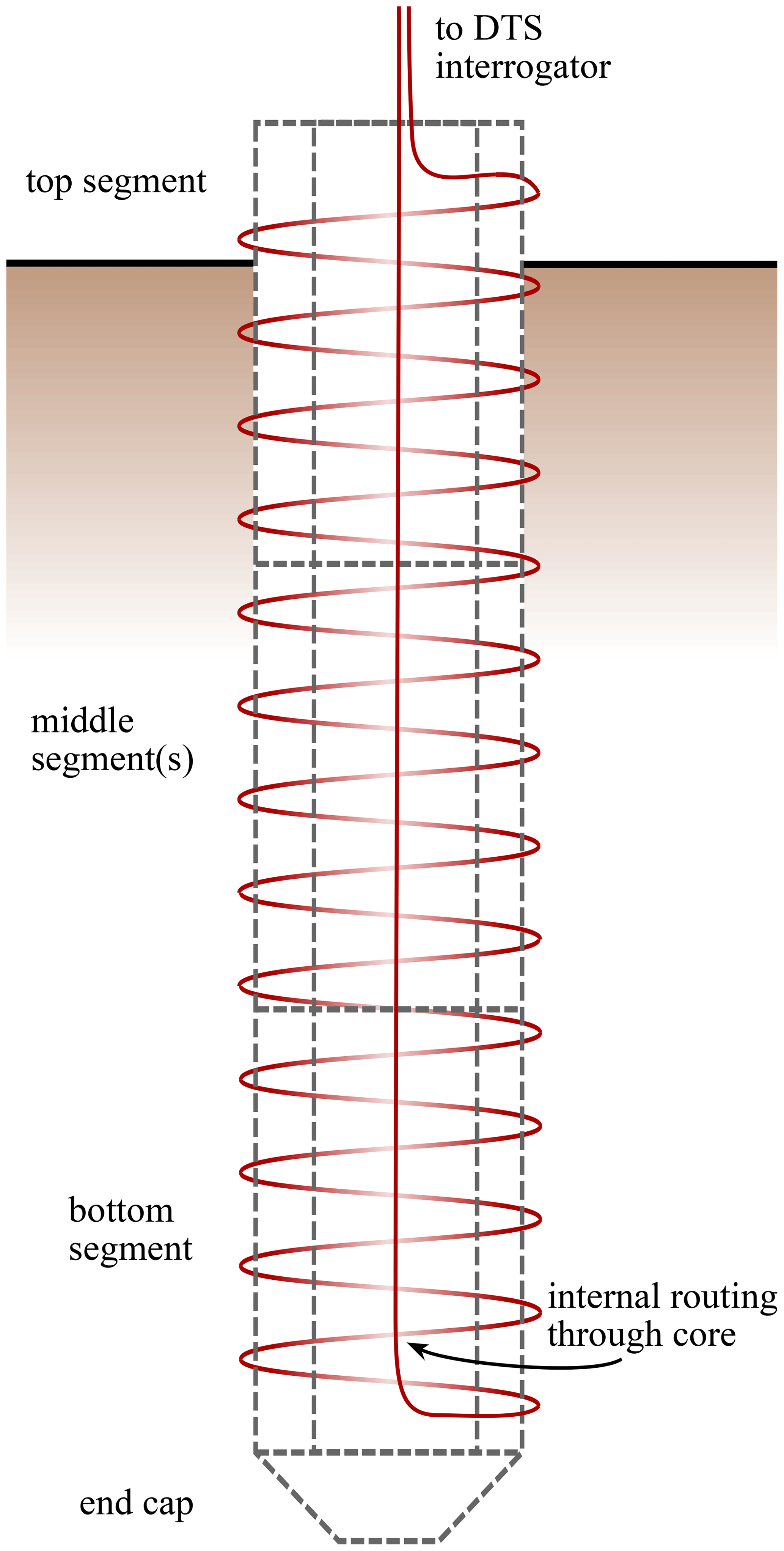
Figure 2Schematic drawing illustrating an installed probe, with a top section, single middle section, and bottom section. The fiber routing is illustrated in red.
To mitigate these problems, a protruding screw thread is incorporated into the design (Fig. 1). This creates a screw that makes good contact with the soil and provides a groove to install the fiber-optic cable into.
Inside the probe is an empty central tube. This space runs vertically through the probe and allows the routing of the fiber-optic cable back to the top of the probe. During assembly it is filled with expanding polyurethane foam to prevent heat transport and to seal out moisture. Hexagonal protrusions and slots are present at the top and bottom of the segments to make alignment easier during assembly. The diameter of the probe (75 mm, excluding the protrusions) was chosen to fit with our available augers to ensure compatibility between the dug hole and the probe.
For installation, a tool was designed. The tool engages into the holes at the top of the probe (Fig. 1) and has handles to allow the probe to be screwed into a pre-drilled hole. The tool can be seen in Fig. 3. After installation, the three holes are filled with printed plastic cylinders.
2.2 Fused-filament 3D printing
To manufacture this design we used consumer-grade 3D-printing technology. The most common consumer-grade 3D printers make use of the “fused-filament fabrication” method, where a computer-guided “extruder” heats up a plastic filament and deposits it into the right location to form an object (Chua et al., 2003). The extruder can only print lines that are the width of the nozzle (most commonly 0.4 mm). The printing is done layer by layer to slowly build up an object on the vertical axis. A limitation of this method of 3D printing is that new layers have to be supported by layers below, which puts a limitation on the shapes that can be printed without adding support material. So-called “overhangs” are possible but have a maximum angle of around 50° before the plastic will droop.
Table 1Thermal properties of commonly used 3D-printed plastics (PLA: polylactic acid; PETG: polyethylene terephthalate glycol) and a section of the printed probe, compared to typical values of sandy, silty, or clay soils. Note that the values for PLA and PETG are for objects made out of massive plastic, unlike most 3D-printed objects.
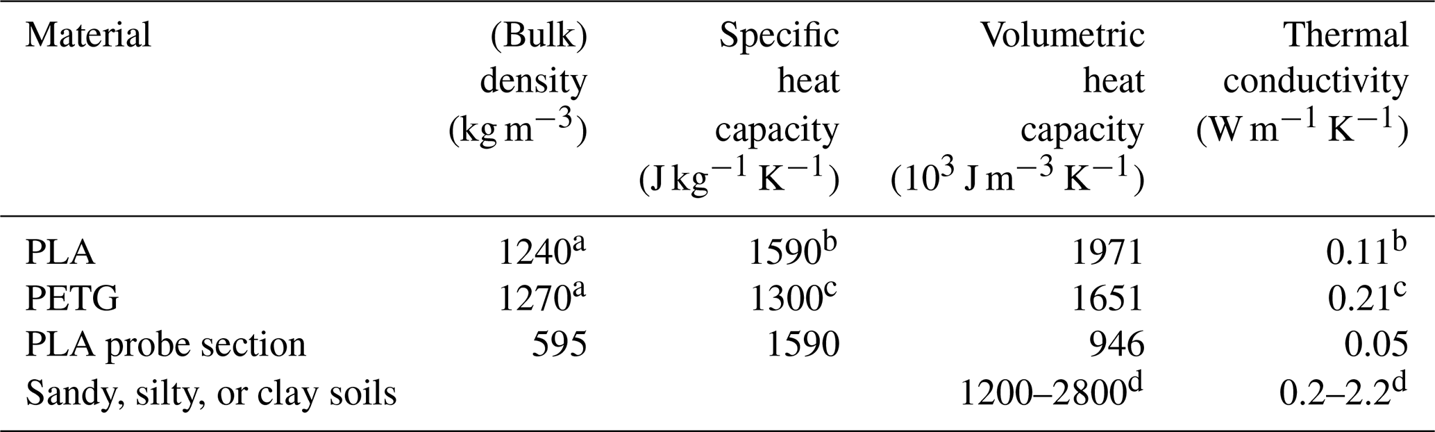
a Prusa Research (2018, 2020). b At ∼50 °C (Farah et al., 2016). c Rigid.ink (2017). d Over the full range of volumetric water content and air-filled porosity (Ochsner et al., 2001).
For our sensor, the plastics polylactic acid (PLA) and polyethylene terephthalate glycol (PETG) can be used as printing material. These two materials are easily printable on consumer-grade printers without the need for post-processing or special enclosures. PLA is not recommended for parts exposed to sunlight or in places where soil temperature exceeds 50 °C, as it is not heat-resistant or UV-stable. During our deployments of the probe we did not notice any degradation of the PLA or PETG plastic. While PLA is sometimes called “biodegradable”, it will barely degrade under many outdoor conditions (Bagheri et al., 2017). However, if the probe is to be placed in a more aggressive medium or needs to be relied on for a long time, ABS is a more resistant polymer.
The bulk density of printed objects can be substantially lower than the material density, as only the shell is made of solid plastic. In contrast, the internal volume is printed with so-called “infill”. This infill can take on different structures. Generally, the infill of a print is set to a certain percentage of the volume, e.g., an infill of 40 % means that 40 % of the internal volume consists of plastic and the remaining 60 % is air. The bulk density of a printed part can be determined by dividing the final weight of the printed part by the volume the part takes up (as derived from the 3D model). The chosen infill structure will depend on the required properties. In this case we chose a “cubic” infill, which will fill the volume with tessellated cubes. This structure will create enclosed pockets of air, which will hinder convection and, as such, reduce the heat flux through the printed part.
The material out of which the probe is constructed has quite a high heat capacity (Table 1). However, due to the hollow structure of the 3D-printed parts and the polyurethane foam core of the probe, the bulk thermal conductivity and heat capacity will be lower than the soil.
A middle section of the probe printed in PLA plastic has an effective infill of 48 %: more than half of the volume of the object consists of air pockets. This results in a heat capacity which is lower than that of most soils, even when the soil has a high fraction of air-filled pores. The effective thermal conductivity is at least a factor of 4 lower than that of dry soils, thus causing a minimal effect of the probe itself on the distribution of temperature in the soil.
2.3 Probe assembly
The parts are 3D-printed on a Prusa MK3 printer (Prusa Research, Prague, Czech Republic), using a Prusament PLA filament for all segments embedded in the soil and a Prusament PETG filament for the top (Prusa Research, 2018, 2020). No post-processing of the printed parts was needed. All segments are glued together using cyanoacrylate adhesive (“superglue”). We used five segments, making the total length of the probe 50 cm, out of which 45 cm has a groove for the fiber-optic cable. The remaining 5 cm is smooth.
A fiber-optic cable with a diameter of 1.6 mm is routed via the top through the hole at the bottom of the helix. The cable is then coiled around, using the groove as a guide. While the cable is coiled, it is glued in place using cyanoacrylate glue, which will provide a good bond between the cable and the PLA or PETG plastic. As such a small amount of glue is used, we neglect its thermal properties. When getting near the end of the spiral, the rest of the cable will have to be routed through the top hole. After this is done the remaining part of the spiral can be glued in place. When the spiral is in place, the bottom cap can be added to the probe, and the core can be filled with expanding polyurethane foam. This filling will prevent vertical transport of heat or water ingress through the core of the probe. Finally, the top cap can be installed to finish the probe.
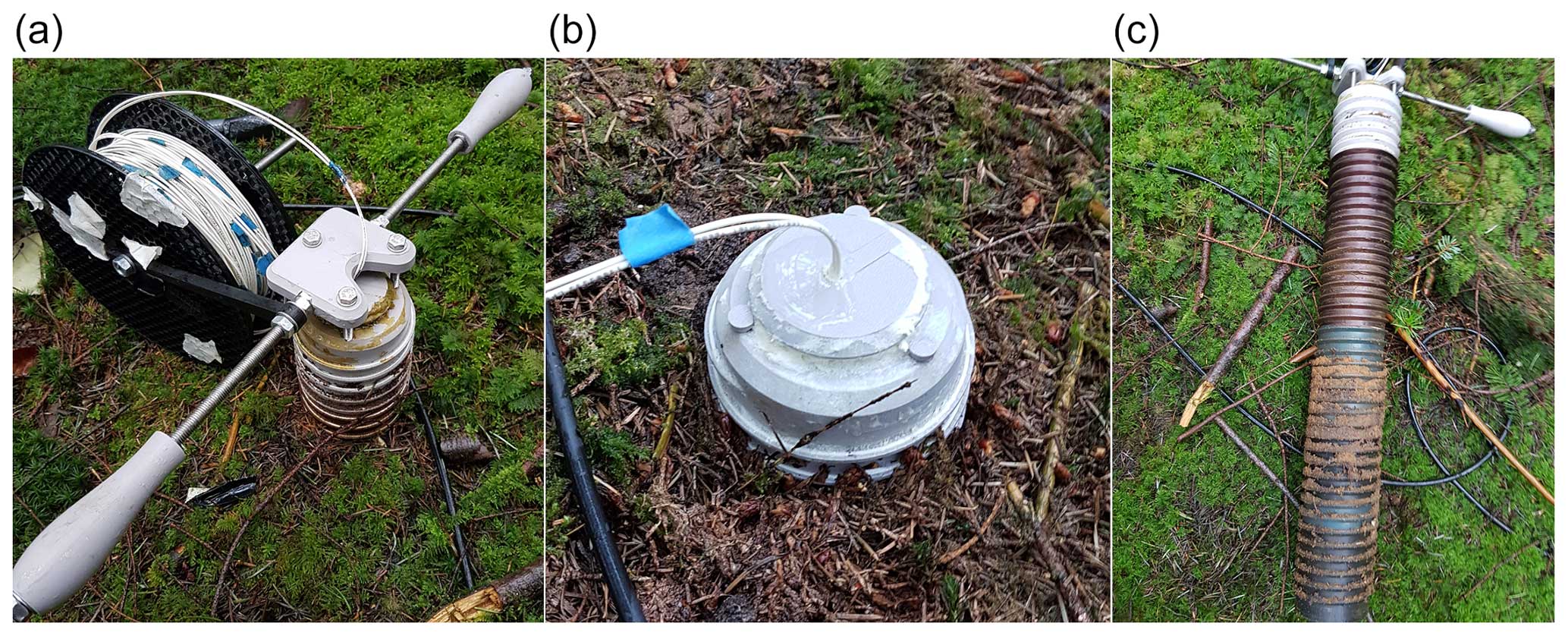
Figure 3Installing the DTS probe using the installation tool (a), the probe during installation (b), and the probe after removal (c).
2.4 Probe and reference sensor installation
The probe was tested at the Speulderbos site in the Netherlands (52°15′ N, 5°41′ E). The probe was installed near the flux tower at the site, which is located in a plot of ∼34 m tall Douglas fir trees (Pseudotsuga menziesii). The forest floor is mostly in the shade, except for short periods during sunny days where the light filters through the canopy. The soil on the forest floor has a 1–4 cm layer of moss and needles (O-horizon), followed by a dark A-horizon of around 4 cm in depth. This is followed a sandy C-horizon up to at least 40 cm. Due to the location being on a sandy hill, the groundwater is many meters deep (Tiktak and Bouten, 1994), and, as such, the soil is always unsaturated.
The soil probe was tested between 15 July and 30 September 2020. To install it, a layer of moss and needles was carefully removed and placed to the side. A hole was pre-drilled using an auger (75 mm diameter), and the probe was inserted into the soil by screwing it in place, leaving the top 3 cm sticking out (Fig. 3). After this, some of the sand that was removed with the auger was flushed back in using water, until no more sand flushed down. Some of the removed moss and needles were carefully placed back around the probe to restore the previous soil cover.
For reference, four Onset TMCx-HD temperature sensors were placed into the soil at a distance of ∼50 cm from the DTS probe. The sensors were connected to an Onset HOBO 4-Channel External Data Logger (HOBO U12-008). In this setup the temperature sensors had a manufacturer-specified accuracy of ±0.25 K. A hole was dug, and the sensors were horizontally inserted into the soil at depths of 0, 10, and 30 cm (Fig. 4). The litter layer consisting of moss, twigs, and needles had a depth varying between 2 and 5 cm. Another temperature sensor was inserted within the litter layer, approximately 2.5 cm above sensor at the soil–litter interface. The depth of this sensor will be represented by a value of −2.5 cm.
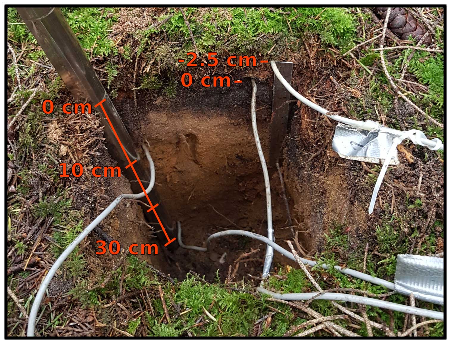
Figure 4Installation of reference sensors. One sensor was placed in the litter layer (2.5 cm above the soil–litter interface) and the others at depths of 0, 10, and 30 cm relative to the soil–litter interface. Note the decreasing organic content with depth.
2.5 Fiber-optic configuration and calibration
To perform the DTS measurements, an ULTIMA-M (Silixa Ltd., Elstree, UK) DTS unit was used. The ULTIMA-M was housed in a small container on the forest floor. The DTS probe consisted of one long FO cable without splices. From the DTS machine, the cable was routed out of the container, through a heated bath, and through a bath at ambient temperature. Both baths were kept mixed using aquarium air pumps with air stones. After the baths, the cable was lead to the measurement location under a suspended steel cable to avoid rodents and to protect the fiber from falling branches. After going through the 3D-printed probe, the FO cable was routed back under the steel cable, through both baths, and back into the container. Originally the setup was intended to be double-ended, where the fiber is interrogated from both sides so as to improve calibration. Due to rodent damage to the container, which occurred near the start of the measurement period, the fiber was only measured in a single-ended configuration. This could cause a small systematic error in areas where the fiber is strained, such as in the tight coil of the probe. To ensure the accuracy of the measurements, data from the first day (when the fiber was not damaged yet) were calibrated in both single- and double-ended configurations. The difference between the two was insignificant, and, as such, we proceeded with calibrating the DTS data in a single-ended configuration during the entire measurement period.
As the DTS measurements will only provide temperature as a function of the length along the optical fiber, these coordinates have to be transformed into depth values. This consists of two steps: translating the scale from meters along the fiber to centimeters along the coil by using the dimensions of the coil (radius, pitch, and height) and aligning the soil surface of the probe. The surface can be aligned (“benchmarked”) by doing a heat trace experiment, where a specific section of the coil (e.g., the part sticking out above the surface) is heated or cooled and the location along the length of the fiber where there is a sharp temperature spike is noted down. Alternatively, the probe can be aligned by comparing its temperature to the temperature of a reference temperature sensor at a known depth and by minimizing the difference between the two. In this study the final depth alignment of the probes was performed using the reference sensor at 10 cm. This depth was chosen because small local effects will average out across the soil. To avoid misalignment due to a constant bias between the two sensors, the amplitude of the diurnal temperature oscillation was used for alignment.
The dimensions of the coil and the DTS unit used for the study can also be used to determine the effective vertical resolution of a deployed probe. The ULTIMA-M unit has a sample rate of 25 cm and a spatial resolution of approximately 65 cm. It is common for DTS interrogators to sample at a higher resolution than what can be resolved for an individual data point. With the probe's 250 mm circumference, we have a vertical sampling resolution of 1.0 cm, corresponding to a spatial resolution of 2.6 cm. In cases where a device such as the Silixa ULTIMA-S is used to measure the same probe, the spatial resolution can be as small as 1.4 cm.
2.6 Determining soil diffusivity
The thermal diffusivity of a medium can be determined by inverse modeling (that is, by using a measured temperature profile through time). If we assume that the medium is homogeneous and that heat exchange is uniform at the surface (1D heat flow), the diffusion of heat through the soil can be described by the following equation:
where T is the soil temperature (K) at a certain depth z (m), t is the time (s), and D is the thermal diffusivity (m2 s−1). With only a temperature profile over time and depth, we cannot discern between the thermal conductivity, λ (W m−1 K−1), and the heat capacity, C (J m−3 K−1). This would require that soil properties be determined in a lab or that a heat flux plate be installed next to the measured profile. Note that in Eq. (1) the effects of latent heat flux or heat transported by the movement of air or water are neglected (Steele-Dunne et al., 2010).
Since the observations provide information on the soil temperature over depth and time, in principle the effective D could be calculated directly from the discretized version of Eq. (1). However, attention has to be given to the proper estimation of the second derivative because small observational errors may lead to a large uncertainty. Here we choose to estimate the diffusivity by fitting a numerical model of Eq. (1) to the measured temperature data, assuming that the diffusivity is constant in time over the period that is studied. We used a (second-order) central finite difference equation (Vuik et al., 2007) to describe the evolution of temperature through time for a section between two depths. The measured temperatures at the top and bottom of this section are prescribed, and the temperature in the middle is modeled with an estimate for the diffusivity. By comparing the modeled temperature to the measured temperature the difference can be minimized, and, as a result, the apparent diffusivity is determined.
Due to the large number of measurement points of the DTS probe, this equation can be used to determine the thermal diffusivity of the soil as a function of depth over the entire vertical profile. This could be expanded upon by incorporating more nearby measurement points for more accuracy, instead of the three points of Eq. (2).
While Eq. (2) has equidistant spacing, this is not necessarily required. For an irregularly spaced sampling, such as with the separate reference probes, the equations can be adjusted (Fornberg, 1988; Taylor, 2016). However, as the reference sensors only measured the depth at four locations, the thermal diffusivity can only be calculated for two (overlapping) sections.
3.1 Sample temperature profile
To demonstrate what the data from the probe look like, Fig. 5 shows the evolution of the soil temperature profile over a 24 h period: 1 August 12:00 LT until 2 August 12:00 LT.
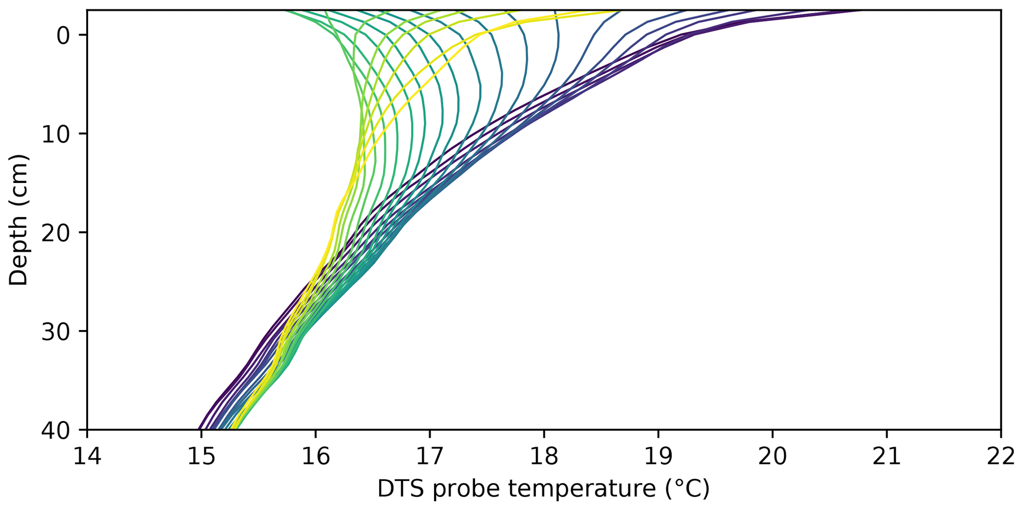
Figure 5Temperature over depth as measured by the DTS probe. Hourly data from noon on 1 August 2020 (dark purple) to noon on 2 August 2020 (yellow). The highest and lowest surface temperature occurred at 13:00 and 05:00 LT, respectively.
Starting at midday, the temperature profile is warmest at the top, cooling monotonously towards the deepest measurement at 40 cm depth. Soon after this point in time the soil near the surface starts cooling continuously until early morning. However, the soil below around 30 cm depth continues warming throughout the entire period shown (probably as a result of a long timescale, i.e., seasonal or trend in the weather). Note the extremely large gradients near the surface. Those gradients are very difficult to measure accurately using traditional temperature sensing. During the night the surface cools down the most, creating a zone 10–15 cm below the surface which is warmer than the soil both above and below. This local maximum persists until the soil warms up in the morning and a monotonous profile returns. Due to the very exact vertical spacing and high resolution of the DTS probe, phenomena such as this “hockey stick” profile can be observed.
The soil temperature deeper down was continuously the coldest, as both 1 and 2 August were relatively warm days. A downward heat flux at 40 cm was observed from the start of the measurement period (15 July) until late September.
3.2 Comparison with reference sensors
To compare the probe with the reference temperature sensors, the root-mean-square error (RMSE) between the DTS probe and the reference sensors is computed. However, to reduce any systematic biases between the probe and the reference sensors, the data are first detrended using a 5 d moving average. Systematic biases in the temperature can have their origin in, for example, a slight difference in calibration between the probe and the reference sensors. The mean biases between the four reference sensors and the DTS probe ranged between 0.10 and 0.30 K, within the expected uncertainty of the reference sensors and DTS measurements.
Figure 6 shows a good agreement between the DTS probe and the reference sensors, apart from the reference sensor at the soil–litter interface. Note that the largest error is also expected near the top where the diurnal amplitude is largest (no scaling of the error is applied). Even though the probe and the reference sensors were placed in relatively close proximity to each other, variations in the thickness of the litter layer could cause discrepancies near the surface. An additional source of uncertainty is the (horizontal) inhomogeneity of the soil properties and soil temperature. These will affect the DTS probe differently compared to traditional measurements. As the path of the fiber-optic cable is a helix, the measurement represents a spatial average along part of that helical path, instead of a single point in space. This will cause some (horizontal) spatial averaging. The measurement points near the surface could also be affected by the measurement resolution of the DTS unit, as the data point at −2.5 cm will still be slightly influenced by the temperature at around −3.8 cm.
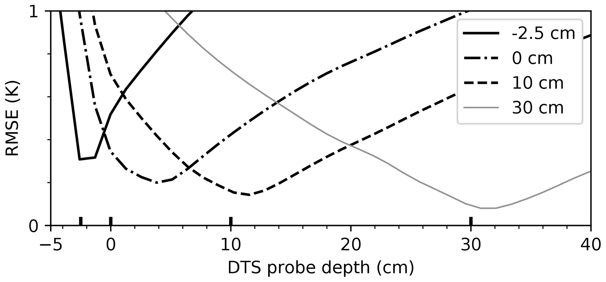
Figure 6Root-mean-square error (RMSE) of the DTS probe temperature compared to the reference sensors for the four available depths. The 0 cm depth is the soil–litter interface, and the −2.5 cm depth represents the temperature in the moss and litter layer.
A second way to compare the probe to the reference sensors is to study how much the diurnal variations in temperature are dampened as depth increases. By comparing the data in this fashion, biases in the absolute temperature are not relevant. Figure 7 shows the temperature variance as a function of depth (after detrending using a 5 d running mean, to only study the diurnal temperature variation). The variance decreases most strongly in the litter layer and flattens off deeper into the soil. The reference sensors agree mostly with the DTS probe. As the calibration was performed with a 10 cm probe, both agree by definition. However, the litter and the 30 cm sensors seem to be in agreement with the DTS probe as well. The sensor at the soil–litter interface deviates again, just as it did in the previous results. Again, it seems that the deviating reference sensor should be at ∼4 cm depth, just as Fig. 6 shows. However, the physical distance between the reference sensors in the litter and the deviating sensor is 2.5 cm, as can be seen from the ruler in Fig. 4. The source of the deviation is unlikely to be a too-low spatial resolution of the DTS data, as their spatial resolution is 3 cm.
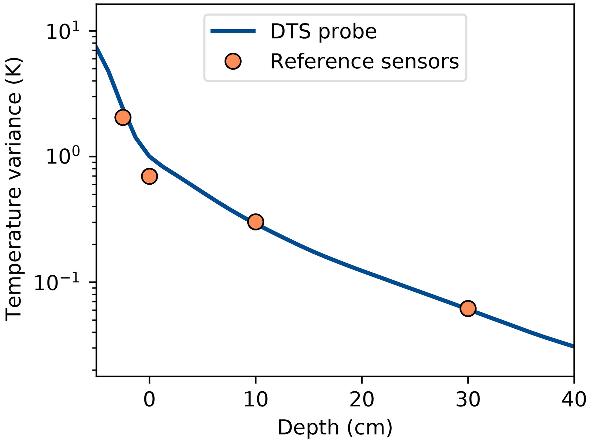
Figure 7Relationship between temperature variance and depth for the DTS probe and reference sensors. Depth values smaller than 0 cm denote parts of the coil possibly sticking out above the surface. Variance was determined for the whole dataset after detrending using a 5 d running mean.
Between depths of 15 to 40 cm, the DTS probe shows an approximately linear decrease in the logarithm of the temperature variance. This exponential dampening is expected when the soil thermal properties do not vary significantly over depth (Moene and van Dam, 2014). The stronger the slope is, the stronger the dampening. Just above the surface, which is covered by a layer of moss and litter, dampening is strongest. Deeper down, the dampening is weaker due to the lower organic matter content and higher soil density.
3.3 Thermal diffusivity
The availability of an almost continuous temperature profile by the DTS probe allows for the determination of soil thermal diffusivity as a function of depth. As there are many data points distributed over the depth, the thermal diffusivity can be estimated in many more intervals compared to with standard sensors, as at least three measurements of temperature are needed to compute the diffusivity. For the reference sensors only two diffusivity values could be computed, using either the sensors at −2.5, 0, and 10 cm or the sensors at 0, 10, and 30 cm. For the DTS probe data we chose to estimate the diffusivity over increasingly large intervals, from a 2.5 cm wide interval near the surface to a 10 cm wide interval near the deeper measurement points. By aggregating over larger intervals (in space or in time), the uncertainty in the DTS-measured temperature can be reduced. Here the aggregation was required as the signal becomes weaker the deeper one goes down into the soil, causing a lower signal-to-noise ratio and making the uncertainty in the estimate of diffusivity higher. A difficulty of the separate reference sensors is that any uncertainty or error at relative depths will directly translate into uncertainty or errors in the diffusivity estimate. If, for example, sensors are slightly further away in reality compared to how they are assumed to be, a higher diffusivity value will be found.
Figure 8 shows the computed diffusivity values as functions of both time and space. In time, the DTS probe and the reference sensors show a very similar pattern in the variations of diffusivity, with just a slight difference in the absolute value. As we see in Fig. 7 that the second reference sensor correlated better with the probe's temperature at 4 cm depth, the diffusivity values of the reference data with this adjusted sensor were calculated. These data show a pattern in the diffusivity over time that correlated less with the DTS probe data, although the mean error is smaller. The adjusted data show barely any variation in diffusivity over depth.
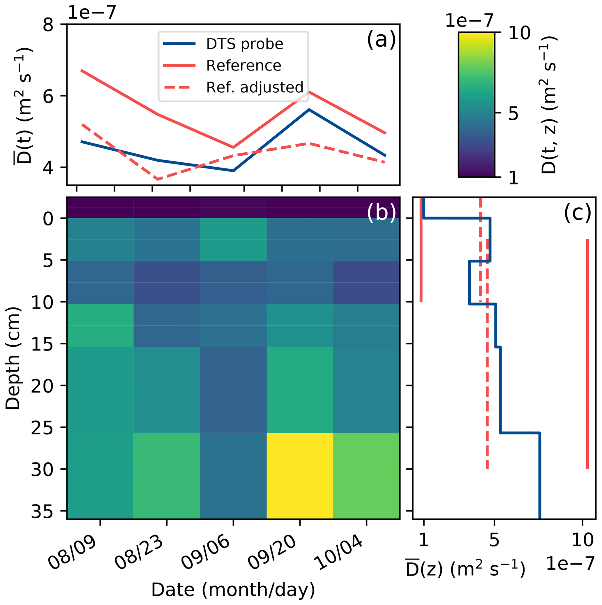
Figure 8(a) Mean diffusivity of the entire profile as a function of time, of both the reference sensors and the DTS probe. The dashed red line shows the reference if the second sensor depth is assumed to be at 4 cm instead of at 0 cm. (b) The diffusivity as measured by the DTS probe as a function of depth and time. (c) Mean diffusivity as a function of depth, of both the reference sensors and the DTS probe.
The change in diffusivity over time is to soil moisture; however, for sandy soils this is non-linear with very low moisture contents (under 0.07 kg kg−1; Abu-Hamdeh, 2003). With higher moisture contents, the thermal diffusivity of sandy soils is relatively insensitive to moisture and typically has values around m2 s−1 (Abu-Hamdeh, 2003; Moene and van Dam, 2014).
Over depth the data of the DTS probe show a lot more resolution, from the less-diffusive litter layer at the top (dark blue) to higher diffusivity values deeper down (green and yellow). These values of diffusivity vary due to variations in the soil composition and structure, depending on the content of organic matter or, e.g., gravel. Near the surface the reference sensors at the DTS probe agree in the diffusivity, but for the deeper layers the reference sensors estimate a higher value. The value derived using the DTS probe is closer to the expected value for sandy soils. The two methods previously agreed in the temperature variance at depths of 10 and 30 cm, and, as such, the deviating sensor at 0 cm would be the most likely cause of the error. Even a slight misalignment such as inserting the reference sensor at an angle could cause the actual measurement depth to deviate by 1 cm or more.
3.4 Outlook
While the DTS-based soil temperature probe does perform well and could provide more information than conventional sensors, it is important to consider the cost of DTS interrogators. With the high cost associated with these devices (over EUR 50 000) and the many other possible applications for them (Selker et al., 2006; De Jong et al., 2015; Hilgersom et al., 2016; des Tombe et al., 2018; Izett et al., 2019; Heusinkveld et al., 2020), it would not be logical to use them for soil temperature measurements alone. Even so, the probes can be integrated within a network of other DTS measurements of, for example, air temperature or horizontally distributed soil temperature. As long as the DTS interrogator has the available measurement length, the FO cables of the different setups can be spliced together into a single continuous fiber, and the entire setup can be measured at once.
To make calibration easier and less dependent on calibration baths, two standard soil temperature sensors could be integrated into the probe. This would allow calibration of the probe even if its more fragile FO cable is spliced to a more manageable and rugged FO cable. As a bonus the calibration baths would not be required anymore, which could simplify the setup.
Lastly, the coil does not need to be fully installed into the soil, and it can be allowed to stick out into the vegetation (if present). This way, some indication of the temperature profile inside the vegetation can be obtained, which can be used to determine the heat transfer through the vegetation (van der Linden et al., 2022). Note that, due to the much lower conductivity of air, the coil will have a slow response to temperature changes. Additionally, both incoming and outgoing solar radiation can pose issues and cause a bias in the measurement (see Schilperoort, 2022, Sect. 3).
In this study we presented a design for a DTS-based soil temperature probe, and we tested its performance in the field. The results were in general agreement with the reference sensors and were able to show more detail than standard sensors are capable of. It was possible to determine the thermal diffusivity of the soil at resolutions down to ∼8 cm; however, this can be improved to 4 cm with a more detailed DTS unit. With higher-resolution temperature data, the thermal properties of layers in the soil can be determined at a higher resolution.
Although this study only looked at the accuracy of the temperature measurement, the sensor can be expanded upon by using active heat tracer experiments. This would involve integrating an electrical conductor into the probe, e.g., a metal-tube fiber-optic cable, and heating it by using its electrical resistance (Bakker et al., 2015; van Ramshorst et al., 2020; Simon et al., 2021). If the power is supplied in a pulsed manner, the transient response can be studied to derive the heat capacity and thermal conductivity over depth (Sayde et al., 2010; Striegl and Loheide II, 2012; He et al., 2018). Using these properties, the soil moisture over depth can also be inferred, e.g., as in Wu et al. (2020). In this case two separate probes can be used, where one measures the undisturbed background soil temperature and the other measures the thermal properties of the soil. As soil moisture is an important variable in surface hydrology and land‐-atmosphere interactions, the continuous monitoring with a combination of vertical and horizontal distributed measurements could provide the best of both: capturing spatial heterogeneity while not sacrificing the accuracy.
The design files for all parts of the 3D-printed probe, including the installation tool, are available at https://doi.org/10.5281/zenodo.10984607 (Schilperoort, 2021), along with 3D renders of all parts. The processed measurement data are openly available on Zenodo: see Schilperoort and Jiménez-Rodríguez (2023) (https://doi.org/10.5281/zenodo.8108401).
BS designed and fabricated the probe. BS and CJR carried out the field measurements. BS processed the data and performed the data analysis. BS prepared the article with contributions from all co-authors.
The contact author has declared that none of the authors has any competing interests.
Publisher's note: Copernicus Publications remains neutral with regard to jurisdictional claims made in the text, published maps, institutional affiliations, or any other geographical representation in this paper. While Copernicus Publications makes every effort to include appropriate place names, the final responsibility lies with the authors.
This paper was edited by Lev Eppelbaum and reviewed by Bartosz Zawilski and one anonymous referee.
Abu-Hamdeh, N. H.: Thermal Properties of Soils as affected by Density and Water Content, Biosyst. Eng., 86, 97–102, https://doi.org/10.1016/S1537-5110(03)00112-0, 2003. a, b
Bagheri, A. R., Laforsch, C., Greiner, A., and Agarwal, S.: Fate of So‐Called Biodegradable Polymers in Seawater and Freshwater, Global Challeng., 1, 1700048, https://doi.org/10.1002/gch2.201700048, 2017. a
Bakker, M., Caljé, R., Schaars, F., van der Made, K., and de Haas, S.: An active heat tracer experiment to determine groundwater velocities using fiber optic cables installed with direct push equipment, Water Resour. Res., 51, 2760–2772, https://doi.org/10.1002/2014WR016632, 2015. a
Bense, V. F., Read, T., and Verhoef, A.: Using distributed temperature sensing to monitor field scale dynamics of ground surface temperature and related substrate heat flux, Agr. Forest Meteorol., 220, 207–215, https://doi.org/10.1016/j.agrformet.2016.01.138, 2016. a
Briggs, M. A., Lautz, L. K., McKenzie, J. M., Gordon, R. P., and Hare, D. K.: Using high‐resolution distributed temperature sensing to quantify spatial and temporal variability in vertical hyporheic flux, Water Resour. Res., 48, W02527, https://doi.org/10.1029/2011WR011227, 2012. a
Chua, C. K., Leong, K. F., and Lim, C. S.: Rapid Prototyping: Principles and Applications, World Scientific, Singapore, ISBN 9789812381170, 2003. a
De Jong, S. A. P., Slingerland, J. D., and Van De Giesen, N. C.: Fiber optic distributed temperature sensing for the determination of air temperature, Atmos. Meas. Tech., 8, 335–339, https://doi.org/10.5194/amt-8-335-2015, 2015. a
des Tombe, B. F., Bakker, M., Schaars, F., and van der Made, K. J.: Estimating Travel Time in Bank Filtration Systems from a Numerical Model Based on DTS Measurements, Groundwater, 56, 288–299, https://doi.org/10.1111/gwat.12581, 2018. a
Dong, J., Steele‐Dunne, S. C., Ochsner, T. E., Hatch, C. E., Sayde, C., Selker, J., Tyler, S., Cosh, M. H., and van de Giesen, N.: Mapping high‐resolution soil moisture and properties using distributed temperature sensing data and an adaptive particle batch smoother, Water Resour. Res., 52, 7690–7710, https://doi.org/10.1002/2016WR019031, 2016. a, b
Eppelbaum, L., Kutasov, I., and Pilchin, A.: Applied Geothermics, in: Lecture Notes in Earth System Sciences, Springer, Berlin, Heidelberg, ISBN 978-3-642-34022-2, https://doi.org/10.1007/978-3-642-34023-9, 2014. a
Farah, S., Anderson, D. G., and Langer, R.: Physical and mechanical properties of PLA, and their functions in widespread applications – A comprehensive review, Adv. Drug Deliv. Rev., 107, 367–392, https://doi.org/10.1016/j.addr.2016.06.012, 2016. a
Fornberg, B.: Generation of finite difference formulas on arbitrarily spaced grids, Math. Comput., 51, 699–699, https://doi.org/10.1090/S0025-5718-1988-0935077-0, 1988. a
He, H., Dyck, M. F., Horton, R., Li, M., Jin, H., and Si, B.: Distributed Temperature Sensing for Soil Physical Measurements and Its Similarity to Heat Pulse Method, Adv. Agron., 148, 173–230, https://doi.org/10.1016/bs.agron.2017.11.003, 2018. a
Heusinkveld, B. G., Jacobs, A. F., Holtslag, A. A., and Berkowicz, S. M.: Surface energy balance closure in an arid region: Role of soil heat flux, Agr. Forest Meteorol., 122, 21–37, https://doi.org/10.1016/j.agrformet.2003.09.005, 2004. a, b
Heusinkveld, V. W., Antoon van Hooft, J., Schilperoort, B., Baas, P., ten Veldhuis, M.-c., and van de Wiel, B. J.: Towards a physics-based understanding of fruit frost protection using wind machines, Agr.Forest Meteorol., 282–283, 107868, https://doi.org/10.1016/j.agrformet.2019.107868, 2020. a
Hilgersom, K., van Emmerik, T., Solcerova, A., Berghuijs, W., Selker, J., and van de Giesen, N.: Practical considerations for enhanced-resolution coil-wrapped distributed temperature sensing, Geosci. Instrum. Method. Data Syst., 5, 151–162, https://doi.org/10.5194/gi-5-151-2016, 2016. a, b
Holtslag, A. A. M. and De Bruin, H. A. R.: Applied Modeling of the Nighttime Surface Energy Balance over Land, J. Appl. Meteorol., 27, 689–704, https://doi.org/10.1175/1520-0450(1988)027<0689:AMOTNS>2.0.CO;2, 1988. a
Izett, J. G., Schilperoort, B., Coenders-Gerrits, M., Baas, P., Bosveld, F. C., and van de Wiel, B. J. H.: Missed Fog?, Bound.-Lay. Meteorol., 173, 289–309, https://doi.org/10.1007/s10546-019-00462-3, 2019. a
Jansen, J., Stive, P. M., van de Giesen, N., Tyler, S., Steele-Dunne, S. C., and Williamson, L.: Estimating soil heat flux using Distributed Temperature Sensing, GRACE, Remote Sensing and Ground-based Methods in Multi-Scale Hydrology, 140–144, ISBN 978-1-907161-18-6, https://iahs.info/uploads/dms/16743.28-140-144-343-10-Jansen.pdf (last access: 15 April 2024), 2011. a
Moene, A. F. and van Dam, J. C.: Transport in the Atmosphere-Vegetation-Soil Continuum, Cambridge University Press, ISBN 9780521195683, https://doi.org/10.1017/CBO9781139043137, 2014. a, b
Ochsner, T. E., Horton, R., and Ren, T.: A New Perspective on Soil Thermal Properties, Soil Sci. Soc. Am. J., 65, 1641–1647, https://doi.org/10.2136/sssaj2001.1641, 2001. a
Prusa Research: Prusament PLA by Prusa Polymers, Tech. rep., Prusa Research, Prague, https://prusament.com/wp-content/uploads/2022/10/PLA_Prusament_TDS_2021_10_EN.pdf (last access: 18 April 2024), 2018. a, b
Prusa Research: Prusament PETG by Prusa Polymers, Tech. rep., Prusa Research a.s., Prague, Czech Republic, https://prusament.com/wp-content/uploads/2023/07/PETG_V0_ENG.pdf (last access: 18 April 2024), 2020. a, b
Rigid.ink: PETG data shet, Tech. rep., rigid.ink, Wetherby, UK, http://devel.lulzbot.com/filament/Rigid_Ink/PETG DATA SHEET.pdf (last access: 15 April 2024), 2017. a
Saito, K., Iwahana, G., Ikawa, H., Nagano, H., and Busey, R. C.: Links between annual surface temperature variation and land cover heterogeneity for a boreal forest as characterized by continuous, fibre-optic DTS monitoring, Geosci. Instrum. Method. Data Syst., 7, 223–234, https://doi.org/10.5194/gi-7-223-2018, 2018. a, b
Sayde, C., Gregory, C., Gil-Rodriguez, M., Tufillaro, N., Tyler, S., van de Giesen, N., English, M., Cuenca, R., and Selker, J. S.: Feasibility of soil moisture monitoring with heated fiber optics, Water Resour. Res., 46, W06201, https://doi.org/10.1029/2009WR007846, 2010. a, b
Schilperoort, B.: DTS-based 3D printing design for a soil temperature profiler, Zenodo [data set], https://doi.org/10.5281/zenodo.10984607, 2021. a
Schilperoort, B.: Heat Exchange in a Conifer Canopy: A Deep Look using Fiber Optic Sensors, Doctoral dissertation, Delft University of Technology, Delft, https://doi.org/10.4233/uuid:6d18abba-a418-4870-ab19-c195364b654b, 2022. a
Schilperoort, B. and Jiménez-Rodríguez, C. D.: Soil temperature profiles, measured using a coil-shaped fiber-optic distributed temperature sensor, Zenodo [data set], https://doi.org/10.5281/zenodo.8108401, 2023. a
Schilperoort, B., Coenders-Gerrits, M., Jiménez Rodríguez, C., van der Tol, C., van de Wiel, B., and Savenije, H.: Decoupling of a Douglas fir canopy: a look into the subcanopy with continuous vertical temperature profiles, Biogeosciences, 17, 6423–6439, https://doi.org/10.5194/bg-17-6423-2020, 2020. a
Selker, J. S., Thévenaz, L., Huwald, H., Mallet, A., Luxemburg, W., Van De Giesen, N., Stejskal, M., Zeman, J., Westhoff, M., and Parlange, M. B.: Distributed fiber-optic temperature sensing for hydrologic systems, Water Resour. Res., 42, 1–8, https://doi.org/10.1029/2006WR005326, 2006. a
Shehata, M., Heitman, J., Ishak, J., and Sayde, C.: High‐Resolution Measurement of Soil Thermal Properties and Moisture Content Using a Novel Heated Fiber Optics Approach, Water Resour. Res., 56, e2019WR025204, https://doi.org/10.1029/2019WR025204, 2020. a
Simon, N., Bour, O., Lavenant, N., Porel, G., Nauleau, B., Pouladi, B., Longuevergne, L., and Crave, A.: Numerical and Experimental Validation of the Applicability of Active‐DTS Experiments to Estimate Thermal Conductivity and Groundwater Flux in Porous Media, Water Resour. Res., 57, e2020WR028078, https://doi.org/10.1029/2020WR028078, 2021. a
Steele-Dunne, S. C., Rutten, M. M., Krzeminska, D. M., Hausner, M., Tyler, S. W., Selker, J., Bogaard, T. A., and Van De Giesen, N. C.: Feasibility of soil moisture estimation using passive distributed temperature sensing, Water Resour. Res., 46, 1–12, https://doi.org/10.1029/2009WR008272, 2010. a, b, c
Striegl, A. M. and Loheide II, S. P.: Heated Distributed Temperature Sensing for Field Scale Soil Moisture Monitoring, Ground Water, 50, 340–347, https://doi.org/10.1111/j.1745-6584.2012.00928.x, 2012. a
Taylor, C.: Finite Difference Coefficients Calculator, https://web.media.mit.edu/~crtaylor/calculator.html (last access: 15 April 2024), 2016. a
Tiktak, A. and Bouten, W.: Soil water dynamics and long-term water balances of a Douglas fir stand in the Netherlands, J. Hydrol., 156, 265–283, https://doi.org/10.1016/0022-1694(94)90081-7, 1994. a
van der Linden, S. J. A., Kruis, M. T., Hartogensis, O. K., Moene, A. F., Bosveld, F. C., and van de Wiel, B. J. H.: Heat Transfer Through Grass: A Diffusive Approach, Bound.-Lay. Meteorol., 184, 251–276, https://doi.org/10.1007/s10546-022-00708-7, 2022. a, b
van der Tol, C.: Validation of remote sensing of bare soil ground heat flux, Remote Sens. Environ., 121, 275–286, https://doi.org/10.1016/j.rse.2012.02.009, 2012. a
Van de Wiel, B. J. H., Moene, A. F., Hartogensis, O. K., De Bruin, H. A. R., and Holtslag, A. A. M.: Intermittent Turbulence in the Stable Boundary Layer over Land. Part III: A Classification for Observations during CASES-99, J. Atmos. Sci., 60, 2509–2522, https://doi.org/10.1175/1520-0469(2003)060<2509:ITITSB>2.0.CO;2, 2003. a, b
van Ramshorst, J. G. V., Coenders-Gerrits, M., Schilperoort, B., van de Wiel, B. J. H., Izett, J. G., Selker, J. S., Higgins, C. W., Savenije, H. H. G., and van de Giesen, N. C.: Revisiting wind speed measurements using actively heated fiber optics: a wind tunnel study, Atmos. Meas. Tech., 13, 5423–5439, https://doi.org/10.5194/amt-13-5423-2020, 2020. a
van Wijk, W. and de Vries, D.: Periodic temperature variations in a homogeneous soil, in: Physics of plant environment, North-Holland Publ. Co., Amsterdam, 102–143, https://doi.org/10.1002/qj.49709038628, 1963. a
Verhoef, A.: Remote estimation of thermal inertia and soil heat flux for bare soil, Agr. Forest Meteorol., 123, 221–236, https://doi.org/10.1016/j.agrformet.2003.11.005, 2004. a
Vogt, T., Schneider, P., Hahn-Woernle, L., and Cirpka, O. A.: Estimation of seepage rates in a losing stream by means of fiber-optic high-resolution vertical temperature profiling, J. Hydrol., 380, 154–164, https://doi.org/10.1016/j.jhydrol.2009.10.033, 2010. a
Vuik, C., van Beek, P., Vermolen, F., and van Kan, J.: Numerical methods for ordinary differential equations, VSSD, Delft, ISBN 9781281744555, 2007. a
Wu, R., Martin, V., McKenzie, J., Broda, S., Bussière, B., Aubertin, M., and Kurylyk, B. L.: Laboratory-scale assessment of a capillary barrier using fibre optic distributed temperature sensing (FO-DTS), Can. Geotech. J., 57, 115–126, https://doi.org/10.1139/cgj-2018-0283, 2020. a, b
Wu, R., Lamontagne-Hallé, P., and McKenzie, J. M.: Uncertainties in Measuring Soil Moisture Content with Actively Heated Fiber-Optic Distributed Temperature Sensing, Sensors, 21, 3723, https://doi.org/10.3390/s21113723, 2021. a
Xie, X., Lu, Y., Ren, T., and Horton, R.: Soil temperature estimation with the harmonic method is affected by thermal diffusivity parameterization, Geoderma, 353, 97–103, https://doi.org/10.1016/j.geoderma.2019.06.029, 2019. a