Research on the correction method of hydraulic fracturing in-situ stress testing based on MLP-KFold

Hydraulic fracturing serves as a critical in-situ stress testing technique, where the accurate determination of rock fracture pressure and closure pressure in fracturing intervals is essential for precise in-situ stress estimation. During hydraulic fracturing stress measurement, parameters including injection rate, viscosity, density, and compressibility ratio of fracturing fluid significantly affect the measurement accuracy of fracture and closure pressures, potentially introducing substantial errors in in-situ stress calculations. This study develops an MLP-KFold-based correction model for in-situ stress measurements by establishing a hydraulic fracturing dataset, incorporating fracturing fluid density, viscosity, injection rate, and corresponding rock fracture/closure pressures. Evaluation results demonstrate that the MLP-KFold model achieves superior performance with a coefficient of determination (R² = 0.9937) on test sets, outperforming Random Forest (Δ+1.89 %), Support Vector Regression (Δ+4.05 %), and BiLSTM (Δ+5.34 %). Key error metrics including MAE (0.518), MSE (0.646), and maximum error (1.945 MPa) remain at minimal levels. Field applications demonstrate significant reduction in average percentage differences of calculated stresses under different fracturing fluids (σ_H: −21.48 %, σ_h: −29.03 %), confirming its superior compensation effects. This research establishes a compensation model for hydraulic fracturing pressures based on a small-scale dataset, providing an effective technical approach for correcting field measurement data and compensating in-situ stress calculation results, thereby contributing to the accurate assessment of regional stress profile states.

1 Introduction

The stress that is stored within the undisturbed rock mass is referred to as geo-stress or in-situ stress, which is caused by factors such as the self-weight of the rock and geological tectonic movements (Mcgarr and Gay, 1978; Amadei and Stephansson, 1997). Regional in-situ stress measurement and estimation have important applications in earthquake prediction research, underground engineering construction, mining, and oil and gas extraction. With the increasing demand for energy and mineral resources and the continuous intensification of mining efforts in China, shallow mineral resources are gradually diminishing, and domestic mines are successively entering the stage of deep resource development. The “three highs” issues encountered in deep mining (high in-situ stress, high temperature, and high water pressure) (Xie, 2019) will become the focus and difficulty in the study of deep mining rock mechanics (He et al., 2005). Therefore, accurately determining the in-situ stress state of the deep development area is a necessary approach to solving the above problems.

Table 1 In-situ stress testing methods (Wang, 2014).

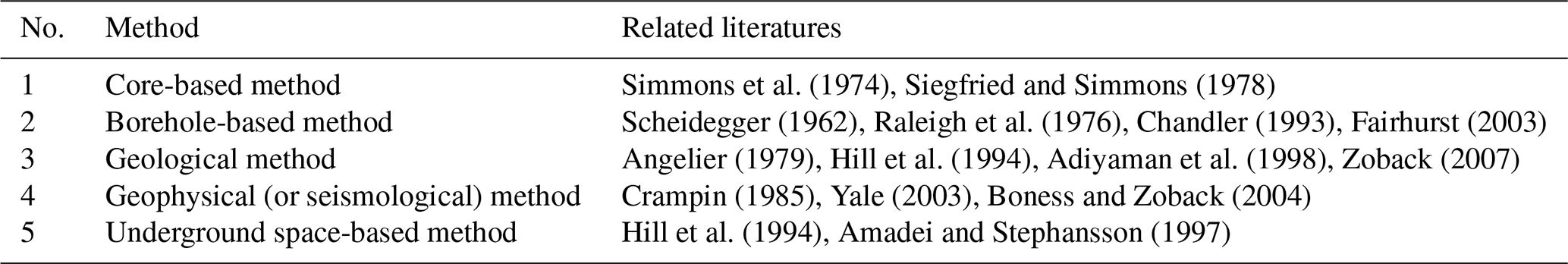
Observation and estimation of the in-situ stress state in the deep crust remain a major challenge in in-situ stress measurement. Scientists have proposed dozens of in-situ stress testing methods, which can be classified into five categories based on data sources, as described in Table 1.

The hydraulic fracturing method, a subset of borehole-based techniques, is currently the only known approach capable of directly measuring in-situ stress. Although theoretically unrestricted by depth, practical limitations – such as borehole conditions, testing technology, and temperature/pressure resistance of equipment – have resulted in very few successful hydraulic fracturing stress measurements worldwide at depths exceeding 1000 m (Zhang and Stephansson, 2010; Chen et al., 2019). Consequently, precise measurement and estimation of in-situ stress using hydraulic fracturing remains a critical research challenge both domestically and internationally.

The hydraulic fracturing method features a relatively simple and rapid testing process, along with straightforward data processing and analysis. However, during testing, deformation of drill pipes and packers, as well as external factors related to the fluid mechanics parameters of fracturing fluids (e.g., viscosity, density, compressibility, and injection rate), can significantly affect the measurements of rock breakdown pressure, closure pressure, and reopening pressure in the fracturing interval. Consequently, these influences also introduce errors in subsequent calculations of the maximum and minimum horizontal principal stresses, ultimately impairing the accurate estimation of in-situ stress. Related scholars have conducted in-depth research on the influence of fracturing fluid parameters such as flow rate, viscosity, and density on rock breakdown pressure and closure pressure. Ito and Hayashi (1991) and Chang et al. (2013) proposed that the tensile strength of rock increases with the injection rate. Zhou et al. (2013) and Zhang (2018) conducted laboratory hydraulic fracturing experiments, demonstrating that mud media with different densities significantly affect the measured values of rock breakdown. Matsunaga et al. (1993) and Ishida et al. (1997) confirmed in their studies on petroleum drilling that the viscosity of fracturing fluid influences rock breakdown. Wang et al. (2012) and Zhou et al. (2013) both used water as the fracturing fluid to analyze the effect of fluid compressibility on system compliance, which leads to errors in in-situ stress measurement. Tomac and Gutierrez (2017) employed a Bonded Particle Model (BPM) within the Discrete Element Method (DEM) framework to conduct coupled thermo-hydro-mechanical analysis, revealing that temperature gradients and fluid-rock compressibility ratios critically govern fracture dynamics in enhanced geothermal systems: the coupled convective-conductive thermal effects shorten primary fractures and induce secondary microcracks, while cold fluid infiltration reduces near-wellbore pressure accumulation to delay propagation, with compressibility ratio governing fracture velocity and dynamic viscosity modulating thermal damage extent. Liu et al. (2019) optimized hydraulic fracturing simulation experiments using the uniform design method and preliminarily analyzed the influence of different fracturing fluid media on breakdown pressure through regression fitting. Ma et al. (2024) utilized an LSTM to directly predict the breakdown pressure of horizontal wells in petroleum engineering, effectively establishing a nonlinear relationship between logging parameters and breakdown pressure in horizontal wells. Zou et al. (2025) investigated the influences of key parameters, including rock temperature, in situ stress, injection rate, fluid viscosity, azimuth of the radial borehole, and the number of radial boreholes on the fracture morphology and breakdown pressure, the breakdown pressure of radial borehole fracturing can be reduced by 14.1 %–43.7 % compared to conventional fracturing, which has been demonstrated that the increases in the vertical density of radial boreholes, injection rate, and fluid viscosity enhance the guiding ability of radial boreholes. Liu et al. (2024) proposed a horizontal-hole hydraulic fracturing based in-situ stress model incorporating fluid flow rate by conducting hydraulic fracturing fluid-solid coupling simulation tests to explore the effect of different fracturing fluid flow rates on fracture propagation and breakdown pressure in granite, and the model calculations matched test values with a relative error under 9 %, establishing a more precise in-situ stress calculation model for tunnel surrounding rock.

Measurement errors in rock breakdown pressure and closure pressure can lead to significant variations in the calculated maximum and minimum horizontal principal stresses, severely impacting the accuracy of hydraulic fracturing-based in-situ stress estimation (Wang et al., 2017). Accurately determining rock breakdown pressure and closure pressure has long been a challenging task. Reducing the errors in in-situ stress calculations caused by influencing factors such as fracturing fluid flow rate, viscosity, density, and compressibility – and establishing corresponding error compensation models – necessitates the application of machine learning and deep learning methods. This paper constructed a dataset based on laboratory hydraulic fracturing simulation experiments. For relatively small-scale datasets, we employed a multi-layer perceptron (MLP) with K-fold cross-validation (KFold) to develop correction models for breakdown pressure and closure pressure. This approach demonstrates high data utilization efficiency and stable performance evaluation, exhibiting certain advantages over other machine learning models. The proposed method holds significant theoretical and practical value for precise regional stress profile estimation, crustal stability assessment, earthquake prediction, and mine strata stability evaluation.

2 Principle of hydraulic fracturing in-situ stress testing

The classical hydraulic fracturing theory, based on the plane strain theory of elasticity, was proposed and refined by Haimson (1968). This theory is based on three key assumptions: First, rocks are considered to be homogeneous, linearly elastic, and isotropic materials, which means that the mechanical properties of rocks are the same in all directions, and there is a linear relationship between stress and strain; second, rocks are assumed to be porous media, and the fluid flow within the pores follows Darcy's Law, which states that the fluid flow rate is directly proportional to the pressure gradient; finally, it is assumed that one of the principal axes of the in-situ stress is parallel to the borehole axis. Based on these assumptions, the fractures induced by hydraulic fracturing are vertical and perpendicular to the direction of the minimum horizontal principal stress, as shown in Fig. 1.

Figure 1 Mechanical model and pressure curve diagram of hydraulic fracturing measurement.

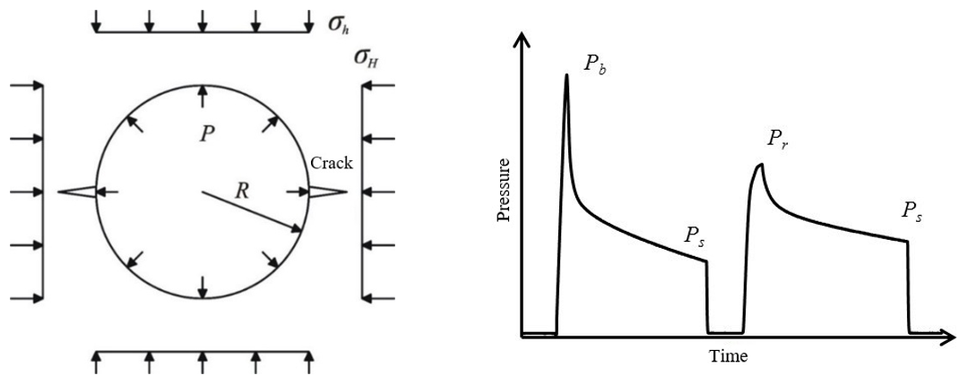
Using the stress field model and fracture criteria depicted in Fig. 1, the fracture values of the fractured rock section are shown below, according to the elastic theory (Timoshenko and Goodier, 1970):

$$\begin{array}{}\text{(1)}& {\displaystyle }{P}_{\mathrm{b}}=\mathrm{3}{\mathit{\sigma }}_{\mathrm{h}}-{\mathit{\sigma }}_{\mathrm{H}}+T\text{(2)}& {\displaystyle }{P}_{\mathrm{s}}={\mathit{\sigma }}_{\mathrm{h}}\end{array}$$

Here, σ_H and σ_h represent the maximum and minimum horizontal principal stresses, respectively, P_b and P_s represent the fracture pressure and closure pressure, respectively, and T represents the tensile strength of the rock. Equations (1) and (2) indicate that the fracture values of the rock are independent of the size of the borehole and the rock's elastic modulus, and are mainly determined by the tensile strength of the rock and the magnitude of the in-situ stress around the borehole. Therefore, accurately obtaining the fracture pressure, closure pressure, and tensile strength of the rock is key to improving the accuracy of hydraulic fracturing stress measurements.

3 Hydraulic fracturing dataset

3.1 Dataset construction

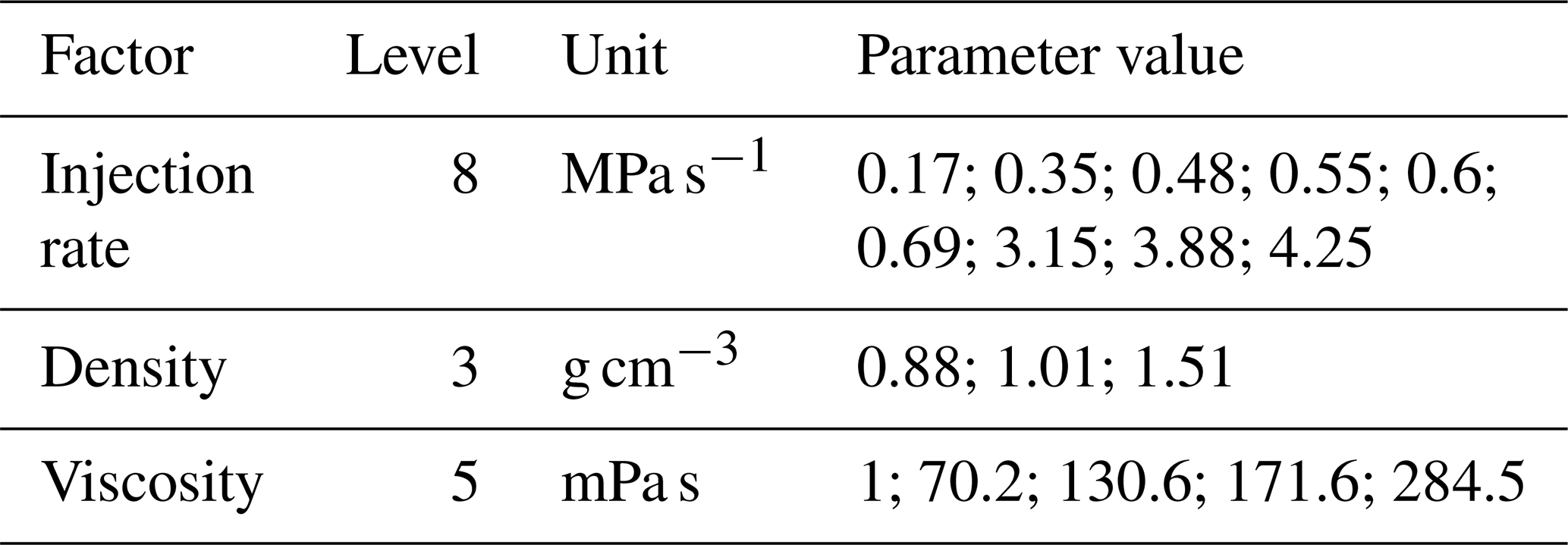
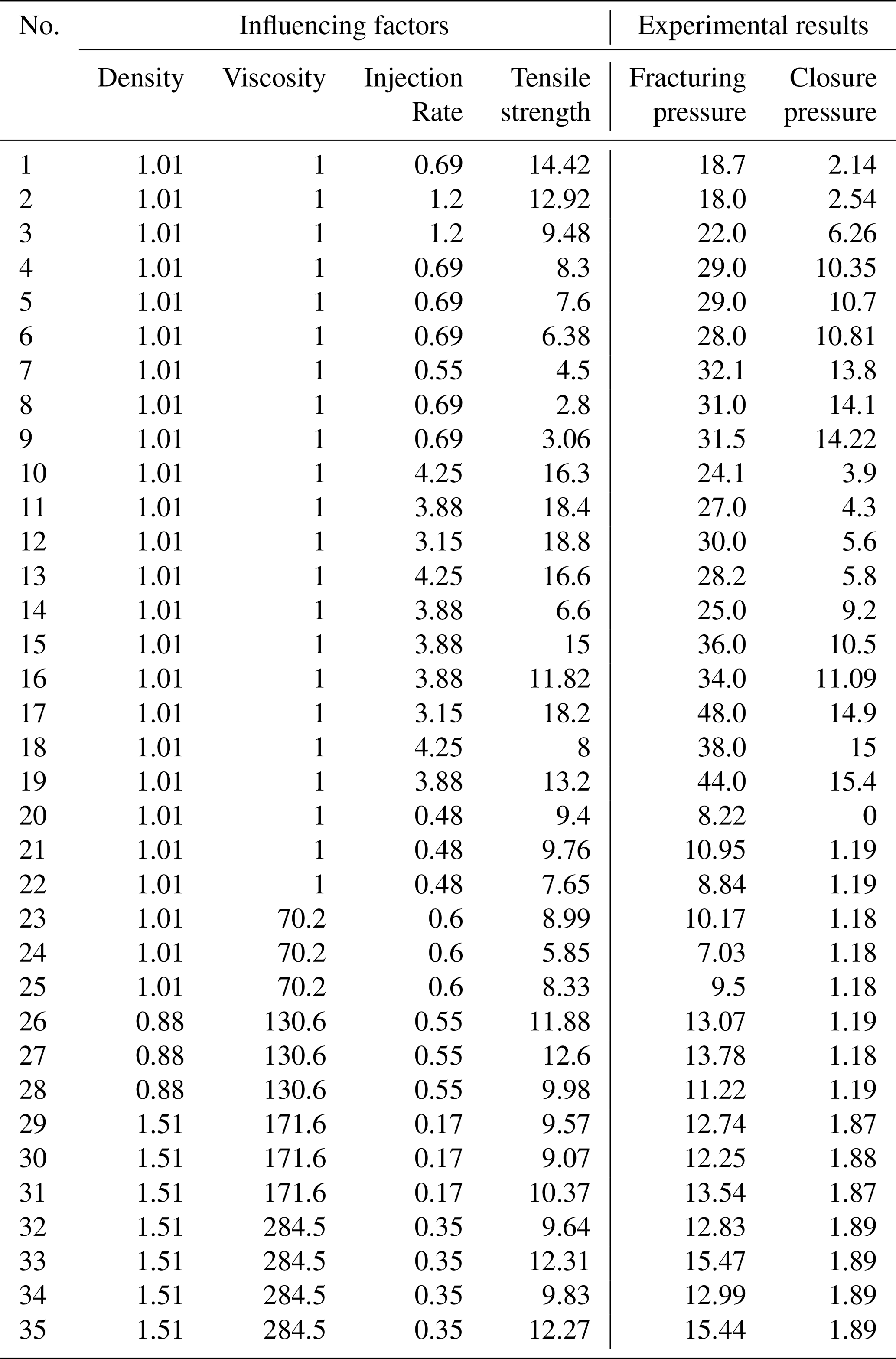
The fracturing fluids commonly used in hydraulic fracturing mainly include water-based, oil-based, foam-based and slurry-based types (Cuisiat and Haimson, 1992; Birdsell et al., 2015). In order to construct a dataset for hydraulic fracturing simulation experiments, this paper used a hollow cylinder test method to obtain fracture pressure and closure pressure data of granite using water-based, oil-based, and mud as fracturing fluid media. (Ito and Hayashi, 1991; Zhang, 2018). Table 4 summarizes various experimental factors and their corresponding levels.

The constructed hydraulic fracturing dataset was used for 35 cubic specimens with different tensile strengths, and 35 hydraulic fracturing simulation experiments were conducted based on 8-level injection rate, 2-level density, and 5-level viscosity (as shown in Table 2). The experimental results (fracturing pressure and closure pressure) are shown in Table A1 in the Appendix.

Table 2 Experimental factors and their levels.

3.2 Correlation analysis

Dual analytical methodologies – the Pearson correlation coefficient and SHAP (SHapley Additive exPlanations) value heatmaps – were systematically employed to quantify variable interdependencies. The Pearson metric provides efficient identification of linear correlations, enabling preliminary feature screening, while SHAP decomposition elucidates complex feature contributions within the model architecture, particularly nonlinear interactions (Nahler, 2020). Figure 3 quantitatively illustrates the operational relationships between extrinsic parameters (injection rate, density, and viscosity) and critical geomechanical outputs: fracturing pressure (P_b) and closure pressure (P_s).

Figure 2 Correlation between Inputs and Outputs.

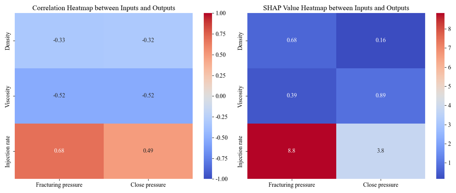
Figure 2 demonstrates that injection rate exhibits the most significant influence on fracturing pressure (P_b) and closure pressure (P_s), with a pronounced positive correlation observed, particularly for fracture pressure. In contrast, fluid density and viscosity demonstrate comparatively weaker correlations with these output parameters. Owing to the multifaceted influences on P_b and P_s – where complex interactions among governing factors may involve nonlinear relationships – conventional linear regression models may prove inadequate to accurately characterize these dependencies. To enhance predictive accuracy, this study proposes the adoption of neural network architectures or machine learning frameworks to develop error-compensated predictive models. Such approaches are anticipated to better capture the inherent nonlinear dynamics between operational variables and geomechanical responses, thereby optimizing pressure prediction fidelity in hydraulic fracturing operations.

4 MLP-KFold model

4.1 MLP model

The multilayer perceptron (MLP) model is a fully connected neural network composed of multiple neurons. By adjusting the weights of these neurons, the model minimizes prediction errors, enabling effective training and subsequent outcome prediction (Zhang et al., 2021). The MLP features a multi-layered structure, including an input layer, one or more hidden layers, and an output layer, as illustrated in the network architecture diagram (Fig. 3).

Figure 3 MLP Model Structure Diagram.

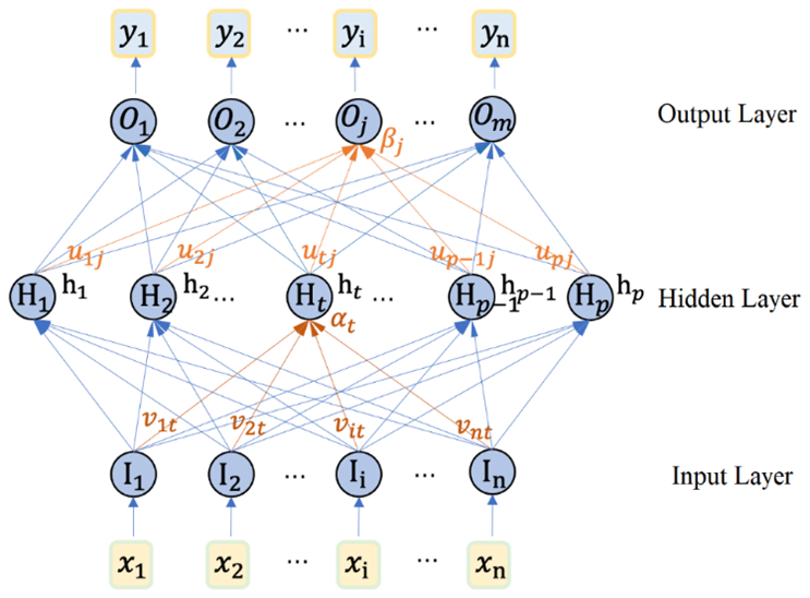
The neurons in an MLP model receive input signals, sum them with weights, and produce an output through an activation function. Building upon the perceptron model, MLP increases the nesting level of neurons and introduces an activation function between the inputs and outputs of each layer, thereby enhancing the learning capabilities of the MLP model. The output formula of a neuron is shown in Eq. (3), where σ represents the activation function.

$$\begin{array}{}\text{(3)}& y=\mathit{\sigma }\left(\sum _{i=\mathrm{1}}^n{\mathit{\omega }}_i{x}_i+b\right)\end{array}$$

And from the hidden layer to the output layer: suppose there are p neurons in the output layer, and the weight matrix from the hidden layer to the output layer is W₂. Then the output of the output layer is shown in Eq. (4), where k=1, 2, …, p. By continuously iterating and updating the weights and biases, the model can effectively fit the data and make accurate predictions.

$$\begin{array}{}\text{(4)}& {\widehat{y}}_k=\mathit{\sigma }\left(\sum _{j=\mathrm{1}}^n{W}_{\mathrm{2}kj}{h}_j+b_{\mathrm{2}k}\right)\end{array}$$

4.2 Model Structure of MLP-KFold

The MLP-KFold model combines a Multilayer Perceptron (MLP) with K-Fold Cross-validation (KFold) as a method for model training and evaluation. The MLP-KFold is built using the Sequential model, which is composed of multiple network layers stacked in sequence. The data flows through each layer in order from front to back for processing. As shown in Fig. 4, the MLP model is primarily a feedforward neural network composed of an input layer, hidden layers, a Dropout layer, and an output layer. The input layer has a dimension of 6, corresponding to the number of features in the dataset (as listed in Table 2). The three hidden layers consist of 96, 48, and 24 neurons, respectively, all using the ReLU activation function and L2 regularization to prevent overfitting. A Dropout layer is added after the first and second hidden layers to further mitigate the risk of overfitting. The output layer contains 2 neurons, corresponding to the two prediction targets: fracturing pressure (P_s) and closure pressure (P_b).

Figure 4 MLP-KFold Model Structure Diagram.

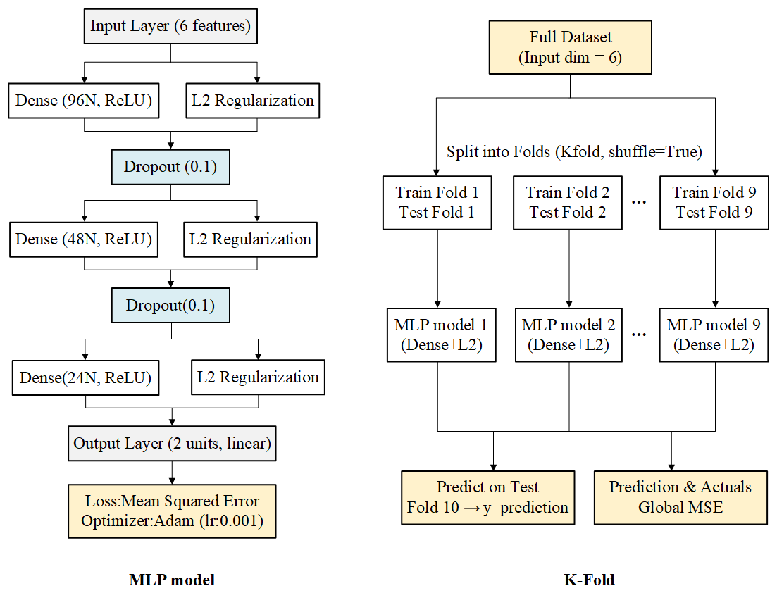
To maximize the utility of the small-scale dataset and enhance evaluation reliability, the K-Fold model adopts 10-fold cross-validation (KFold), therefore, it is suitable for the smaller scale dataset in this paper. The data is randomly split into 10 subsets – 9 for training and 1 for testing – and this process repeats 10 times, cycling through each subset as the test set. This ensures every data point contributes to validation, leading to a more robust and stable performance assessment.

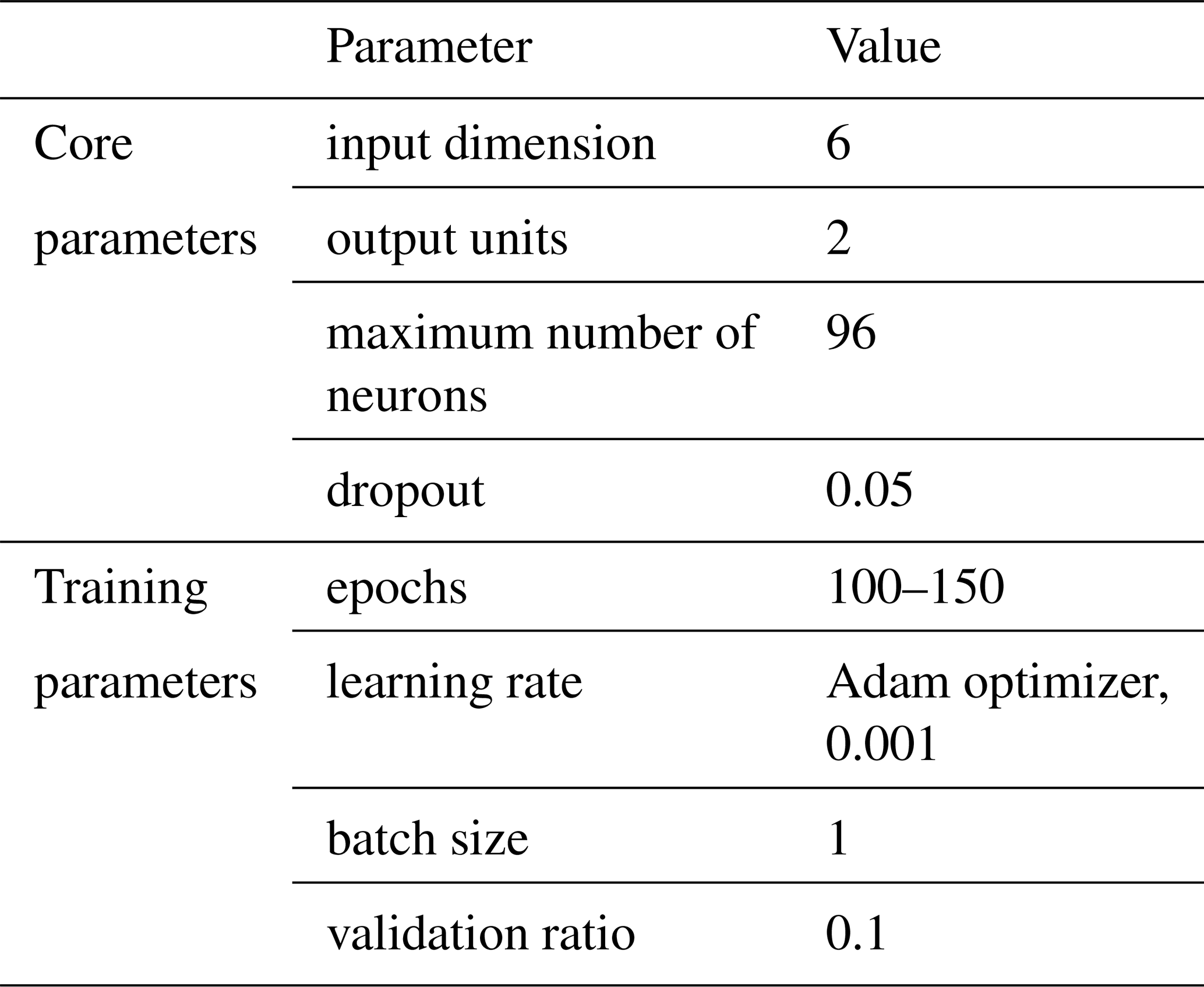
4.3 Parameter Setting

The core and training parameters of the MLP-KFold model are systematically configured prior to model implementation. The core parameters include: input dimension, output units, maximum number of neurons, and dropout. The training parameters include: number of epochs, learning rate, batch size, and validation ratio, as detailed in Table 3. Following parameter initialization, the model was trained using the prepared training dataset through iterative optimization processes.

Table 3 Parameter Setting Table.

5 Discussion

5.1 The prediction performance of MLP KFold

Following the model architecture and parameter configuration detailed in Sect. 3, the machine learning model was trained using the specified training dataset (refer to Table 4). The training process enables the model to learn inherent patterns and characteristic features within the data, thereby establishing predictive capabilities for subsequent correction and forecasting applications. Post-training visualization analysis revealed the comparative performance between actual and predicted values for both fracture pressure and closure pressure, as illustrated in Fig. 5. In this graphical representation, blue bars denote measured pressure values while red bars indicate model-predicted values, demonstrating the algorithm's predictive accuracy through visual comparison of these dual pressure parameters.

Table 4 Performance indices of the MLP-KFold model.

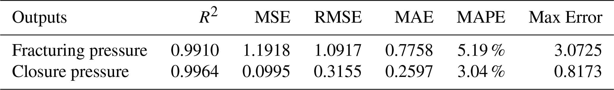
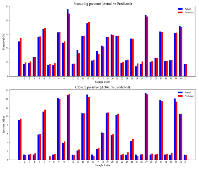
Figure 5 Comparative performance between actual and predicted values for both fracture pressure and closure pressure.

As evidenced in Table 4, the MLP-KFold model demonstrates exceptional predictive accuracy, achieving a mean R² coefficient of determination of 0.9937 – a value remarkably close to the ideal unity. The error metrics further substantiate this performance, with the Mean Absolute Percentage Error (MAPE) and Mean Squared Error (MSE) registering at minimal values of 4.115 % and 0.6457 respectively. Notably, the maximum observed prediction error remains constrained to 1.9449 MPa, confirming tight error distribution boundaries. These collective findings indicate that the proposed model successfully accounts for 99.37 % of total data variance, achieving near-perfect goodness-of-fit. The minimal divergence between predicted values and empirical observations validates the model's robust generalization capabilities across the experimental dataset.

5.2 Multi-model comparative analysis

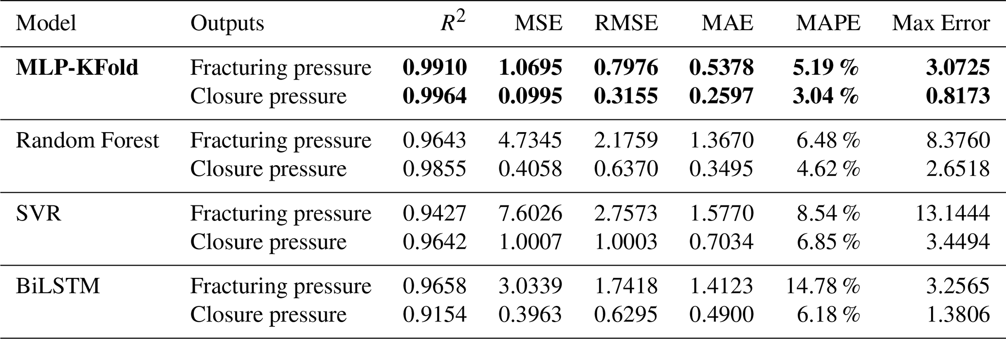
Based on the satisfactory fitting performance achieved by the MLP-KFold model, a systematic comparison study is subsequently conducted to evaluate its predictive efficacy against alternative machine learning architectures, including Random Forest (ensemble-based decision tree model), Support Vector Regression (SVR, kernel method), and Bidirectional Long Short-Term Memory (BiLSTM, deep sequential learning framework). This benchmarking framework employs identical training datasets and preprocessing protocols to ensure fair performance assessment. Quantitative metrics such as mean squared error (MSE) and coefficient of determination (R²) will be comparatively analyzed across all models, while their generalization capabilities and computational efficiency will be critically examined. The cross-model comparison aims to (1) validate the robustness of MLP-KFold in handling geomechanical pressure prediction tasks, (2) identify algorithm-specific advantages under controlled experimental conditions, and (3) establish methodological guidelines for optimal model selection in fracture pressure characterization studies. Table 5 shows performance indices of the multi-model.

Table 5 Performance indices table of the multi-model. The bold font represents MLP KFold.

The radar chart of error indices is plotted using Z-score normalization to provide a more intuitive visualization of the performance of different models across various error indices, facilitating model comparison and evaluation. Since five error coefficients from Table 5 needed to be compared simultaneously, Z-score standardization is applied to effectively mitigate the influence of scale differences and outliers in the radar chart.

Figure 6 Comparison chart of evaluation indices of the multi-model.

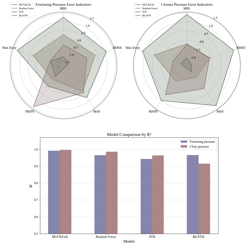
In the context of small-scale datasets, Fig. 6 shows that selecting an appropriate model is critical, as limited data inherently increases the risk of model overfitting and reduces generalization capability. MLP-KFold demonstrates robust performance when applied to small-scale hydraulic fracturing simulation datasets, and its effectiveness can be attributed to the following aspects:

1. Cross-validation mechanism: The K-fold cross-validation integrated in MLP-KFold enables full utilization of limited data, thereby enhancing model generalization and mitigating overfitting risks. By iteratively partitioning the dataset into training and validation subsets, this approach ensures reliable performance evaluation while maximizing data exploitation.

2. Simplified model architecture: As a relatively simple neural network structure, the Multilayer Perceptron (MLP) inherently requires fewer data samples to achieve stable convergence compared to complex deep learning architectures. This characteristic makes MLP particularly suitable for small-scale datasets where intricate pattern learning is constrained by data scarcity.

3. Regularization integration: MLP-KFold systematically incorporates regularization techniques, including L2 regularization and Dropout, to further suppress overfitting tendencies. These mechanisms impose constraints on weight optimization and randomly deactivate neurons during training, effectively reducing model complexity and enhancing robustness to noise in limited data scenarios.

This combination of methodological advantages positions MLP-KFold as a computationally efficient and statistically reliable framework for analyzing small-scale experimental datasets in hydraulic fracturing simulations.

Table 6 Comparison table of hydraulic fracturing in-situ stress measurement results.

5.3 Model Generalization Capability

While the MLP-KFold model demonstrated remarkable performance on the test set with a coefficient of determination (R² = 0.9937), it is acknowledged that the diversity of rock types, formation conditions, and construction parameters in real-world applications could pose challenges to the model's generalization capability. To further validate the model's robustness and adaptability across different geological environments and construction scenarios, the following aspects should be discussed.

1. Cross-Validation with diverse datasets: by merging cross-validation with datasets spanning various geological settings and construction conditions with field trials in multiple locations, we can comprehensively assess the model's performance in real-world applications. This integrated method not only identifies potential weaknesses or biases in the model but also provides empirical data from different geological environments, thereby enabling targeted adjustments to improve generalization.

2. Incorporation of additional features: to further bolster the model's adaptability, we advocate for the incorporation of additional features that encapsulate the variability in geological and construction parameters. These features may encompass rock anisotropy, formation fluid properties, and dynamic construction variables, among others. In parallel, establishing a framework for continuous model updating based on new data and feedback from field applications ensures the model evolves with emerging geological and construction challenges, maintaining its accuracy and relevance.

In summary, these strategies aim to enhance the model's generalization capability and reliability across a broad spectrum of practical applications. Future efforts will concentrate on expanding the dataset, conducting extensive field trials, and refining the model to address the intricacies of real-world hydraulic fracturing operations.

6 Engineering application

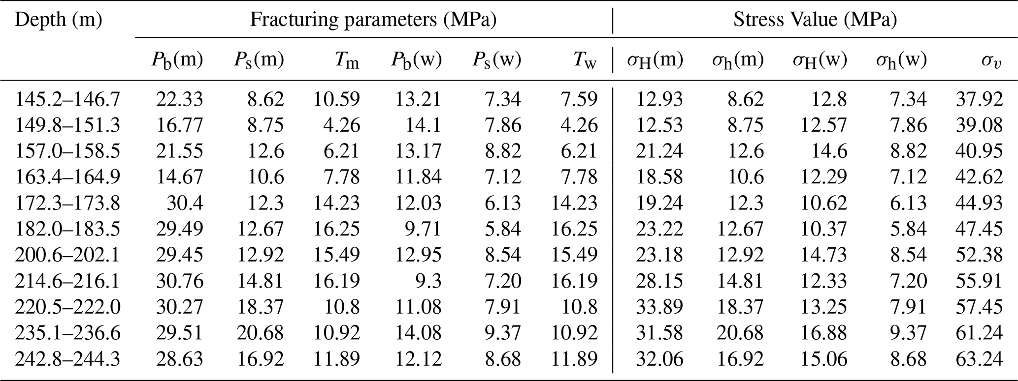
The MSZK and ZPZK boreholes are serving as adjacent boreholes for in-situ stress testing within a hydraulic investigation and design project, both boreholes were designed to a depth of 275 m, with hydraulic fracturing in-situ stress measurements conducted following standardized operational procedures (Zhang, 2018). A total of 11 fracturing intervals were implemented within the depth range of 145.2–244.3 m across both boreholes, with key fracturing parameters and results summarized in Table 7. The MSZK maintained favorable wellbore conditions, enabling the use of clean water as fracturing fluid. In contrast, the ZPZK required drilling mud (density: 1.5 g cm⁻³, viscosity: 235 mPa s) for wall stabilization due to severe borehole collapse. A comparative analysis of hydraulic fracturing stress measurement outcomes between MSZK and ZPZK under distinct fracturing fluid conditions is presented in Table 6, demonstrating significant differences in in-situ stress measurement outcomes attributable to fluid medium variations.

Here, P_b(m): ZPZK fracturing pressure by mud; P_s(m): ZPZK closure pressure by mud; T: rock tensile strength; P_b(w): MSZK fracturing pressure by water; P_s(w): MSZK closure pressure by water; σ_H(m): ZPZK maximum horizontal principal stress; σ_h(m): ZPZK minimum horizontal principal stress; σ_H(w): MSZK maximum horizontal principal stress; σ_h(w): MSZK minimum horizontal principal stress; σ_v: vertical principal stress (the overburden rock unit weight was assigned as 26.5 kN m⁻³).

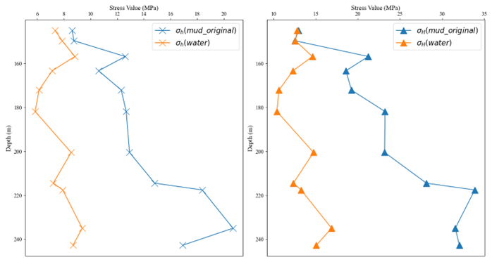
Figure 7 Comparative curves of maximum and minimum horizontal principal stresses between ZKZP(mud) and MSZK(water).

Table 7 Comparison table of hydraulic fracturing in-situ stress measurement results after compensation.

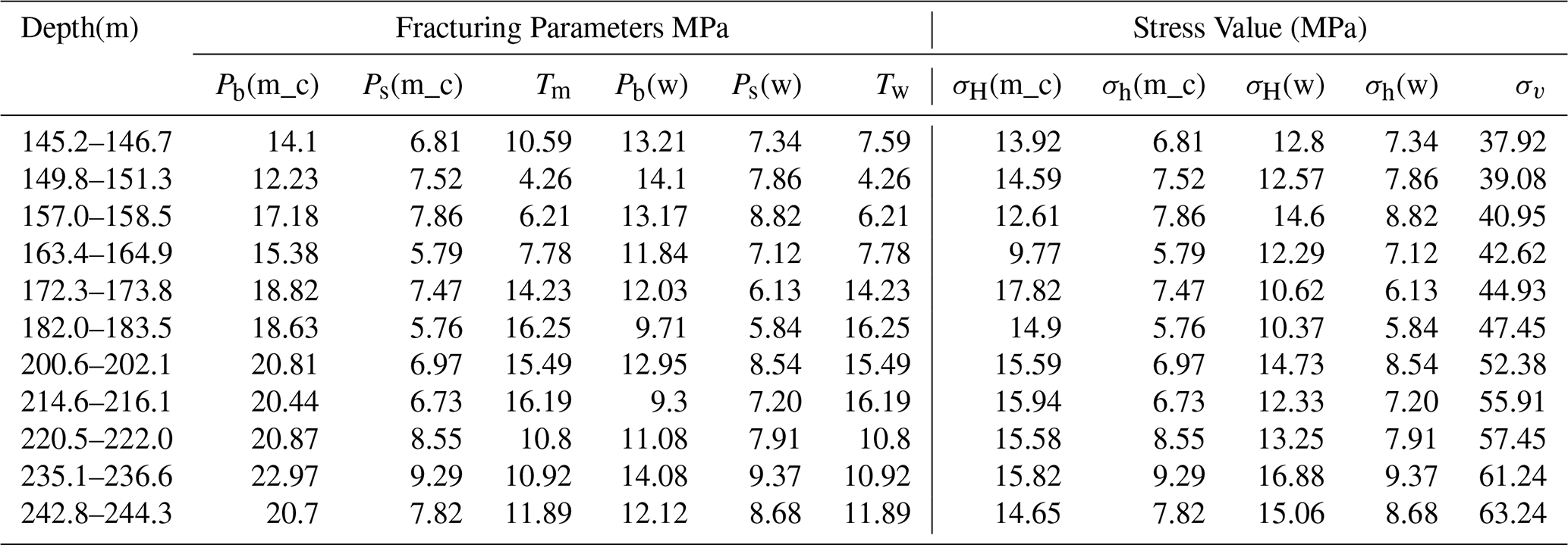
Figure 7 demonstrates the comparative curves of maximum and minimum horizontal principal stresses between ZKZP(mud) and MSZK(water). The analysis reveals significantly higher in-situ stress calculation results for ZKZP compared to MSZK. The average percentage differences reach 39.32 % for maximum horizontal principal stress and 39.61 % for minimum horizontal principal stress within equivalent depth intervals. Considering the close proximity of these two boreholes (only 50 m apart) and their comparable geological conditions with identical lithological characteristics in surrounding strata, this substantial discrepancy strongly suggests that the drilling mud medium in boreholes exerts considerable influence on measurement outcomes such as rock breakdown values. To address this systematic bias, the MLP-KFold model was subsequently employed to calibrate critical output parameters (fracture pressure and closure pressure values). The refined in-situ stress calculation results after correction are presented in Table 7.

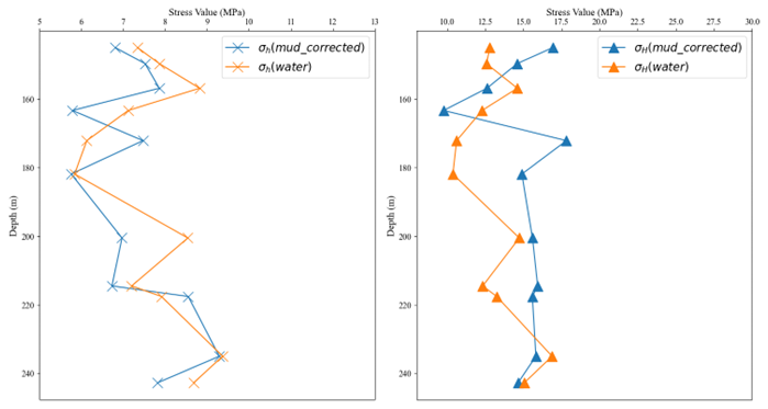
Figure 8 The comparative curves of maximum and minimum horizontal principal stresses between the calibrated ZKZP and MSZK.

Here, (m_c) represents the pressure value of mud as the fracturing fluid after the MLP-KFold correction. The comparative curves of maximum and minimum horizontal principal stresses between the calibrated ZKZP and MSZK are presented in Fig. 8. As illustrated in Fig. 9, the discrepancy in calculated in-situ stress values between the two boreholes shows a marked reduction after model calibration. Within equivalent depth intervals, the maximum horizontal principal stress difference decreases to 17.84 %, while the minimum horizontal principal stress difference demonstrates a more pronounced improvement, achieving a remarkable decrease to 10.58 %.

7 Conclusions

This paper presents a rock mechanics measurement result correction model based on MLP KFold, developed from a dataset constructed via hydraulic fracturing simulation experiments. The model demonstrates superior performance in addressing measurement deviations of hydraulic fracturing-induced fracture and closure pressures, enhancing the accuracy of in-situ stress calculations. By combining MLP with K-Fold cross-validation, this study offers a data-efficient solution for in-situ stress measurement correction and optimizing regional stress profile assessments. The key findings are as follows:

1. The MLP KFold model shows outstanding predictive ability on small-scale datasets, achieving an R² of 0.9937, surpassing benchmark models by Δ+1.89 %–+5.34 %, and its low error metrics (MAE = 0.518, MSE = 0.646, and maximum error = 1.945 MPa) confirm its predictive accuracy and robustness with limited experimental data.

2. The model significantly reduces average discrepancies in principal stress calculations under varying fracturing fluid conditions (σ_H: −21.48 %; σ_h: −29.03 %), effectively addressing errors from fracturing fluid property differences. This validates its engineering applicability and effectiveness in hydraulic fracturing stress measurements under complex field conditions.

Appendix A

Table A1 Optimal design table of values for the hydraulic fracturing simulation experiments.