A new magnetic observatory in La Réunion Island – meeting data quality requirements in a volcanic island setting

A new magnetic observatory has been set on La Réunion Island in the Indian Ocean through a collaboration between the “Institut de physique du globe de Paris” (IPGP) local volcano observatory (Observatoire Volcanologique du Piton de la Fournaise – OVPF) and its magnetic observatory service. This observatory is isolated and serves to monitor the evolution of the Earth's magnetic field in that region. It is also particularly useful for large-scale modelling of the core field and other contributions to the geomagnetic field. Three-component vector magnetic field data are continuously collected at 1 Hz using a fluxgate, while scalar data are collected at 0.2 Hz with a proton magnetometer. The data are transmitted every 5 min to IPGP main site and made immediately available to the scientific community (see http://www.bcmt.fr, last access: 22 August 2025). Due to the strong magnetic field generated by the surrounding volcanic rocks, the differences between the magnetic field strengths as recorded by the proton magnetometer and the strengths calculated from the recorded vector field values vary by more than ∼2 nT during a day. To circumvent this difficulty, constant offset values of −2400, 280, and −20 nT are added to the X, Y, and Z magnetic field components respectively, prior to the data distribution. We show that this approach efficiently reduces the differences between measured and calculated magnetic field strengths inside a day. Calibrated observatory data have been calculated over the year 2023, and, although the baseline values present variations up to 70 nT throughout that year, the derived data meet the quality required for an intermagnet observatory. A Fourier analysis of the data shows that these are not contaminated by significant noise even if peaks at 0.2 Hz indicate small cross-talk between vector and scalar instruments.

1 Introduction

There are currently around 120 magnetic observatories around the world collecting data, most of them being part of intermagnet (Love and Chulliat, 2013), an international organization promoting high-quality standards for magnetic data acquisition processes and free data distribution (http://www.intermagnet.org, last access: 22 August 2025). These observatories allow the geomagnetic field changes to be monitored over decades and are utilized for the study of not only the core magnetic field but also the fields generated in the ionosphere and magnetosphere, together with those generated by their induced counterpart currents in the conductive bodies inside the Earth. Numerous other natural sources contribute to the observed magnetic data, such as oceanic tides and currents. However, to obtain a global view of the magnetic field evolution, it is preferable to have a homogeneous distribution of observatories around the world (e.g. Langel et al., 1995). This is far from being the case, with most of observatories being located in Europe and North America, while only few observatories are located in the Middle East regions, Africa, and South America. Despite very difficult climatic conditions, there are several observatories in Antarctica in contrast with oceanic areas, where only a few observatories are set on remote islands.

In the Indian Ocean, as in the Atlantic or Pacific oceans, there are currently very few observatories (see Fig. 1). To the east, Gingin (gng), Learmonth (lrm), and Cocos Island (cki) intermagnet observatories, all under Australian institution responsibilities, are producing data. To the north, India is running several intermagnet observatories: Alibag (abg), Hyderabad (hyb), and Choutuppal (cpl). There is also the Gan International Airport observatory (gan) in the Maldives that began operation in 2012. The observatory in Antananarivo (tan) stopped producing calibrated data in December 2007. A new observatory has been opened in Fihaonana (Madagascar) but is not yet distributing data. Further to the west, data were distributed by the Maputo (lmm) and Nampula (nmp) observatories in Mozambique up to 2017 and 2019, respectively, and by Hartebeesthoek (hbk) observatory. To the south, three observatories on the Kerguelen, Crozet, and Amsterdam islands have not been delivering calibrated data to Edinburgh World Data Center (wdc.bgs.ac.uk) since 2013, 2015, and 2013, respectively, although there is some variation (i.e. non-calibrated), data are available on the bcmt data repository (http://www.bcmt.fr, last access: 22 August 2025). To enhance the spatial coverage of observatories in the central Indian Ocean, a new observatory was established on La Réunion Island, approximately 875 km to the east of the former Antananarivo observatory and more than 1800 km away from the closest currently active observatory in Nampula (Mozambique). The choice of this island comes primarily from the predicted evolution of main magnetic field given by the International Geomagnetic Reference Field, version 13 (igrf-13), which forecasts a maximum increase in the Southern Hemisphere magnetic field strength in this area. Besides, the “Institut de physique du globe de Paris” (ipgp) already runs a volcanic observatory in La Réunion to monitor the Piton de la Fournaise volcano. The scientists and technicians of the volcanic observatory aided in the installation of the magnetic observatory and furthermore provide the required scientific and technical expertise to perform the weekly manual absolute measurements. The presence of the magnetic observatory on this island is also a new asset for processing magnetic survey or variometer station data acquired for monitoring the volcano activity.

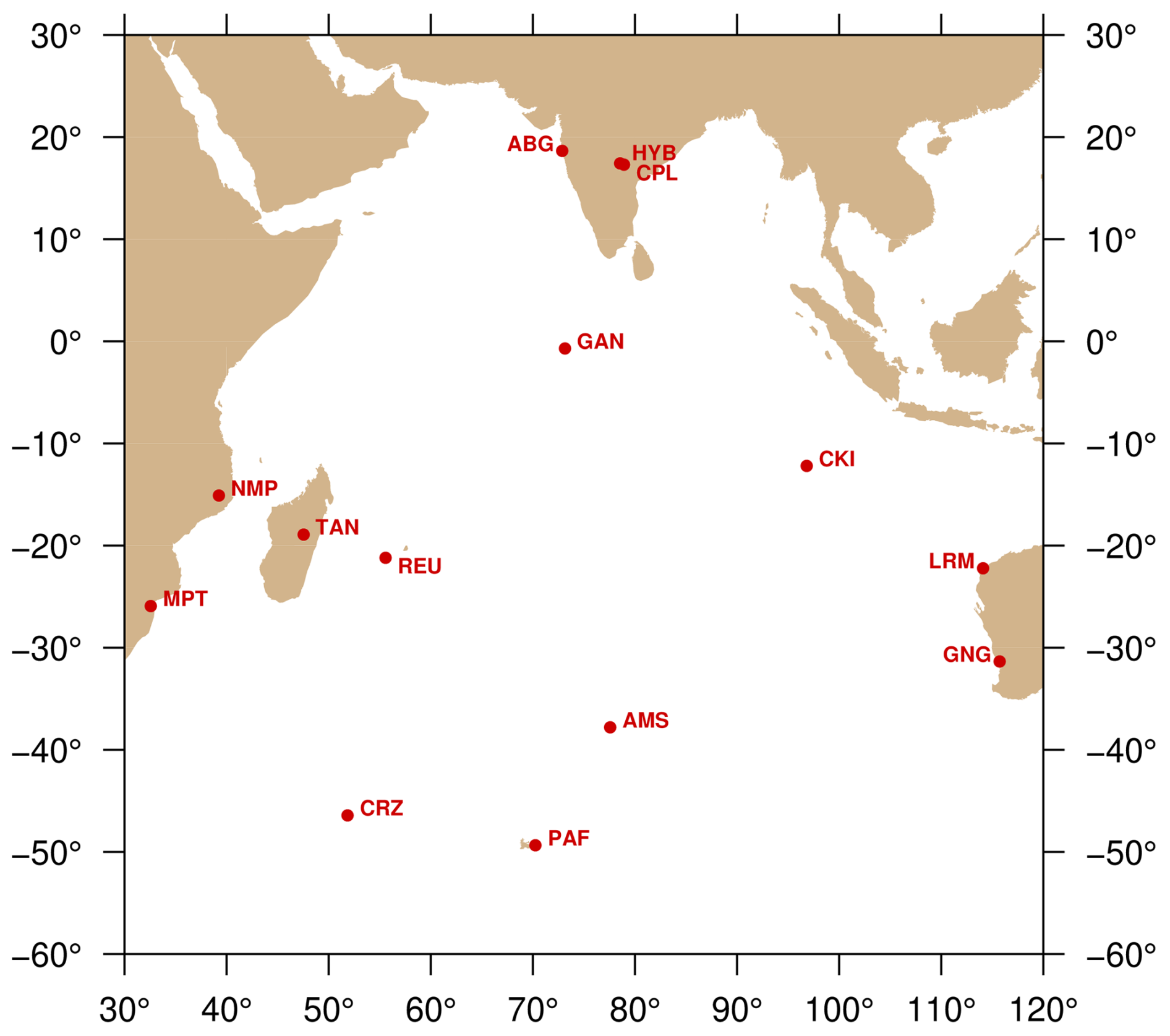
Figure 1 Map of magnetic observatories in the Indian Ocean that have released data in recent years.

Building an observatory on an isolated island usually comes with specific challenges as these islands are typically of volcanic origin and therefore are made of rocks presenting strong magnetization. It follows that, contrary to the traditional continental setup, observatories on these islands are often located in areas of strong magnetic field gradients. Such gradients do not preclude accurate measurements of the magnetic field strength and direction when modern instruments are used, but it is nonetheless difficult to reconcile the data acquired at different locations of the observatory site. These data are continuous series of vector magnetic field measurements made using fluxgate magnetometers, series of total field strength generally obtained with a proton or optically pumped absolute magnetometer, and manual absolute measurements typically made on a weekly basis. These three types of data are measured at different places, a few metres apart, and have to be processed to give a continuous series of calibrated vector magnetic data located on the absolute reference pillar of the observatory. It is this continuous series of second- or minute-mean calibrated data that is ultimately distributed by the observatories for scientific or technical applications.

In the next section the new observatory location and setting are described in detail. In Sect. 3 the data processing applied on the vector data to estimate the field on the observatory reference pillar is presented. In the following section results of 1 full year of data acquisition are shown. Calibrated data for the year 2023 are presented and analysed. The last section is dedicated to the conclusion.

2 La Réunion observatory setting

La Réunion Island, located in the Indian Ocean, is a volcanic island characterized by strong magnetic anomalies and steep gradients due to highly magnetized rocks. Several sites were considered for setting the magnetic observatory in the “Plaine des Caffres”, a smooth and relatively flat area, south of the island, between the two volcanoes. Aeromagnetic surveys conducted over the area indicated relatively low gradients in the area. To refine site selection, we carried out both vertical and horizontal gradient surveys at candidate locations. The resulting grid maps and spot measurements of the total magnetic field revealed the heterogeneous nature of the volcanic magnetic environment, highlighting the challenges inherent in establishing an observatory in such a setting. The observatory installation was completed within 1 year in three main stages: surveys of potential sites, pillar construction, and equipment deployment. The chosen site at 21°12^′21.2^′′ S, 55°34^′35.3^′′ E, and 1580 m altitude, is as isolated as possible and situated 500 m from the volcanic observatory, where observers trained for absolute measurements and basic maintenance are available. The land, covered by forest, is owned by the national forestry office. A 9-year agreement has been signed between our institutes. The installation needed to be as little intrusive as possible but autonomous. The area has little elevation change, the forest is not dense, and no endemic trees are present, allowing us to clear the surrounding vegetation to guarantee the sun exposition of solar panels. A visual target was installed on a single concrete pole for geographical reference at a distance of about 40 m from the observatory main pillar. As secondary target, a natural peak on the volcano around 5 km away, is used. A good grounding to avoid lightning strikes and a solidly built infrastructure to provide good resistance to hurricanes have been necessary. The constructions are free from ferromagnetic (or magnetic) materials. Materials were tested using a magnetometer before use or installation. Fibre-reinforced concrete was used in place of the usual iron-reinforced concrete.

Three types of data are collected at the observatory site:

• Variation vector magnetometer data. The vector magnetic field is sampled at 1 Hz, using a dvm-19 full-range three-axial fluxgate instrument built in the Chambon-la-forêt French national observatory. This instrument has a relatively low noise level (< 15 $\mathrm{pT}{\mathrm{Hz}}^{-\mathrm{1}/\mathrm{2}}$) and can be rigorously calibrated thanks to its full-range (±70 µT) capabilities. It has, as all fluxgate instruments, a dependence on temperature that is of the order of 300 pT °C⁻¹. The instrument is seated on the “variometer” pillar; because of possible movements of the pillar or slight temperature variations, the collected data cannot be seen as absolute data. The data collected form the variation vector data.

• Variation scalar magnetometer data. The scalar instrument is a Geomag SM90R, Overhauser-type, scalar absolute magnetometer sampling the magnetic field at 0.2 Hz. These types of instruments are sensitive to magnetic field gradients; therefore, the scalar magnetometer was installed at a height of 1.7 m above the ground and positioned several metres away from the vector magnetometer. This setup minimizes potential interference between the two instruments. These types of data are called the variation scalar data.

• Manual absolute measurements. The manual absolute data are collected on the observatory main pillar using a Bartington Mag01H single-axis fluxgate magnetometer probe mounted on a Zeiss 010A non-magnetic theodolite. Each absolute observation is a combination of a series of eight manual declination and inclination measurements. These angle measurements are completed with absolute measurements of the magnetic field strength made using a Gemsystem GSM-90T. The technique used has been described for example in Newitt et al. (1996). These types of data are collected at least once a week.

As partly described above, two pillars made of fibre reinforced concrete were built to position the instruments: a large and deep one, at chest height – i.e. 1.4 m, for absolute measurements and, ∼10 m away, a small one on which to rest the variation vector magnetometer. This latter variometer pillar is ∼40 cm above ground and is covered by a well-insulated box, filled with water bottles for increased temperature stability. Such a short pillar means increased measurements stability over long time periods. However, it also means larger contributions from magnetized surrounding rocks. Our choice of a short pillar is due to the risk associated with recurrent hurricanes in this region and therefore to the requirement of a robust installation. This study demonstrates the methods employed to mitigate the influence of strong magnetic contributions from surrounding rock formations. The variation scalar magnetometer sits on a 1.7 m tall mast, fixed in concrete and covered in a PVC tube. This variometer pillar, the variation scalar magnetometer site, and their respective electronics are roughly 6 m from each other, forming a triangle shape (see plan in Fig. 2). Vector and scalar data are acquired by an IPGP in-house built “ENO4” data logger, which is based on a BeagleBone platform, and transmitted to the Paris main servers via GSM digital cellular signal, typically every 5 min. A mqtt real-time transmission protocol is integrated and used for monitoring purpose. The observatory has been designed to require low electric power and to be autonomous in power and communication, with a single solar panel and a GSM transmitter placed 25 m away from the sensors.

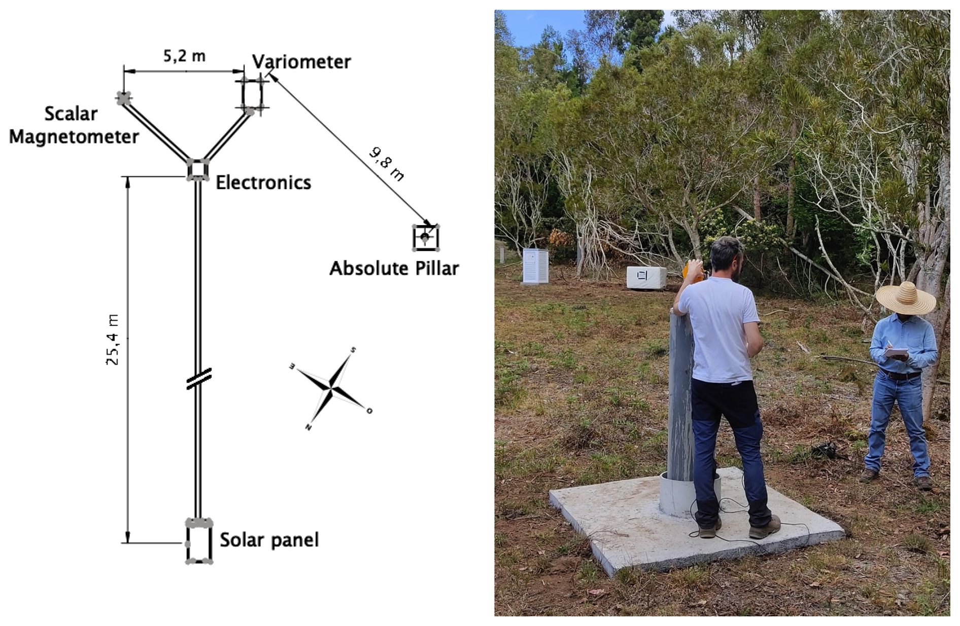
Figure 2 Left: a schematic map of the observatory. Right: photograph showing the layout of the La Réunion Observatory. In the foreground, the main observatory pillar is seen during a training session. In the background, from left to right, are the grey concrete target pole; the white meteorological box housing the sensor electronics; the grey vertical PVC tube, partially obscured by trees, containing the variation scalar magnetometer; and the plastic box containing the variation vector magnetometer, covered with a white thermal blanket.

Variation data and absolute measurements started in December 2022. The island is subject to seasonal hurricanes/tropical cyclones, but the observatory did not suffer as a result of Hurricane Belal on 15 January 2024. Only the GSM connection was down for a few days. There are no frequent thunder strikes in the area. We do not foresee major difficulties in the operation of this observatory regarding its general infrastructure over the coming decade.

3 Data processing

3.1 Variation data and processing technique

The calibrated data distributed by the observatory are series of 1 Hz variation vector magnetic data and 0.2 Hz variation scalar data but estimated on the observatory main pillar (or main pillar) site such that they fit the manual measurements. The differences between the magnetic field strengths computed from the variation vector measurements and variation scalar data, as estimated on the main pillar, define a data quality criterion. These differences are expected to stay within ∼1 nT around zero to meet the intermagnet quality standard (intermagnet, 2020).

In the specific case of observatories installed in an area of strong magnetic gradient, these criteria are particularly difficult to meet, even for time series of less than a day for which the pillars can be assumed to be steady and temperature variations to be negligible. Let us assume that the magnetic field at the variometer pillar is

$$\begin{array}{}\text{(1)}& {\mathit{b}}_{\mathrm{v}}=\left[\begin{array}{c}{x}_{\mathrm{v}}\\ y_{\mathrm{v}}\\ z_{\mathrm{v}}\end{array}\right],\end{array}$$

where x_v , y_v, and z_v are the three magnetic field orthogonal components in the magnetometer reference frame – i.e. the frame defined by the three orthogonal axis of the fluxgate magnetometer. The associated magnetic field strength is

$$\begin{array}{}\text{(2)}& F_{\mathrm{v}}=\sqrt{x_{\mathrm{v}}^{\mathrm{2}}+y_{\mathrm{v}}^{\mathrm{2}}+z_{\mathrm{v}}^{\mathrm{2}}},\end{array}$$

but the strength of the field on the observatory main pillar is

$$\begin{array}{}\text{(3)}& F_{\mathrm{p}}=\sqrt{(x_{\mathrm{v}}+\mathit{\delta }x{)}^{\mathrm{2}}+(y_{\mathrm{v}}+\mathit{\delta }y{)}^{\mathrm{2}}+(z_{\mathrm{v}}+\mathit{\delta }z{)}^{\mathrm{2}}},\end{array}$$

where δx, δy, and δz are the differences in the magnetic vector field on the main pillar relative to the field recorded on the variometer pillar, in the same reference frame. It can be assumed that these differences are constant in time, which is consistent with the assumption that the magnetic field gradient observed on site is exclusively due to the magnetization of local rocks and is not linked to external, induced or core field signals. It can be shown (see Appendix A) that, to the first order in perturbations, the magnetic field strength difference between the recorded magnetic field at the variometer pillar and its value on the observatory main pillar is

$$\begin{array}{}\text{(4)}& \mathrm{\Delta }F=F_{\mathrm{p}}-F_{\mathrm{v}}\simeq {\widehat{\mathit{b}}}_{\mathrm{v}}\cdot \left[\begin{array}{c}\mathit{\delta }x\\ \mathit{\delta }y\\ \mathit{\delta }z\end{array}\right],\end{array}$$

where ${\widehat{\mathit{b}}}_{\mathrm{v}}={\mathit{b}}_{\mathrm{v}}/F_{\mathrm{v}}$ is the unit vector giving the magnetic field direction at the variometer pillar site. As the magnetic field on the variometer pillar changes in direction over time – e.g. due to the S_q current system in the dayside ionosphere, it is clear that ΔF changes with time even if δx, δy, and δz are constant. The variations in ΔF over a day are generally small but cannot be neglected for observatories set in areas of strong magnetic field gradients – i.e. where the δx, δy, and δz values can reach a thousand nanoteslas (nT) or more. This is the case for La Réunion observatory, where the variometer pillar is small and therefore where the surrounding rock magnetization contributes significantly to the recorded magnetic field components (see Sect. 2). In the longer term, for example a year, ΔF may change significantly with temporal variations of δx, δy, and δz due to, for example, temperature or environmental changes.

Keeping the daily ΔF variations within small values is a prerequisite for deriving definitive calibrated data at La Réunion observatory. A simple but efficient way to solve this problem is to set up a method for estimating the δx, δy, and δz values in the sensor reference frame. This is precisely what the baseline estimation method presented in Lesur et al. (2017) does. This approach is briefly revisited in the remainder of this section.

The calibrated magnetic vector field b_p estimated on the observatory main pillar in a local geodetic reference frame is

$$\begin{array}{}\text{(5)}& {\mathit{b}}_{\mathrm{p}}={\mathbf{R}}_{\mathit{\theta }}\left[\begin{array}{c}{x}_{\mathrm{v}}+\mathit{\delta }x\\ y_{\mathrm{v}}+\mathit{\delta }y\\ z_{\mathrm{v}}+\mathit{\delta }z\end{array}\right],\end{array}$$

where R_θ is a rotation matrix for an angle θ, positive anti-clockwise, around the local vertical axis. There are four calibration parameters to be estimated, namely θ, δx, δy, and δz. We assume that θ takes a constant value over several months whereas the other parameters are taking constant values only over a single day. The vertical direction on the variometer pillar is assumed to be the same as on the main pillar. It follows that δz is independent from the θ angle, whereas the δx and δy depend strongly on this angle value. It is noted that the vector magnetic instrument is oriented such that its x component is approximately aligned with the direction of the local magnetic north, and it follows that the θ angle is close to ($-\mathrm{1}\times$) the declination angle¹ when the δx and δy parameters are small. However, that angle may be significantly different from the declination when δx and δy parameters are large – i.e. when there are local strong gradients of the magnetic field on the observatory site.

To estimate the calibration parameter values, we require the calibrated magnetic vector field to match the absolute observations obtained on the observatory's main pillar. However, this constraint alone is insufficient for a robust estimation of the angle θ. Therefore we additionally require the calibrated magnetic vector field to fit the hourly spot values of the magnetic field strength F_s given by the variation scalar data. This requires the introduction of a further parameter $\mathit{\delta }F=F_{\mathrm{p}}-F_{\mathrm{s}}$, also constant over one day, that describes the magnetic field strength difference between the main pillar position and the scalar variometer position, assuming the δF constant is only valid if the magnetic field gradients are small between these two positions. This is a reasonable approximation because the main pillar and the scalar proton magnetometer are 1.5 and 1.7 m over ground, respectively, and therefore are in an area of smaller magnetic gradients. This approximation was validated by placing an additional scalar magnetometer on the main pillar for 1 d (23 June 2023) to record, at 0.2 Hz, the magnetic field strength simultaneously at the two locations, the main pillar and the variation scalar magnetometer pillar. The difference between the measurements did not exceed 0.5 nT.

Let us assume that we have a set of absolute data on the main pillar and that a rotation angle θ is chosen; then, there are two types of equations that can be used to find the daily values of δx, δy, δz, and δF:

$$\begin{array}{}\text{(6)}& \begin{array}{l}\left[\begin{array}{c}{x}_{\mathrm{a}}\\ y_{\mathrm{a}}\\ z_{\mathrm{a}}\end{array}\right]-\left[\begin{array}{c}{\stackrel{\mathrm{̃}}{x}}_{\mathrm{v}}\\ {\stackrel{\mathrm{̃}}{y}}_{\mathrm{v}}\\ {\stackrel{\mathrm{̃}}{z}}_{\mathrm{v}}\end{array}\right]={\mathbf{R}}_{\mathit{\theta }}\left[\begin{array}{c}\mathit{\delta }x\\ \mathit{\delta }y\\ \mathit{\delta }z\end{array}\right]+\left[\begin{array}{c}{\mathit{ϵ}}_x\\ {\mathit{ϵ}}_y\\ {\mathit{ϵ}}_z\end{array}\right],\\ \\ \text{where}\left[\begin{array}{c}{\stackrel{\mathrm{̃}}{x}}_{\mathrm{v}}\\ {\stackrel{\mathrm{̃}}{y}}_{\mathrm{v}}\\ {\stackrel{\mathrm{̃}}{z}}_{\mathrm{v}}\end{array}\right]={\mathbf{R}}_{\mathit{\theta }}\left[\begin{array}{c}{x}_{\mathrm{v}}\\ x_{\mathrm{v}}\\ x_{\mathrm{v}}\end{array}\right],\end{array}\end{array}$$

and

$$\begin{array}{}\text{(7)}& F_{\mathrm{s}}-F_{\mathrm{v}}={\widehat{\mathit{b}}}_{\mathrm{v}}\cdot \left[\begin{array}{c}\mathit{\delta }x\\ \mathit{\delta }y\\ \mathit{\delta }z\end{array}\right]-\mathit{\delta }F+{\mathit{ϵ}}_{\mathrm{s}},\end{array}$$

where x_a, y_a, and z_a are the three components in a geodetic reference frame of the magnetic field vector derived from the manual absolute measurements of the declination, inclination, and total field strength on the main pillar of the observatory. ϵ_x, ϵ_y, ϵ_z, and ϵ_s are the errors that should reduce to measurement errors once the δx, δy, δz, and δF values have been adjusted. ϵ_s includes also the errors associated with the linearization in Eq. (4).

The variances of the errors in the right-hand side of Eqs. (6) and (7) are minimized iteratively by adjusting δx, δy, δz, and δF, where the iterations combined with a classic re-weighting least-squares approach allow the weak non-linearity in Eq. (7) to be handled as well as the possible non-Gaussian distributions of residuals (see, for example, Farquharson and Oldenburgh, 1998). We observe that the quality of the fit to the data depends heavily on the chosen θ angle value.

3.2 Application to La Réunion observatory data

The first step required to process the data is to choose the θ angle. For this, we prepared a dataset that includes manual absolute measurements x_a, y_a, and z_a and the total intensity measurements F_s sampled every 2 h, from 1 January to 7 June 2023. The dataset is shown in Fig. 3. Absolute data can be compared with variation vector data at the same instant, indicating large magnetic gradients on the observatory site, although the reference frames for the variation vector data and the absolute data are different. The magnetic field strength differences F_v−F_s are of the order of 675 nT; variations can exceed 2 nT during a single day.

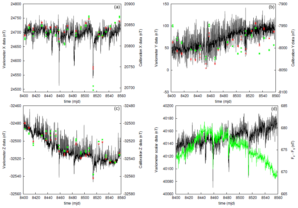
Figure 3 Datasets: (a, b) X and Y components and (c, d) Z component and total intensity data. The time unit is “modified Julian day” (mjd) – i.e. decimal day number starting from 1 January 2000 at 00:00 UT. Variation data decimated to one point every 2 h are shown in black, and variation data at the reference times corresponding to the absolute data are shown in red. Scales are on the left-hand side of the figures. The absolute data for the X, Y, and Z components and F_v−F_s for the total intensity data are shown in green. Scales are on the right-hand side of the figures. The X and Y axis of the absolute data are in the geodetic reference frame but are in the instrument reference frame for variation vector data.

Our ability to minimize the left-hand side of Eqs. (6) and (7), by adjusting the δx, δy, δz, and δF values, has been tested for θ values in the range [0:45]°. Results are shown in Fig. 4, where the misfits for the horizontal, vertical, and total intensity are defined by

$$\begin{array}{}\text{(8)}& \begin{array}{l}{M}_H=\sqrt{\sum _{\mathit{\left\{}i\mathit{\right\}}}({\mathit{ϵ}}_{xi}^{\mathrm{2}}+{\mathit{ϵ}}_{yi}^{\mathrm{2}})/{\mathit{\sigma }}_i^{\mathrm{2}}},\\ M_Z=\sqrt{\sum _{\mathit{\left\{}i\mathit{\right\}}}{\mathit{ϵ}}_{zi}^{\mathrm{2}}/{\mathit{\sigma }}_i^{\mathrm{2}}},\\ M_F=\sqrt{\sum _{\mathit{\left\{}i\mathit{\right\}}}{\mathit{ϵ}}_{si}^{\mathrm{2}}/{\mathit{\sigma }}_i^{\mathrm{2}}},\end{array}\end{array}$$

respectively, where the errors ϵ_xi, ϵ_yi, ϵ_zi, and ϵ_si are defined in Eqs. (6) and (7), and ${\mathit{\sigma }}_i^{\mathrm{2}}$ denotes the expected variances of the corresponding errors. The quantities M_H, M_Z, and M_F in Eq. (8) are unitless, and the summations are over all available absolute measurements. Figure 4 shows that the smallest misfit to the data can be achieved for θ=22.0°. For this angle, the values of δx, δy, δz, and δF, as estimated with the approach described in Sect. 3.1, range in the intervals $[-\mathrm{2402}:-\mathrm{2391}]$, [322:366], $[-\mathrm{21}:-\mathrm{8}]$, and $[-\mathrm{715.5}:-\mathrm{713.2}]$ nT, respectively. These ranges are large, particularly for δy and δz. This occurs because we used an L₂ norm minimizing process that does not down-weight outliers. It is however obvious that the ΔF variations inside a day, defined by Eq. (4), are due to the very large δx values.

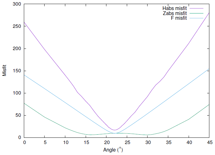
Figure 4 Misfits to data as a function of the θ rotation angle. The misfits for the horizontal component are shown in purple, misfits for the vertical component in green, and misfits for the total intensity in blue. The misfit definitions are given in Eq. (8).

In order to produce near-real-time data with ΔF values nearly constant over a day, we decomposed the process leading to calibrated data values for this observatory in two steps:

1. Apply a first correction with δx₁, δy₁, δz₁, δF₁, and θ₁ values, constant over a year, in near-real time. These data are distributed 5 to 10 min after acquisition as observatory variation data.

2. Apply a second correction with δx₂, δy₂, δz₂, and δF₂ varying from day to day but being constant over a day. The value of θ₂ remains constant over the full year and is, for 2023 and 2024, such that ${\mathit{\theta }}_{\mathrm{1}}+{\mathit{\theta }}_{\mathrm{2}}=\mathrm{22}\mathit{°}$. These calibrated data are distributed in the following year as observatory definitive data.

The offset values δx₁, δy₁, δz₁, and δF₁ can be set arbitrarily, but in order to have ΔF variations that remain small over a day, they should have values close to the δx, δy, δz, and δF intervals given above. We use

$$\begin{array}{}\text{(9)}& \begin{array}{ll}\mathit{\delta }{x}_{\mathrm{1}}=-\mathrm{2400}\mathrm{nT}& \mathit{\delta }{y}_{\mathrm{1}}=\mathrm{280}\mathrm{nT}\\ \mathit{\delta }{z}_{\mathrm{1}}=-\mathrm{20}\mathrm{nT}& \mathit{\delta }{F}_{\mathrm{1}}=\mathrm{0}\mathrm{nT}\end{array}\end{array}$$

for an angle value θ₁=0.95°. This latter value has been set arbitrarily but controls the values obtained for δx₁ and δy₁. To illustrate the effect of step (i) the bottom-right image of Fig. 3 is shown again in Fig. 5 but with the offsets applied to the variation vector data. Typical values of the magnetic field strength differences F_v−F_s have changed from around 675 to −713 nT, and although overall variations have a similar trend and amplitude, it is clear that short-term variations have been drastically reduced within a day.

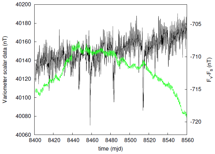
Figure 5 Total intensity values sampled every 2 h are shown in black (left scale), and in green F_v−F_s (right scale) where the rotation and offsets given in Eq. (9) have been applied to the raw data. The time unit is “modified Julian day” (mjd) – i.e. decimal day number starting from 1 January 2000 at 00:00 UT.

The baseline daily values, δx₂, δy₂, δz₂, and δF₂, are estimated using the same algorithm described in Sect. 3.1, in 10 iterations, with a θ₂ value set to a constant value θ₂=21.05°. We used a dataset consisting of 108 absolute measurements of declination, inclination, and total intensity, collected between 2 January 2023 and 29 January 2024, typically one double measure per week, to estimate x_a, y_a, and z_a values. We assumed that these absolute data have standard variations of 0.05, 0.025°, and 1 nT in declination, inclination, and total intensity, respectively. Field strength difference F_v−F_s values in Eq. (7) are minimized at 02:00 UT in the morning and 22:00 UT in the evening, for each day of the year. Standard deviations for variation scalar and vector data were set to 400 pT. The derived baseline values were assumed to be uncorrelated random variables following normal distributions. The expected mean values were set to 50, 35, 40, and −715.5 nT for δx₂, δy₂, δz₂, and δF₂, respectively. Variances were set to 50 nT² for δx₂, δy₂, δz₂, and 3 nT² for δF₂. Details on the algorithm and the methodology for estimating these variances are given in Lesur et al. (2017).

The estimated baseline values are shown in Fig. 6 in a HDZF format (horizontal component, declination, vertical down component, and total intensity). The baseline data values H₀, D₀, Z₀, and F₀, shown in red, are linked to Eqs. (6) and (7) by

$$\begin{array}{}\text{(10)}& \begin{array}{l}{H}_{\mathrm{0}}=\sqrt{x_{\mathrm{a}}^{\mathrm{2}}+y_{\mathrm{a}}^{\mathrm{2}}-{{\stackrel{\mathrm{̃}}{y}}_{\mathrm{v}}}^{\mathrm{2}}}-{\stackrel{\mathrm{̃}}{x}}_{\mathrm{v}}\\ D_{\mathrm{0}}=\arctan (y_{\mathrm{a}}/x_{\mathrm{a}})-\arctan ({\stackrel{\mathrm{̃}}{y}}_{\mathrm{v}}/(H_{\mathrm{0}}+{\stackrel{\mathrm{̃}}{x}}_{\mathrm{v}}\left)\right)\\ Z_{\mathrm{0}}=z_{\mathrm{a}}-{\stackrel{\mathrm{̃}}{z}}_{\mathrm{v}}\\ F_{\mathrm{0}}=F_{\mathrm{s}}-F_{\mathrm{v}}.\end{array}\end{array}$$

We observed a rapid drift in the baseline values around mjd = 8680 (i.e. October 2023), likely due to a change in environment near the variometer pillar, associated with rain or wind. Small pillar movements are also possible, as the observatory infrastructure was built only a year before, over 2022.

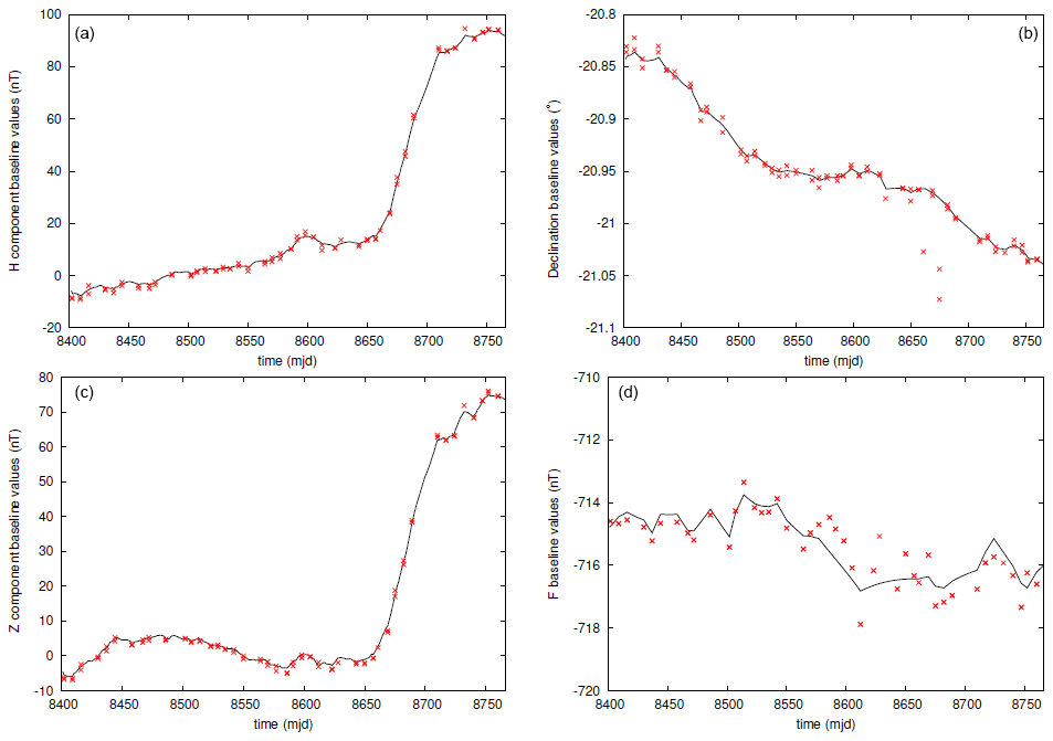
Figure 6 Estimated baseline values of La Réunion observatory, presented in a HDZF format, for the year 2023. The time unit is “modified Julian day” (mjd) – i.e. decimal day number starting from 1 January 2000 at 00:00 UT. The values derived from absolute observations are shown in red and the estimated daily values in black.

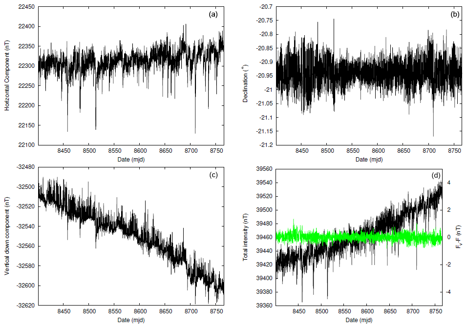
Figure 7 Estimated calibrated hourly mean magnetic data at La Réunion observatory. The date unit is “modified Julian day” (mjd) – i.e. decimal day number starting from 1 January 2000 at 00:00 UT. The data are presented in a HDZF format, for the whole year 2023. The ΔF values derived from the hourly means of the vector and scalar values are shown in green. The corresponding scale is shown on the right side of the plot.

3.3 Calibrated data for year 2023

Calibrated data, estimated from the variation vector data using the baseline values of Fig. 6, are presented in Fig. 7. The horizontal component presents the expected large-amplitude fast variations that are associated with perturbations of the ionosphere–magnetosphere system by the sun activity. There is nonetheless a small trend of increasing intensity by roughly 50 nT over 2023. The trend is even stronger on the vertical component that increases by around 100 nT in absolute value in the year. The combined effect of these variations produces an increase in the magnetic field strength approximately from 39 420 to 39 530 nT – i.e. an annual variation of the order of 100 nT yr⁻¹ that corresponds roughly to what was predicted by the International Geomagnetic Reference Field (IGRF) version 13 (Alken et al., 2021): 104 nT yr⁻¹ in 2023. For this same IGRF, and the same location as the observatory, the expected variation in the vertical component is largely underestimated, and so is the expected variation in declination. The values of the field components, as provided by the IGRF model, also differ significantly from the measured values. For 1 June 2023, the IGRF gives −19.515° in declination, 22 690 nT in the horizontal component, −31 458 nT in the vertical component, and 38 787 nT in total intensity. The observed differences are easily explained by the strong lithospheric signal generated by the surrounding volcanic rocks that is not accounted for in the IGRF.

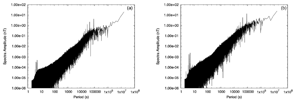
Figure 8 DFT amplitude spectra derived from time series of second data recorded in La Réunion magnetic observatory, from 1 July to 31 December 2023. (a) Spectrum derived from the vertical down component and (b) spectrum derived from the horizontal component.

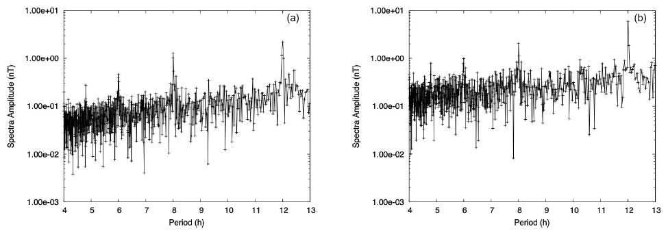
Figure 9 Zoomed-in view of the 4–13 h period range of the DFT amplitude spectra derived from second-resolution time series, recorded in la Réunion magnetic observatory, from 1 July to 31 December 2023. (a) Spectrum derived from the vertical down component and (b) spectrum derived from the horizontal component.

In the same figure (Fig. 7), the bottom-right plot also presents, in green, the calculated ΔF values for the year. The scale is given on the right side of the plot. Values vary well inside 1 nT around zero. This is a clear indication that the process applied to estimate the baseline values is a success.

As a final test to assess the quality of the observatory recorded signal, we computed the discrete Fourier transform (DFT) amplitude spectra of the vertical and horizontal components of the observed, de-trended, magnetic field variation second data over 6 months from July to December 2023 (see Fig. 8). Over this time interval, only five consecutive second-data records were missing. The gap has been filled by linear interpolation. Of course, as only variation data have been used, the time series have not been treated to remove possible anthropological noise, and furthermore the longest periods of the spectra are not reliable as the baseline correction has not been applied. Strong peaks are obvious at periods of 24, 12, 8, 6, 4.8, and 4 h (see also Fig. 9 for a zoomed-in view of periods ranging from 4 to 13 h). These periods correspond to the S1–S6 solar diurnal tidal constituents (see, for example, Love and Rigler, 2014, regarding tidal signals in observatory data). However, in magnetic data these peaks mainly result from the rotation of the Earth inside the magnetosphere combined with the signal associated with the S_q current system in the ionosphere. There are no other clear tidal periods peaking out of the spectra, except possibly at 12.42 h for the M2 (lunar semi-diurnal) tide in Fig. 9a. However, this period does not correspond to a peak in the horizontal component spectra. There are few peaks in the lowest periods of Fig. 8, in particular for a period of 5 s. This is clearly due to cross-talk of the scalar/vector electronics as 5 s is our sampling period for scalar variometer data. At even shorter periods, the spectra collapse due to the filtering of the lowest periods applied to second data, as recommended in intermagnet (2020). Overall, this Fourier analysis does not reveal major difficulties in the observatory data. There is a relatively low level of anthropological noise at the La Réunion observatory site.

4 Conclusions

We presented the setting and location of the La Réunion Island observatory and the data processing algorithms applied to compensate for the effects of the large magnetic gradients typical for volcanic islands. This observatory has been established to fill a geographical gap in the Indian Ocean part of the global observatory network. Calibrated data have been estimated for the full year of 2023.

Similar to other observatories situated on a volcanic island, the magnetic field induced by local geology is significant and exhibits steep gradients. We have shown that one of the effects of these gradients is a variation during a single day of the differences of field strength between two sites only a few metres apart. To reconcile the magnetic field strength observed by the variation vector magnetometer with the magnetic field strength measured by the variation scalar magnetometer, one simply has to estimate the large local contribution of the magnetized rocks to the observed vector magnetic field. These estimates do not have to be very accurate, and in the case of La Réunion observatory they are of −2400, 280, and −20 nT in the X, Y, and Z vector component, respectively, in the sensor reference frame.

The obtained calibration parameters – i.e. the “baseline values”, show a strong drift within the year 2023, particularly during the month of October. This is very likely due to the fact that pillars have been built only recently on the observatory site and are still settling. We therefore expect the baseline values to stabilize and present only minor drifts in the years to come. For 2023, we are however confident that the calibrated observatory vector data are reasonably accurate as the drift of the δF values remains weak, and the fit to the absolute observation is good.

The iaga code given to this observatory is reu.

Appendix A: Derivation of Eq. (4)

The total intensity on the variometer pillar is

$$\begin{array}{}\text{(A1)}& F_{\mathrm{v}}=\sqrt{x_{\mathrm{v}}^{\mathrm{2}}+y_{\mathrm{v}}^{\mathrm{2}}+z_{\mathrm{v}}^{\mathrm{2}}},\end{array}$$

whereas on the observatory main pillar it is

$$\begin{array}{}\text{(A2)}& F_{\mathrm{p}}=\sqrt{(x_{\mathrm{v}}+\mathit{\delta }x{)}^{\mathrm{2}}+(y_{\mathrm{v}}+\mathit{\delta }y{)}^{\mathrm{2}}+(z_{\mathrm{v}}+\mathit{\delta }z{)}^{\mathrm{2}}}.\end{array}$$

The latter quantity can be approximated by

$$\begin{array}{}\text{(A3)}& F_{\mathrm{p}}\simeq \sqrt{x_{\mathrm{v}}^{\mathrm{2}}+y_{\mathrm{v}}^{\mathrm{2}}+z_{\mathrm{v}}^{\mathrm{2}}+\mathrm{2}(x_{\mathrm{v}}\mathit{\delta }x+y_{\mathrm{v}}\mathit{\delta }y+z_{\mathrm{v}}\mathit{\delta }z)},\end{array}$$

where terms in second order of δx, δy, or δz are neglected. It follows that

$$\begin{array}{}\text{(A4)}& F_{\mathrm{p}}\simeq F_{\mathrm{v}}\sqrt{\mathrm{1}+\mathrm{2}(x_{\mathrm{v}}\mathit{\delta }x+y_{\mathrm{v}}\mathit{\delta }y+z_{\mathrm{v}}\mathit{\delta }z)/(x_{\mathrm{v}}^{\mathrm{2}}+y_{\mathrm{v}}^{\mathrm{2}}+z_{\mathrm{v}}^{\mathrm{2}})},\end{array}$$

or alternatively

$$\begin{array}{}\text{(A5)}& F_{\mathrm{p}}\simeq F_{\mathrm{v}}[\mathrm{1}+(x_{\mathrm{v}}\mathit{\delta }x+y_{\mathrm{v}}\mathit{\delta }y+z_{\mathrm{v}}\mathit{\delta }z)/F_{\mathrm{v}}^{\mathrm{2}}],\end{array}$$

where the quantity $(x_{\mathrm{v}}\mathit{\delta }x+y_{\mathrm{v}}\mathit{\delta }y+z_{\mathrm{v}}\mathit{\delta }z)/F_{\mathrm{v}}^{\mathrm{2}}$ is assumed to be small. Here again, higher-order terms are neglected. The difference F_p−F_v is therefore

$$\begin{array}{}\text{(A6)}& F_{\mathrm{p}}-F_{\mathrm{v}}\simeq (x_{\mathrm{v}}\mathit{\delta }x+y_{\mathrm{v}}\mathit{\delta }y+z_{\mathrm{v}}\mathit{\delta }z)/F_{\mathrm{v}},\end{array}$$

and noticing that the right-hand side of Eq. (A6) is the result of a vector scalar product, Eq. (4) follows. The same result can be obtained by simply using a first-order Taylor series for the total field intensity at the main observatory pillar:

$$\begin{array}{}\text{(A7)}& F_{\mathrm{p}}\simeq F_{\mathrm{v}}+{\displaystyle \frac{\partial F_{\mathrm{v}}}{\partial x_{\mathrm{v}}}}\mathit{\delta }x+{\displaystyle \frac{\partial F_{\mathrm{v}}}{\partial y_{\mathrm{v}}}}\mathit{\delta }y+{\displaystyle \frac{\partial F_{\mathrm{v}}}{\partial z_{\mathrm{v}}}}\mathit{\delta }z.\end{array}$$