Frequency control and monitoring of the ALOMAR RMR lidar's pulsed high-power Nd:YAG lasers

Doppler wind measurements in the middle atmosphere by ground-based lidar are challenging and benefit from precise spectral characterization of the laser source. We present a system for frequency control and monitoring of pulsed commercial high-power Nd:YAG lasers, which is entirely software controlled, automated, and works in real-time. It basically consists of an embedded controller handling the cavity control of the injection-seeded power laser and an embedded controller based spectrometer performing the spectral analysis of each individual power laser pulse using a Fabry-Pérot etalon. The power laser cavity length is optimized by pulse build-up time minimization, yielding a stable long-term single-mode operation. The spectrometer is able to analyze continuous-wave as well as pulsed lasers with repetition rates of 100 Hz and resolves frequency changes of less than 300 kHz, corresponding to a resolution of ∼ 5 × 10⁻¹⁰ at a wavelength of 532 nm.

1 Introduction

Active remote sensing of the Earth's atmosphere using optical methods was already proposed more than 130 years ago (Jesse, 1887). Shooting a “bundle of intensive collimated electric light” should be used to determine the altitude of clouds in the mesopause region from 80 and 90 km altitude, the so-called noctilucent clouds. It took more than 60 years for this method to be applied successfully for the first time. A system of two searchlight mirrors as the transmitter and receiver optics, a high-voltage spark between aluminum electrodes as a light source, and a photoelectrical cell as a detector was used to measure cloud-base heights up to 5.5 km in daylight (Jones, 1949). The invention of the laser (light amplification by stimulated emission of radiation) in 1960 (Maiman, 1960) opened up new opportunities for active optical remote sensing with lidar (light detection and ranging) instruments. At present, lidars are commonly used to investigate the atmosphere by determining parameters like, e.g., temperature, winds, aerosols, densities of atmospheric constituents and trace gases, and cloud altitudes.

The Leibniz Institute of Atmospheric Physics operates a powerful Rayleigh/Mie/Raman (RMR) lidar in the Arctic Lidar Observatory for Middle Atmosphere Research (ALOMAR) in Northern Norway (69° N, 16° E). This twin-lidar went into operation in 1994 and its technical performance was continuously improved since then (Fiedler and Baumgarten, 2024). It was designed from the outset for multi-parameter investigations of the Arctic middle atmosphere on a climatological basis. In 2008, the lidar was upgraded to a direct detection Doppler lidar by the integration of the Doppler Rayleigh Iodine Spectrometer (DORIS) (Baumgarten, 2010). The ALOMAR RMR lidar is one of the longest operating middle atmosphere lidars and the only one measuring aerosols, temperature, and horizontal winds simultaneously and during day and night.

Wind measurements by the ALOMAR RMR lidar are based on measuring the Doppler shift of laser photons scattered back on air molecules. The Doppler shift for 1 m s⁻¹ wind speed is approx. 4 MHz (Δλ∼4 fm) at a wavelength λ of 532 nm, corresponding to $\mathrm{\Delta }\mathit{\lambda }/\mathit{\lambda }\sim {\mathrm{10}}^{-\mathrm{8}}$. Such measurements are challenging in the middle atmosphere due to the exponentially decreasing air density with height. The lidar uses two sets of power lasers (∼ 1 J pulse energy at 1064 nm and 100 Hz repetition rate) and steerable receiving telescopes (1.8 m diameter primary mirror) for highest possible signal in two simultaneous viewing directions. For a detailed description of the lidar the reader is referred to Fiedler and Baumgarten (2024). To operate both lidar transmitters precisely at the same wavelength, the power lasers are injection-seeded using a single external seed laser. The seed laser acts as an optical frequency standard for the lidar as its light is also used in the lidar receiver. However, the seeding method as well as the seeding process itself create frequency deviations of the generated power laser pulses with respect to the seeder, which are relevant for the Doppler shift determination of the received light from the atmosphere.

There are mainly two approaches to quantify these deviations, optical heterodyne detection against a frequency-stable laser source and spectral analysis of the laser output using interferometers (Fabry-Pérot and Fizeau). Heterodyne measurements with different pulsed laser setups have shown standard deviations for the frequency stability down to ∼ 2 MHz (e.g., White et al., 2004; Schröder et al., 2007; Xia et al., 2012; Wang et al., 2020). State-of-the-art commercial wavelength meters achieve similar values. Spectrometer based solutions reach frequency resolutions down to 10⁻⁷ (e.g., Morris et al., 1984; Koo and Akamatsu, 1991; Faust and Klynning, 1991; Hahn et al., 1993). Because existing systems did not meet our requirements we have developed our own solution as a robust Fabry-Pérot based spectrometer which determines the frequency stability of a power laser for each single laser pulse in real-time. In the following sections we report on the frequency control of the ALOMAR RMR lidar power lasers (Sect. 3) as well as the laser pulse spectrometer (Sect. 4) and give examples of its sensitivity and performance (Sect. 5).

2 System setup

Figure 1 shows the block diagram of the “Frequency Control and Monitoring” (FCaM) system for one power laser. The schematic contains only key components of the system.

Figure 1 Schematic of the “Frequency Control and Monitoring” (FCaM) system for one power laser. M: mirror on piezo phase shifter, PC: Pockels cell, P: polarizer, M%: output mirror, PD: photodiode, SHG: second harmonic crystal, L: lenses, BS: beam splitter cube, D: diffuser, red and green lines: 1064 and 532 nm laser light.

The upper part of the diagram refers to the control of the power laser frequency. The seeder is a continuous-wave (CW) single-mode Nd:YAG laser (Innolight Prometheus-100NE) generating both the fundamental and second harmonic wavelengths, which are phase-locked to each other. The laser provides frequency tuning, both slow over a larger range via the laser crystal temperature and fast over a narrow range via a piezo element on the laser crystal. Both tuning parameters can be controlled with external voltages applied to the laser head and are used for an absolute frequency stabilization of the seed laser output to a steep slope of iodine absorption line 1109 (λ_vac∼532.260 nm) by absorption spectroscopy with a long-term stability better than $\mathrm{\Delta }\mathit{\lambda }/\mathit{\lambda }={\mathrm{10}}^{-\mathrm{8}}$ (Fiedler and Baumgarten, 2024).

Seeder radiation at 1064 nm is coupled into the power laser for injection seeding to obtain pulses of high power with a narrow linewidth. The power laser is a pulsed diode-pumped Nd:YAG laser (Innolas EVO-IV) operating at 100 Hz repetition rate and consisting of a two-stage oscillator, a two-stage amplifier, and nonlinear crystals for frequency doubling and tripling. Both the pump diodes and the Pockels cell are triggered externally as components of the lidar trigger system. A fast photodiode generates the timing signal of the outgoing power laser pulse, which is used for the seeding control. Part of the frequency doubled radiation is used for spectral analysis.

The lower part of Fig. 1 refers to the laser pulse spectrometer used for monitoring the frequency deviations between power and seed laser. The CW seed laser light at 532 nm is chopped by a mechanical chopper and coupled, together with power laser light, into an etalon via a beam splitter cube. A camera detects the interference ring patterns of light from both lasers.

The entire system is operated by two real-time controllers, which, among other things, handle the trigger and seeding process and analyze the frequency stability of the power laser pulses. The system will be described in detail in the following sections.

3 Pulsed Nd:YAG laser frequency control

The power laser uses injection seeding in combination with active Q(quality)-switching by a Pockels cell inside the optical resonator (the path between M and M% in Fig. 1). Light from the seed laser is coupled into the resonator to seed it with the desired wavelength. To ensure that the frequency of the power laser pulse matches that of the seed laser closely, the resonance frequency of the power laser oscillator needs to be controlled. We use the standard method (Rahn, 1985), called “pulse build-up time reduction”, which is often used in commercial Nd:YAG lasers with build-in seeder. For high-quality cavity control, we have developed a custom software based system. The highly reflecting mirror M is mounted on a piezo phase shifter (Physik Instrumente S-303) with a 3 µm travel range and is driven by a piezo amplifier module (Physik Instrumente E-831). This setup allows the piezo position to be set by an embedded controller analog output voltage, enabling control of the power laser oscillator length with sub-nanometer resolution. The time delay between opening of the Q-switch and the laser pulse leaving the oscillator is termed the pulse build-up time (BuT). When the Q-switch is operated only one round trip of seed laser radiation will be present in the oscillator which is spectrally broadened due to the Q-switch. So the adjacent longitudinal modes will always receive a higher start energy than other longitudinal modes. As the oscillator mode is better matched to the seed laser wavelength and mode, other modes get suppressed more until the gain of the laser is used up. This emission is orders of magnitude stronger than the spontaneous emission from the laser medium. Therefore, a Q-switched pulse will build up sooner out of the seeded emission compared to spontaneous emission. The shorter the BuT value the better seed and power laser frequencies match. Hence, the BuT value serves as a measure for the quality of the seeding process. For the BuT measurement, the Q-switch trigger signal and the output from a fast photodiode looking at leakage light behind the laser cavity are used. The time difference of these two signals is determined by a time-to-digital converter chip (ScioSense TDC-GP22) with a resolution of ∼ 90 ps.

Control of the power laser cavity length as well as the BuT measurement are performed by an embedded controller (National Instruments sbRIO-9637). This controller is a single-board device and contains a field-programmable gate array (FPGA), reconfigurable input–output hardware, and runs a real-time operating system (RT-Linux). Both the RT application software and the FPGA are programmed with the graphical programming system LabVIEW. The software design is based on a client / server architecture that allows the controller to act as a stand-alone device (server). The user interface software (client) is not necessary for the operation but can run on any computer in the network for visualization of ongoing processes and parameter changes. The embedded controller is integrated into a 19 in. enclosure, together with additional electronics for trigger $I/O$ and signal conditioning (laser controller). In order to generate the error signal for the BuT minimization, the voltage controlling the cavity length is modulated with a small-amplitude sinusoidal signal with a period of ∼ 30 power laser pulses. Then the minimum BuT value is determined over one cycle and the corresponding voltage for the piezo phase shifter is set. Near the lower and upper limits of the piezo displacement range a voltage jump is initiated to reset the piezo to an approximately center position.

Figure 2 shows the behavior of the cavity control during the first 2 operation hours of the power laser after switch-on. In the beginning, the BuT values dropped quickly from 132 to ∼ 120 ns, which corresponds to the transition to stable seeding conditions. The warm-up phase of the laser takes approx. 2 h and impacts several laser parameters, such as e.g. the cavity length. This can easily be seen in changes in the voltage controlling the piezo position, which is mostly increasing between the reset points at the limits of the piezo displacement range. During the first hour shown in Fig. 2 seven position resets occurred, indicated by voltage jumps of 7.3 V, in order to keep the cavity length constant. This corresponds to a compensation of the thermal expansion of the laser structure by ∼ 11 µm. During the next hour, the warm-up process already slowed down and only two position resets of the piezo occurred. The BuT standard deviation from ∼ 703 700 measurements during the time period of 2 h is 0.6 ns.

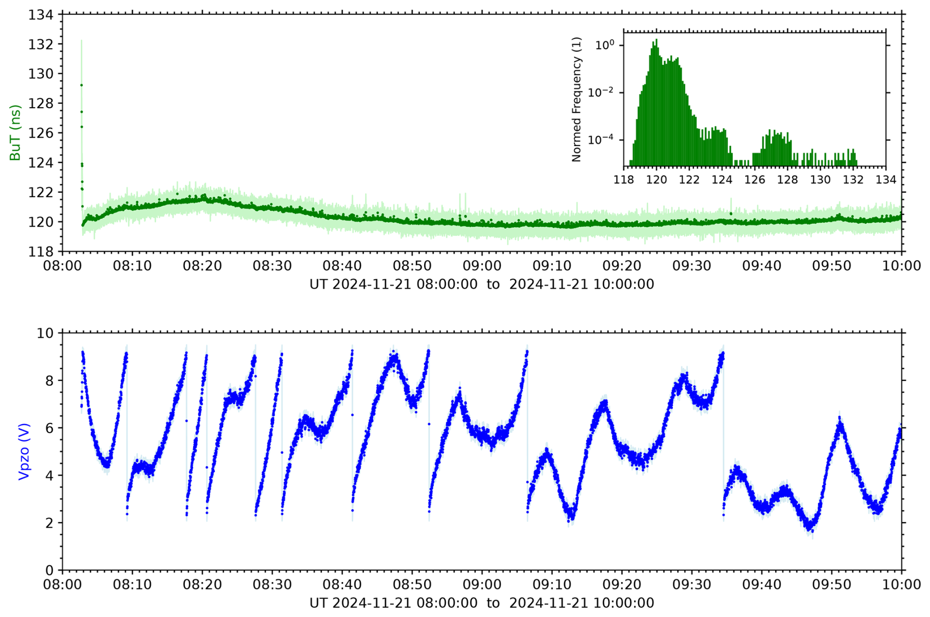
Figure 2 Nd:YAG laser cavity control during the first 2 operation hours after switch-on. Each single laser pulse was recorded, corresponding to a total of ∼ 703 700 datasets. The upper panel shows the build-up time (BuT, green) and the lower panel the piezo voltage controlling the cavity length (Vpzo, blue). The points are mean values over 1 s (100 laser pulses) and the light colors show minima and maxima during these periods. The histogram in the upper panel contains all individual values for the build-up time.

4 Laser pulse spectrometer

For monitoring the spectral stability of the power laser, we have developed a system which analyzes each individual laser pulse in real-time. This laser pulse spectrometer (LPS) uses light from the seed laser and the power laser and determines the frequency difference. The frequency difference, rather than the absolute frequency of the power laser, is of special interest for the analysis of power laser light scattered in the atmosphere, because for measuring the Doppler shift a similar iodine absorption spectroscopy setup is used as for the seed laser stabilization. The LPS is based on an air-spaced Fabry-Pérot etalon having 1 GHz free spectral range, a clear aperture of 35 mm, a mirror reflectivity of 93 %, and a finesse > 25 (LightMachinery, Inc). The free spectral range value was chosen to achieve high spectral resolution in the area of Doppler broadened iodine lines. The etalon converts spectral information of the laser light into two-dimensional spatial information represented by interference fringes.

A small portion of the main power laser beam (∼ 0.5 %) containing all three wavelengths is split off by an anti-reflection coated wedge plate. A dichroic mirror separates the 532 nm light and directs it to the beam splitter cube of the LPS. Seed laser light at 532 nm is guided via single-mode optical fiber to the LPS and enters the beam splitter cube after modulation by a rotating chopper. For a minimum beam diameter in the plane of the chopper blade the seed laser light passes a bi-convex lens (40 mm focal length) after leaving the optical fiber. The beam splitter cube combines both beams into a single output beam having a diameter of ∼ 15–20 mm at the entrance of the etalon. There the angular distribution of the light is increased by a ground glass diffuser (1500 Grit) before the light enters the etalon. The angular interference pattern produced by the etalon is transformed into a spacial interference ring pattern on the camera chip using a lens with 500 mm focal length. The camera is a USB3-camera having 1.3 M pixel at 7.9 mm sensor diagonal (Basler acA1300-200um). To speed up data processing the camera chip resolution is halved by binning 2 pixels in each direction.

A special trigger scheme is required for the LPS to work with a CW and a pulsed laser. Light from the CW seed laser is chopped in such a way that it enters the etalon between two power laser pulses by synchronizing the rotating chopper to the 100 Hz trigger pulses for the power laser. The camera is triggered to read out every power laser pulse and seed laser light from one intra-pulse period every second (defined by the exposure time). Trigger pulse handling, image acquisition and data processing are done by an industrial controller (National Instruments IC-3173). Like the device for the laser frequency control, the LPS controller contains a FPGA, reconfigurable input–output hardware, runs RT-Linux, and is programmed using LabVIEW. Again, the software is designed following a client / server architecture and the LPS controller works as stand-alone device. After acquisition of a camera image, the positions of individual interference ring pattern are determined and the total intensity of each ring in radial direction is calculated by integration over camera pixel with the same radial distance. This yields a 1-dimensional relationship of intensity as function of radius in pixel coordinates. Then, for each peak of this function the position and amplitude of the maximum as well as the full width at half maximum (FWHM) are calculated. The determination of these parameters does not involve fitting of functions, which might fail in case of weak light intensities. In order to obtain fractional pixel resolution we use the following processing chain:

• Determination of peak maxima and background level in the 1 d array of intensity as function of radius in pixel coordinates.

• Tracking the intensity values from a peak maximum in left and right direction until the background level is reached yield arrays for the left and right slopes of the peak.

• For each slope array: finding the two intensity values between which the half maximum value of the peak lies.

• Linear interpolation of the half maximum value using fractional pixel values yield left and right positions of the FWHM value. The difference between these positions yields the FWHM value in fractional pixels.

• The sum of the left position of the FWHM value and the half of the FWHM value yields the position of the peak maximum in fractional pixels.

Figure 3 shows camera images and intensities as function of radius displayed in the user interface of the LPS client for one seed and one power laser data acquisition.

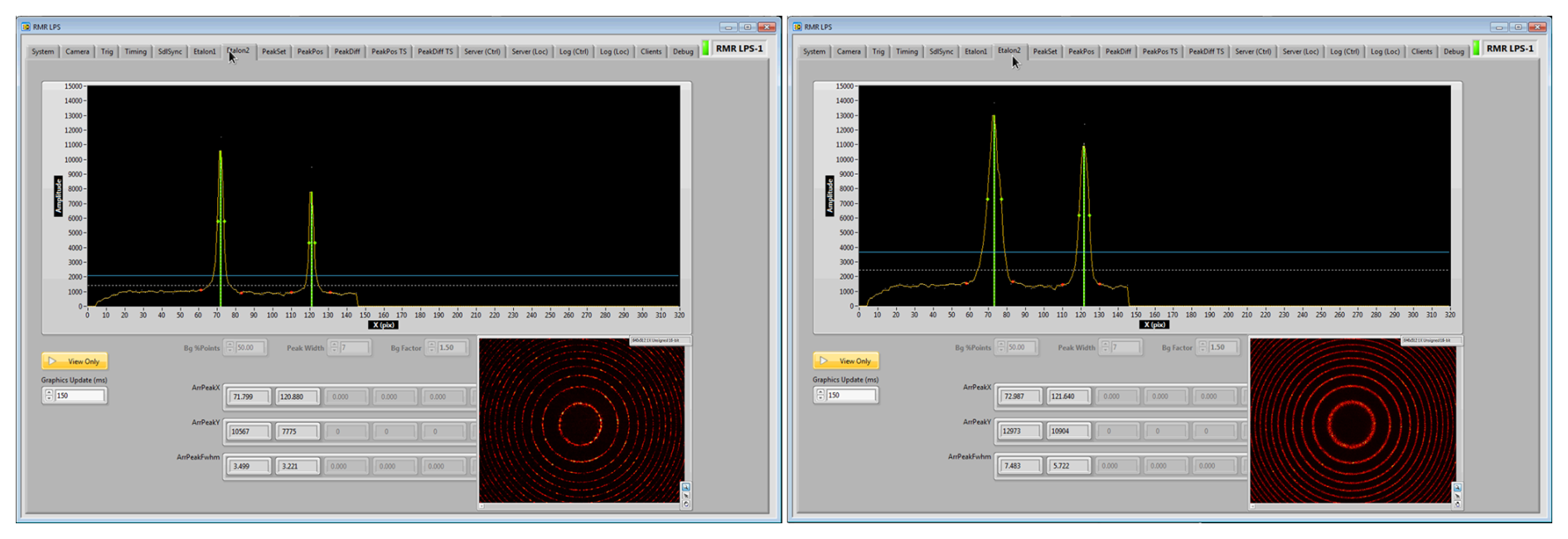
Figure 3 Screenshots of the LPS client user interface. The left panel shows data from one image with seed laser light, the right panel the same for one power laser pulse. Red circles are interference ring patterns as detected by the camera. Peak parameters are calculated from cross sections of the inner two rings. For details see text.

The pixel difference in the peak positions of seed and power laser light is a measure for their frequency difference. Such pixel differences are calculated for each power laser pulse acquired in 1 s with respect to the seed laser light acquired in the previous second. This procedure eliminates the impact of changes in etalon parameters caused by drifts in temperature and air pressure that generally occur on much larger timescales. Finally, the pixel values are converted to frequencies.

To ensure that all data processing is finished before the acquisition of the next image the software is highly parallelized. This is supported by the programming language, which makes it relatively easy to program multiple tasks that are performed in parallel via multithreading. Additionally the code on the RT level was structured in a way that more complex calculations are separated from time-critical parts of the code and the data transfer between them is done by FIFO (first-in, first-out) structures. To further improve the timing, user interaction and file operations (writing logs etc.) are outsourced to the client on a computer running Microsoft Windows, which communicates with the server (embedded controller) via network shared variables.

4.1 Calibration

In the setup for the stabilization of the seed laser, 532 nm radiation is guided through an iodine vapor cell and the light intensity is determined before and behind the cell (Fiedler and Baumgarten, 2024). The ratio of these intensities (behind / before) is a measure of the absorption. The LPS was calibrated by tuning the wavelength of the seed laser over a part of the iodine absorption spectrum around line 1109. During this procedure the position changes of the inner two peaks of the interference ring patterns were followed. At the same time the absolute wavelength of the seed laser was monitored using a commercial wavelength meter Ångstrom WSU-30 (HighFinesse GmbH) having an accuracy of 30 MHz. The scan covered ∼ 6 GHz as indicated by the wavelength meter, corresponding to approx. six free spectral ranges of the etalon as indicated by the interference patterns acquired by the LPS. During each cycle, corresponding to one free spectral range, the innermost peak moved roughly from pixel position 20 to 100 and the adjacent peak from pixel position 100 to 135 on the camera. Data from all six cycles were merged to obtain a mean relationship between camera pixel position and relative frequency. The result is the continuous mapping of ring radii to relative frequency, with the range in pixel position 20 to 135 corresponding to a change in frequency of ∼ 1.8 GHz.

The mapping of pixel coordinates to frequency is shown in Fig. 4. The upper panel shows the measured data from all cycles and a 4th degree polynomial fit. From the fit the frequency slope, representing the frequency change from one camera pixel to the next, is calculated and shown in the lower panel. These values are used by the LPS controller to convert pixel to frequency deviations. The linear relationship between frequency slope and location change of the interference pattern on the camera is almost perfect.

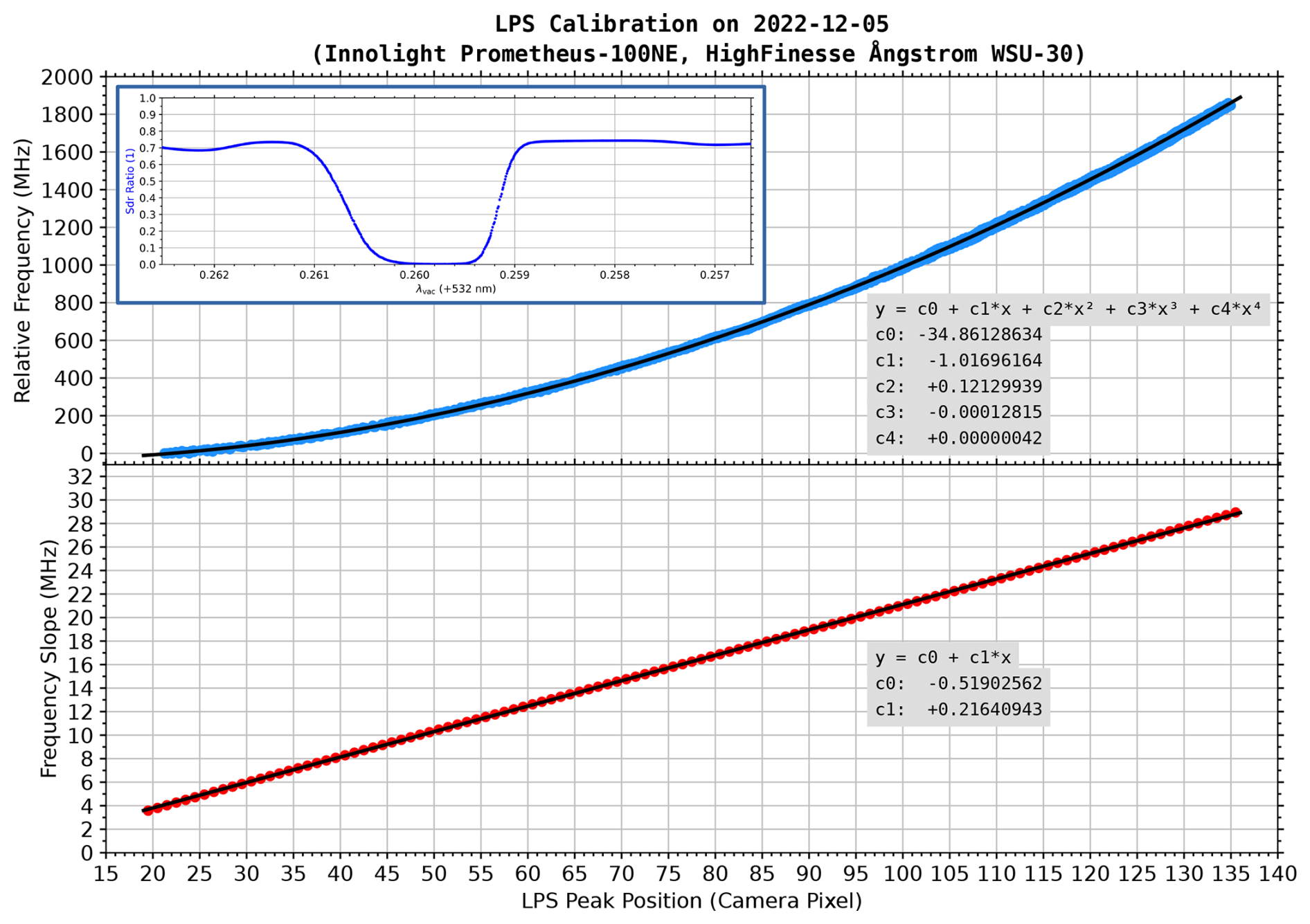
Figure 4 Calibration of the laser pulse spectrometer using the seed laser and a wavelength meter. The frequency scan of the seed laser took 14 min, corresponding to ∼ 6 GHz frequency change, and covered the entire iodine absorption line 1109. Upper panel: measured (blue circles) and fitted (black line) relative frequency as function of interference ring position on the camera. Lower panel: slope for each camera pixel from the fit in the upper panel, representing the frequency change from one pixel to the next (red circles). The linear regression line is shown in black. The small insert in the upper panel shows the simultaneously measured iodine absorption using the iodine vapor cell of the optical setup for the seed laser frequency stabilization.

4.2 Sensitivity

To estimate the accuracy and resolution of the LPS, we used the seed laser with the same optical setup as for the calibration measurement, but now having the seed laser frequency locked to a target ratio value of 0.6 on the increasing slope of iodine absorption line 1109 at λ_vac∼532.25903 nm (see absorption spectrum shown in Fig. 4). Deviations from the target ratio are caused by frequency changes of the seed laser. For the LPS sensitivity tests the rotating chopper, which usually synchronizes the seed and power laser light to each other, is not operated and seed laser light enters the LPS continuously. The camera is operated with the usual 100 Hz trigger for the power laser, resulting in 100 spectral measurements of the seed laser light per second.

Figure 5 shows a 5 s time series of the seed laser light intensity ratio measured with the iodine vapor cell and the peak position from the inner interference ring at the camera. The single values were additionally smoothed using a Savitzky-Golay filter (window length: 11, order: 3). It is obvious that both smoothed curves show similar variations for most of the time, which means that the LPS even detects the very small frequency fluctuations while the seed laser is stabilized. The fluctuations shown here cause only sub-pixel changes of the interference pattern on the camera, corresponding to frequency changes well below 1 MHz. To quantify the LPS sensitivity, we calculated the correlation of both time series on the basis of linear regression analysis, resulting in Pearson correlation coefficients of 0.62 (0.82) for single (smoothed) values. In a next step we investigated a total time period of 12 h, containing 8640 consecutive 5 s periods with 500 measurements each. The lower panels of Fig. 5 show the correlation coefficients as function of peak position ranges for each period. The peak position range is defined as the maximum value minus the minimum value found within each period of time. The plots solely contain data for positive and significant correlations (r > 0, p value < 5 %). These limits were violated by 11 % (6 %) of the single (smoothed) values. The small number of data points with violated selection criteria (∼ 10 % at 300 kHz range) demonstrates that the LPS can measure frequency changes down to ∼ 300 kHz with a success rate of 90 % or better, corresponding to $\mathrm{\Delta }\mathit{\lambda }/\mathit{\lambda }$ ∼ 5 × 10⁻¹⁰. For smoothed values the resolution improves to ∼ 150 kHz.

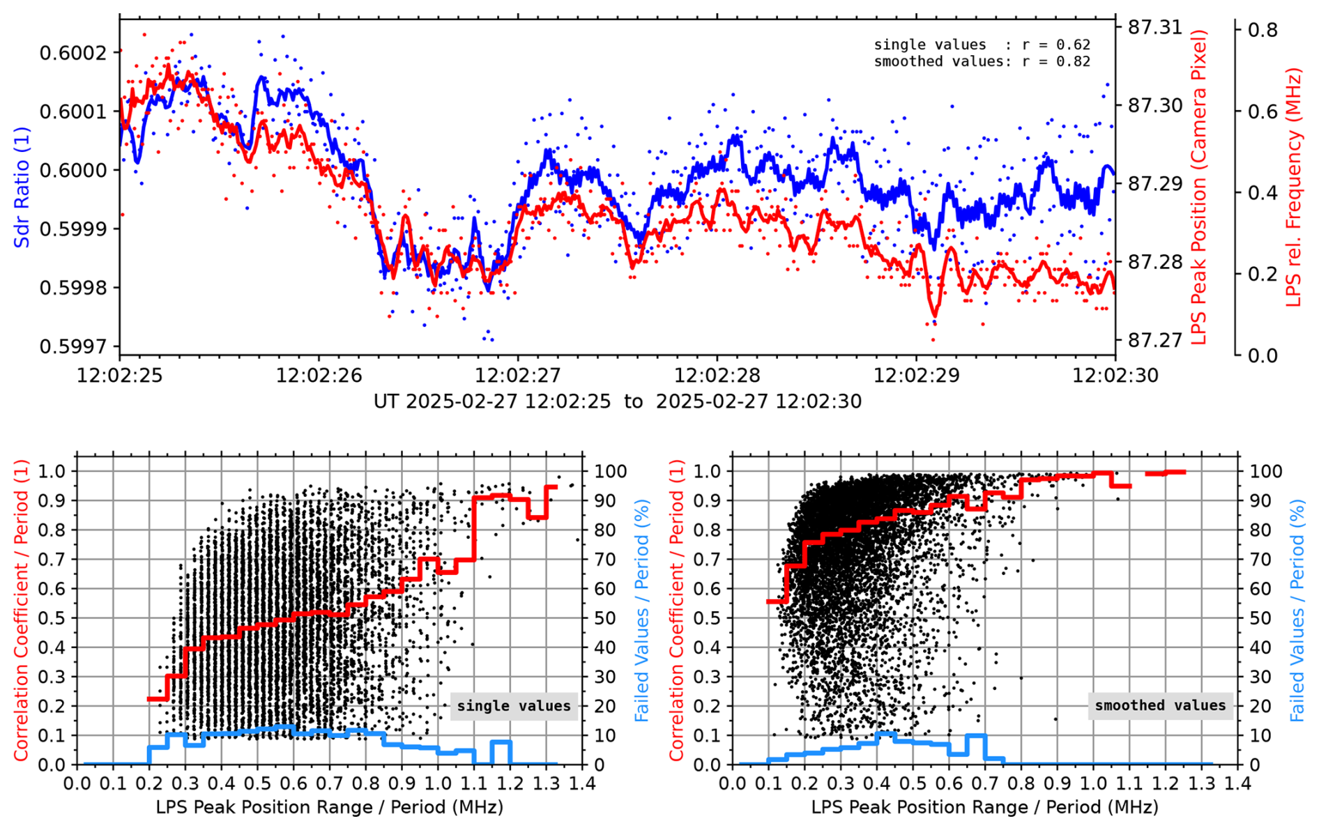
Figure 5 Upper panel: frequency fluctuations of the stabilized seed laser during a 5 s time period quantified as changes in laser light intensity ratio at the iodine vapor cell (Sdr Ratio, blue) and the position of the inner interference ring at the LPS camera (LPS Peak Position, red). Camera pixels are converted to frequencies using the LPS calibration data. Single values (points) and smoothed values (lines) as well as Pearson correlation coefficients for both time series are shown. Lower panels: LPS sensitivity in terms of successful correlations between “Sdr Ratio” and “LPS Peak Position” for single (left) and smoothed (right) values during a total time period of 12 h (8640 single periods). Red step plots show median values of the correlation coefficient distributions per 50 kHz LPS peak position range. Blue step plots show percentage of failed correlations. For details see text.

5 FCaM Performance

Figure 6 shows the behavior of the power laser frequency control and monitoring during an atmospheric measurement as time series over 7 s. The BuT reduction method for the laser cavity control requires a modulation of the cavity length, which is done here by sinusoidal modulation of the piezo phase shifter holding the highly reflecting mirror with an amplitude of ±140 mV, corresponding to ±30 nm displacement of the mirror. After each cycle the DC component of the voltage is updated, causing jumps in the time series for Vpzo. The individual BuT measurements show a certain spread, a running mean with a length of 11 values reproduces the Vpzo variations. Periods with smaller responses to the mirror displacements possibly indicate electronic interference during the measurement process. The individual measurements of the power laser frequency stability reproduce the sinusoidal variation of the cavity length nearly perfectly. The voltage amplitude for cavity length modulation corresponds to approx. ±10 MHz variation of frequency deviation between power and seed lasers. These amplitudes could be further reduced as long as the stability of the BuT measurement is guaranteed. It would also be possible to use the measured frequency deviation by the LPS for the cavity control, as was done in Schaefer et al. (2019), but this is out of the scope of the current publication.

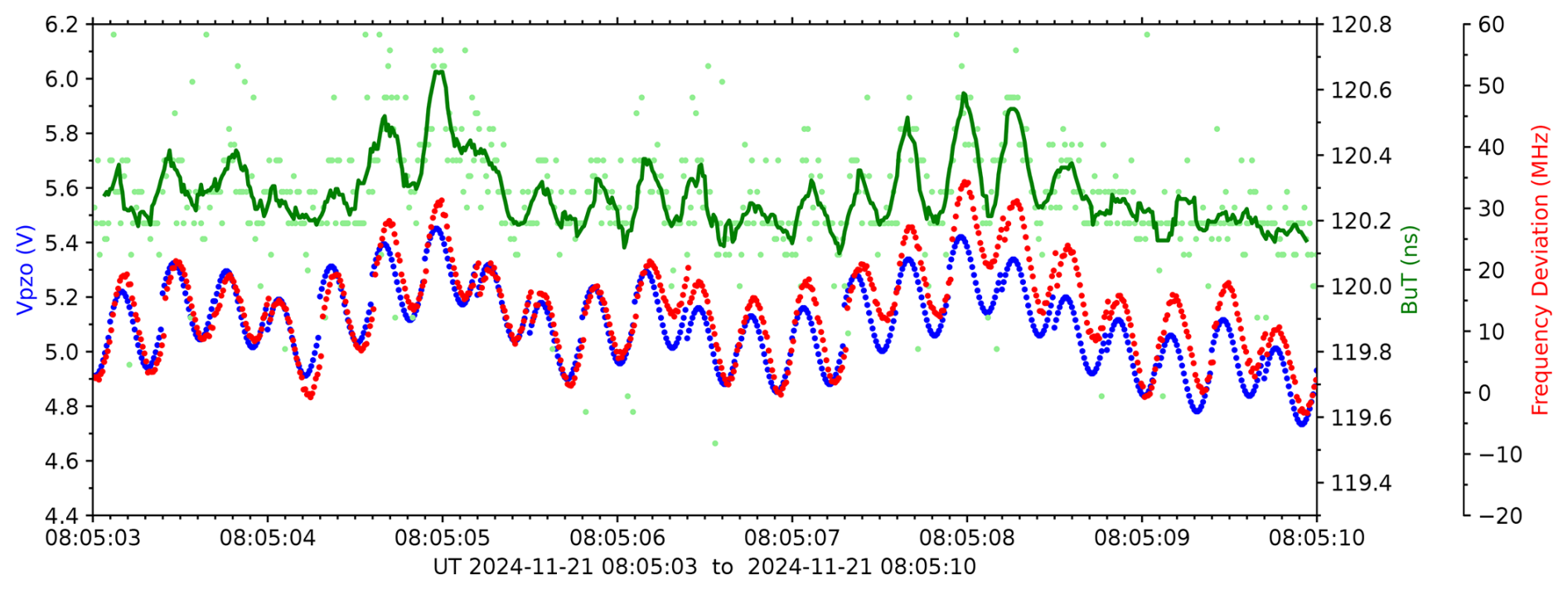
Figure 6 FCaM performance during a time period of 7 s (700 measurements for each parameter): piezo voltage controlling the cavity length (Vpzo, blue), build-up time (BuT, green), and frequency deviation between power and seed lasers (red). Single values are drawn as points, the running mean as line.

Figure 7 shows the frequency stability of seed and power laser during the same measurement in a time period of 10 min. The values refer to a period of 1 s, as the deviations for each laser are determined relative to the seed laser measurement from the previous second. The mean frequency deviation of the power laser is −1.74 MHz with a standard error of 44 kHz, the standard deviation of 10.76 MHz corresponds approx. to the cavity length modulation. As expected, the values are much smaller for the seed laser (standard error: 11 kHz, standard deviation: 273 kHz).

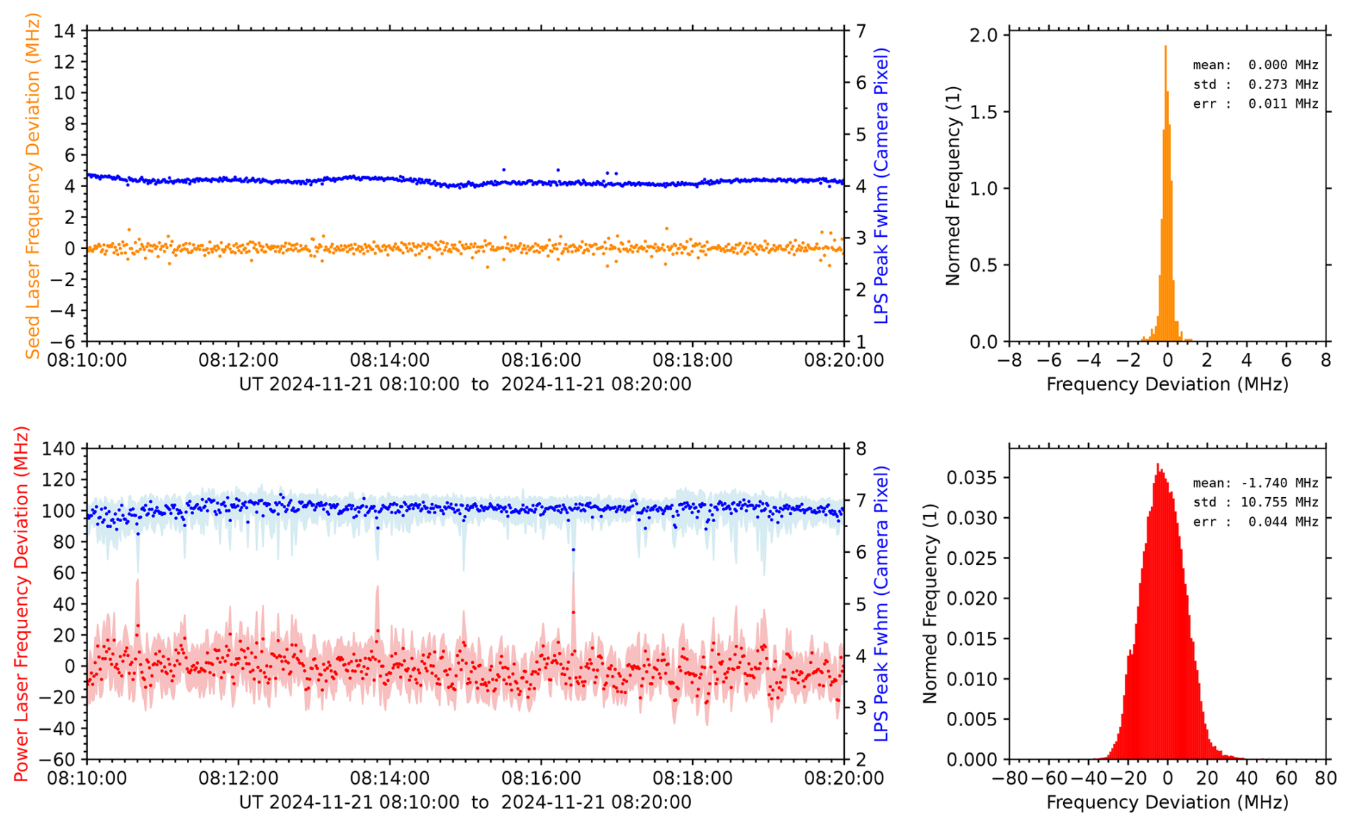
Figure 7 Frequency stability of the lasers during a time period of 10 min, corresponding to 600 seed laser (upper panels, orange) and 60 000 power laser (lower panels, red) measurements. The points are mean values over 1 s, minima and maxima during these periods are shown in light color. The histograms contain all individual values for the frequency deviations and the corresponding statistical mean, standard deviation, and standard error. The full widths at half maximum of the interference ring patterns on the camera are also shown in blue (Peak Fwhm). Please note that the axis scalings for power and seed laser frequency deviations differ by one order of magnitude.

The LPS software also determines the width of the interference ring patterns. Although the device is not designed to measure the linewidth of the laser, the peak parameters can give additional information about the performance of the power laser. We find larger values for the power laser frequency deviations to be accompanied by reduced peak widths. A closer look to the event around 08:16:45 UT suggests that the control loop did not follow the internal parameter changes of the power laser cavity fast enough, which resulted in decreased peak widths and simultaneously decreased peak maxima by ∼ 6 %. The BuT increased by ∼ 1 ns during this event. Unseeded laser operation can be ruled out as a reason because the BuT reduction from unseeded to seeded operation is larger than 12 ns, cf. beginning of time series in Fig. 2. An abrupt change from one longitudinal mode to another (mode hopping) is also unlikely, as for the given cavity length L of ∼ 90 cm a longitudinal mode spacing Δν of ∼ 167 MHz can be expected ($\mathrm{\Delta }\mathit{\nu }=c/\mathrm{2}L$, with c as speed of light). Destructive interference of adjacent longitudinal modes (mode beating) could explain the observed reduced pulse intensity but should result into a spectral broadening instead of narrowing. In the end, it is unclear which process led to the observed behavior.

6 Summary

We have reported on a system called FCaM for frequency control and monitoring of pulsed commercial Nd:YAG power lasers. Three of these systems are in routine operation for several years now, two systems in the twin Doppler RMR lidar at ALOMAR and one system in the Doppler RMR lidar at Kühlungsborn (Gerding et al., 2024). The FCaM system is entirely software controlled, automated, and works in real-time. It is integrated into the corresponding lidar environment and delivers descriptive data for each single laser pulse to a MQTT (Message Queuing Telemetry Transport) server in the lidar network, where other instruments can access this information. The motivation for the development was to improve the retrieval of Doppler winds by taking the frequency stability of the lidar transmitter into account.

Multi-year experience shows a stable behavior of the cavity control, resulting in stable long-term single-mode operation of the power lasers. The imprinted cavity length modulation for the BuT minimization method results in approx. ±10 MHz frequency modulation around the mean frequency of the power laser, which potentially can be reduced. The quality of the cavity control can be further improved by optimizing the algorithm running on the embedded controller. For a given example, the standard error of the mean power laser frequency within 10 min was 44 kHz, which translates into a Doppler wind error of just ∼ 11 cm s⁻¹. This is more than adequate compared to typical middle atmosphere horizontal wind speeds in the range of few metres per second to 100 m s⁻¹.

For the investigation of the sensitivity of the laser pulse spectrometer we used the seed laser which is actively stabilized by iodine absorption spectroscopy. During a 12 h period, residual frequency variations of the seed laser were analyzed 100 times per second and frequency changes down to ∼ 300 kHz, corresponding to $\mathrm{\Delta }\mathit{\lambda }/\mathit{\lambda }$ ∼ 5 × 10⁻¹⁰, could be detected with a success rate better than 90 % when using each individual measurement value. Moderate smoothing of the measured data doubled the sensitivity. The remaining uncertainties in laser frequency translate to 8 and 4 cm s⁻¹ in Doppler wind speed for single and smoothed values, respectively, which is again more than adequate for the analysis of Doppler winds measured by RMR lidars in the middle atmosphere. The application of the LPS principle is not limited to RMR lidars but can also be used with other Doppler lidar systems such as resonance fluorescence lidars for wind and temperature measurements in the mesosphere and thermosphere, or with any other lidar systems which require precise knowledge of transmitted wavelengths.