Integrated electrical resistivity tomography and geological characterization of the upper San José de Aloburo landslide, Pimampiro, Imbabura

Landslides are a major hazard in mountainous regions of the Ecuadorian Andes. This study examines the upper and accessible sector of the complex San José de Aloburo landslide, Imbabura Province, by integrating electrical resistivity tomography (ERT) with surface geological observations, three stratigraphic columns, and local grain-size information. Four Wenner-array ERT profiles were acquired with a low-cost, non-commercial system and imaged to approximately 35–40 m depth. The inverted sections contain broad low-resistivity domains (approximately 4–45 Ω m) and higher-resistivity domains reaching approximately 297 Ω m. Because electrical resistivity is non-unique with respect to lithology, moisture, porosity, weathering, and pore-fluid properties, these domains are interpreted jointly with the geological observations rather than as direct indicators of saturation, cohesion, or a mechanically verified slip surface. Geoelectrical boundaries in Profiles 1, 2, and 4 are spatially consistent with potential instability-related boundaries in the upper landslide sector, but this interpretation remains indirect and lacks borehole or geotechnical confirmation at depth. The stratigraphic columns document alternating ash and pumice/lapilli units, whereas the quantitative sieve analysis available for sample ANG-TOP-B-01 provides only local sedimentological support and is not extrapolated to the entire landslide. The integrated dataset demonstrates the value of combining ERT and field geology in a volcaniclastic Andean setting while also defining the limitations imposed by survey coverage, inversion non-uniqueness, seasonal hydrological variability, and incomplete archival documentation of the custom instrumentation.

1 Introduction

Landslides are important agents of landscape evolution and a major geohazard in populated mountainous regions. In the Ecuadorian Andes, steep relief, seasonal rainfall, heterogeneous volcanic and volcaniclastic materials, irrigation, and land-use changes can combine to produce conditions favorable to slope instability (Highland and Bobrowsky, 2008; Huggett and Shuttleworth, 2022; García and Carvajal, 2017; Egüez et al., 2017). The internal geometry of a landslide, zones of deformation, and preferential groundwater pathways are commonly difficult to assess from surface observations alone, which motivates the use of non-invasive geophysical methods together with geological constraints (Cruden and Varnes, 1996; Perrone et al., 2014; Whiteley et al., 2019).

Electrical resistivity tomography (ERT) is widely used in landslide investigations because it images spatial contrasts in bulk electrical resistivity that may reflect changes in lithology, porosity, weathering, fracture condition, pore-water content, and pore-fluid conductivity (Perrone et al., 2014; Whiteley et al., 2019). However, the relationship between resistivity and geological or geotechnical properties is not unique. Consequently, an ERT anomaly should not be interpreted as a slip surface, saturated zone, or mechanically weak layer without independent constraints. Studies that combine ERT with boreholes, penetration testing, laboratory measurements, geological mapping, or other geophysical data demonstrate that independent information can substantially reduce interpretive ambiguity (Friedel et al., 2006; Bellanova et al., 2018; Pasierb et al., 2019; Olabode et al., 2022; Calamita et al., 2023). This need for independent constraints is especially important where borehole control is unavailable and the same conductive response may be produced by different combinations of lithology and water content (Ullah et al., 2023). Time-lapse studies further show that resistivity patterns can vary seasonally as subsurface moisture conditions change (Uhlemann et al., 2017; Whiteley et al., 2019; Carrier et al., 2024).

The San José de Aloburo landslide provides a useful case for evaluating this integrated approach in a volcaniclastic Andean setting. The 2021 event affected agricultural land, roads, reservoirs, greenhouses, and houses, and was classified in the post-event assessment as a complex movement with a rotational component in the upper sector and flow-like behavior downslope (Vázquez et al., 2021). The field campaign was conducted after the event and focused on the upper and physically accessible part of the landslide, where ERT acquisition and stratigraphic observations could be performed safely. A recent Andean example from Chota–Cajamarca, Peru, likewise combines ERT with geological and geomorphological information to constrain landslide geometry, illustrating the regional relevance of integrated geoelectrical–geological workflows while also emphasizing that geological interpretation must remain site specific (Zevallos et al., 2025).

Recent low-cost and open-hardware resistivity systems demonstrate the importance of documenting the injected signal, current and voltage measurement chain, repeated or reciprocal measurements, calibration and validation procedures, and processing workflow when instrumentation itself is a principal contribution (Clément et al., 2020; Farzamian et al., 2024; Delmonte et al., 2025). The non-commercial system used at San José de Aloburo is not presented here as a new reproducible instrument design because equivalent archival metadata are incomplete. Instead, the contribution of this study is the integrated observational dataset and the transparent workflow used to combine ERT with stratigraphic constraints while explicitly carrying forward limitations arising from survey coverage, inversion non-uniqueness, seasonal hydrological variability, and incomplete acquisition and inversion metadata.

The objective of this study is therefore to evaluate how ERT, surface geology, stratigraphic observations, and local grain-size information can be combined to characterize the upper sector of the San José de Aloburo landslide. Specifically, the study aims to (i) describe the principal geoelectrical domains identified in four 2-D ERT profiles; (ii) evaluate whether selected geoelectrical boundaries are spatially consistent with potential instability-related contacts when constrained by field geology and morphology; (iii) compare the shallow ERT response with the available stratigraphic observations without assuming a one-to-one correspondence between resistivity contours and geological contacts; and (iv) explicitly assess the methodological limitations associated with survey geometry, Wenner-array resolution, inversion non-uniqueness, seasonality, the limited granulometric dataset, and the non-commercial acquisition system.

2 Study area

The study area is located in San José de Aloburo, Pimampiro, Imbabura Province, Ecuador (Fig. 1). The principal landslide occurred on 23–24 November 2021, affecting approximately 25.17 ha and causing major economic and structural damage, including the destruction of 17 houses, 7 reservoirs, 5 greenhouses, and part of the main road. The post-event technical assessment classified the movement as a complex landslide, with a rotational component in the upper sector and a partial flow in the lower sector; the documented principal movement direction was NW–SE (Vázquez et al., 2021).

Regional mapping and local reports describe the area as a heterogeneous volcanic to volcaniclastic succession associated with the Angochagua Formation, including ash, pumice, tuffaceous material, breccia, and conglomeratic deposits (Egüez et al., 2017; GAD Pimampiro, 2014). Slopes in the landslide sector are commonly between 25 and 35°. The climate is temperate humid, with annual precipitation reported between approximately 500 and 750 mm and wetter periods during April–May and October–December (García and Carvajal, 2017; INAMI, 2025). Thus, the November 2021 failure occurred within one of the wetter seasonal windows identified for the area.

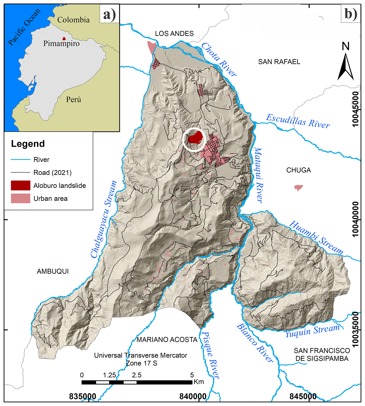
Figure 1 Location of the study area. (a) Ecuador in northwestern South America. (b) Pimampiro parish and the location of the San José de Aloburo landslide. The white circle highlights the landslide area.

Figure 2 Context maps for Pimampiro and the San José de Aloburo landslide. Capital letters correspond to the parish scale and lowercase letters to the landslide area: (A, a) geological context modified from Egüez et al. (2017); (B, b) slope classification after Aramburo and Escribano (2014); (C, c) surface-water features based on IGM mapping; and (D, d) land use and anthropogenic activities based on Prefectura de Imbabura data.

The raster map panels reproduce the coordinate annotations present in the archived map exports. The corresponding GIS project files were not included in the manuscript source package available for this revision, so the underlying coordinate reference system cannot be independently re-derived from that archive. No unsupported numerical reprojection of the raster figures was therefore introduced; the map grids are used only for spatial context and are not used in the ERT inversion or quantitative calculations.

The area lies within the Mira River basin and Chota sub-basin. Irrigated agriculture is a dominant land use, and canals and reservoirs are common in the surrounding terrain (GAD Imbabura, 2017; Mothes, 1987; MAGAP, 2015). These hydrological and anthropogenic elements provide relevant context for infiltration and water redistribution, but the present study does not quantify their direct contribution to the 2021 failure.

3 Data and methodology

The workflow combined geological field observations and ERT acquisition, followed by independent processing and subsequent joint interpretation. Geological information is used as a constraint on the interpretation of shallow geoelectrical patterns rather than as a direct conversion from resistivity to lithology.

3.1 ERT survey design and acquisition

Four ERT profiles were acquired in the upper and accessible sector of the landslide (Fig. 4). The final field geometry differed among profiles because the survey had to be adapted to terrain access, damaged ground, agricultural infrastructure, and the practical limitations of the manual low-cost acquisition system. The final datasets used for inversion had a base Wenner spacing of 5 m for Profile 1 and 7.5 m for Profiles 2–4 (Table 1). The profiles were not parallel: Profile 1 trends NW–SE, Profile 2 N–S, Profile 3 NE–SW, and Profile 4 SW–NE. Profile 3 lies outside the mapped displaced area and is used only as a spatial reference profile, not as a pre-failure measurement.

The Wenner array was selected because of its comparatively strong signal response and suitability for broad, layered resistivity variations with depth. Its lower lateral sensitivity relative to arrays such as dipole–dipole limits the resolution of narrow or steeply dipping structures, and this limitation is considered in the interpretation (Aizebeokhai, 2010; Friedel et al., 2006). For a Wenner array, AM = MN = NB =a and AB =3a. The archived field geometry preserves the maximum a-spacing used for each line: 55 m for Profile 1, 60 m for Profiles 2 and 3, and 37.5 m for Profile 4, corresponding to maximum AB separations of 165, 180, 180, and 112.5 m, respectively.

Table 1 Final acquisition geometry of the four ERT profiles. The reported maximum AB separation is derived from the Wenner geometry AB =3a.

The survey used a low-cost, non-commercial electrical resistivity system developed at Yachay Tech University (Fig. 3). The documented configuration consisted of a 12 V DC battery, a converter producing approximately 220 V AC, two multimeters, a current transformer, stainless-steel electrodes, and 50–100 m cables. Current was injected through electrodes A and B, the potential difference was measured between M and N, and the injected current was monitored with the second multimeter together with the current transformer. Complete archival documentation of the exact injection frequency and waveform, multimeter models and bandwidth/accuracy specifications, current-transformer ratio, field current and power range, number of stacks, and resistor-based calibration procedure is not available. These missing parameters are therefore not reconstructed retrospectively; the resulting limitation on full instrumental reproducibility is stated explicitly in Appendix A.

Figure 3 Low-cost ERT acquisition system. The photographed components are: (1) measuring tape, (2) hammer, (3) 12 V battery, (4) current transformer, (5) 100 m cables, (6) multimeters, and (7) 50 m cables. A, B, M, and N denote the Wenner current and potential electrodes.

Figure 4 Location of the four ERT profiles in the San José de Aloburo study area. The NW–SE arrow shows the principal movement direction documented in the 2021 post-event assessment (Vázquez et al., 2021). The red outline is the landslide boundary used in the project mapping. Because the archived project material does not preserve the complete digitization workflow for this outline, it is used here as a spatial reference rather than as a newly re-derived geomorphic boundary. The base image is a June 2023 drone orthophoto, courtesy of K. Freire.

3.2 ERT processing and inversion

Field readings were digitized in spreadsheets and apparent resistivity was calculated using the Wenner geometric factor,

$$\begin{array}{}\text{(1)}& {\mathit{\rho }}_{\mathrm{a}}=\mathrm{2}\mathit{\pi }a\left({\displaystyle \frac{\mathrm{\Delta }V}{I}}\right),\end{array}$$

where ρ_a is apparent resistivity, a is the Wenner spacing, ΔV is the measured M–N potential difference, and I is the A–B injected current.

The profile endpoints were georeferenced in ArcMap. Electrode positions were generated in QGIS using QChainage and assigned elevations from a digital terrain model so that measured topography could be incorporated into the inversion. Final 2-D inversions were carried out in RES2DINV. The archived methodology indicates that the models were iterated at least three times while data consistency and noisy observations were assessed. Topographic elevations were incorporated into the inversion mesh so that the forward response was calculated for the non-flat surface geometry (Seequent, 2023).

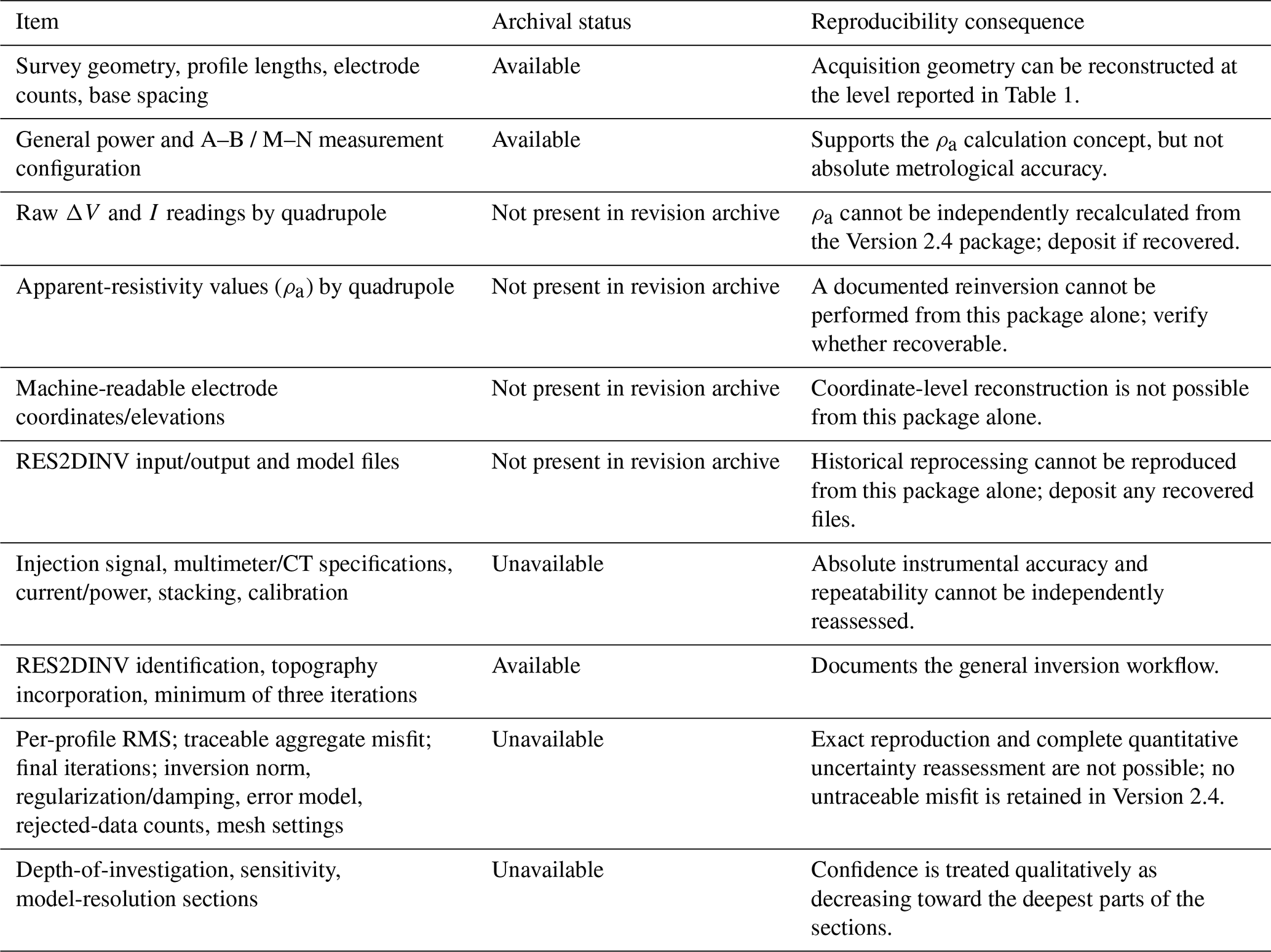
The archived project material does not preserve the information required to reconstruct all inversion settings retrospectively. In particular, per-profile RMS/misfit values, final iteration counts, the inversion norm or constraint type, regularization or damping parameters, the error model, rejected-data counts, and detailed mesh settings are not available in the source package used for this revision. These quantities are therefore reported as unavailable rather than inferred from software defaults. Earlier manuscript versions reported an aggregate mean inversion misfit of 15.78 %, but the current revision archive does not contain the per-profile logs or a traceable source file from which that aggregate value can be independently verified. To avoid retaining an untraceable quantitative quality metric, the 15.78 % value is not used in Version 2.4. This limitation reduces inversion reproducibility and prevents a complete quantitative reassessment of model uncertainty.

The interpretive traces shown on Profiles 1, 2, and 4 were delineated manually after inversion. They follow pronounced resistivity gradients where those gradients are also spatially compatible with the mapped upper-sector morphology and, in the shallow interval, with the available geological observations. No numerical gradient threshold, automated discontinuity detector, or mechanical failure criterion was used to generate these traces. They are therefore interpretive boundaries rather than outputs of the inversion algorithm. Because no archived depth-of-investigation, model-resolution, or sensitivity sections are available for the final inversions, confidence is considered qualitatively lower toward the deepest portions of the sections. This conservative treatment is consistent with the broader ERT literature, in which resolution, model regularization, survey geometry, and decreasing sensitivity with depth constrain how confidently deep electrical boundaries can be interpreted (Balasco et al., 2022).

The four independently inverted 2-D sections were subsequently displayed using a common 16-interval resistivity color scale. They were positioned according to their survey geometry to construct a 3-D fence diagram. No volumetric 3-D inversion or interpolation between the profiles was performed; therefore, the fence diagram is used only to compare the spatial arrangement of the independently inverted 2-D sections.

3.3 Geological field observations and grain-size analysis

Three stratigraphic columns were described around the landslide margins and accessible exposures (Fig. 5). Fieldwork was conducted on 5 September 2024 using a tape measure, grain-size reference scale, compass, and field notebook. The columns document alternating volcaniclastic units, principally fine ash, coarse ash, pumice-rich/lapilli deposits, and reworked units, using the descriptive framework of Gillespie and Styles (1999). Column C had to be located in a nearby stream because the originally planned southern exposure was disturbed by the landslide.

Figure 5 Locations of stratigraphic columns A, B, and C around the San José de Aloburo landslide. The points represent the exposures used to document the local volcanic and volcaniclastic sequence. Base image: Google Earth (©Google; imagery ©CNES/Airbus and Maxar Technologies).

Only one sample, ANG-TOP-B-01, is used for the quantitative sieve analysis reported in this manuscript. Other grain-size descriptions in the stratigraphic columns are field observations. For the quantitative analysis, the sample was manually disaggregated to separate particles while minimizing breakage, weighed, and passed through seven sieves ranging from 2 mm to 85 µm. Retained, cumulative retained, and passing percentages were calculated to construct the grain-size distribution curve. Because the quantitative dataset comprises one analyzed sample, it is treated as local sedimentological information and is not used to establish a site-wide statistical resistivity–grain-size relationship.

4 Results

4.1 Geological constraints

The three stratigraphic columns document a heterogeneous volcanic and volcaniclastic succession (Fig. 6). Column A contains alternating pumice/lapilli-rich and ash-rich units; Column B contains a comparable sequence with multiple ash and pumice levels; and Column C, located south of the mapped landslide, includes thicker units and a coarse-ash level not clearly represented in the other columns. These variations indicate lateral changes in unit thickness and depositional geometry that are relevant when interpreting the ERT sections.

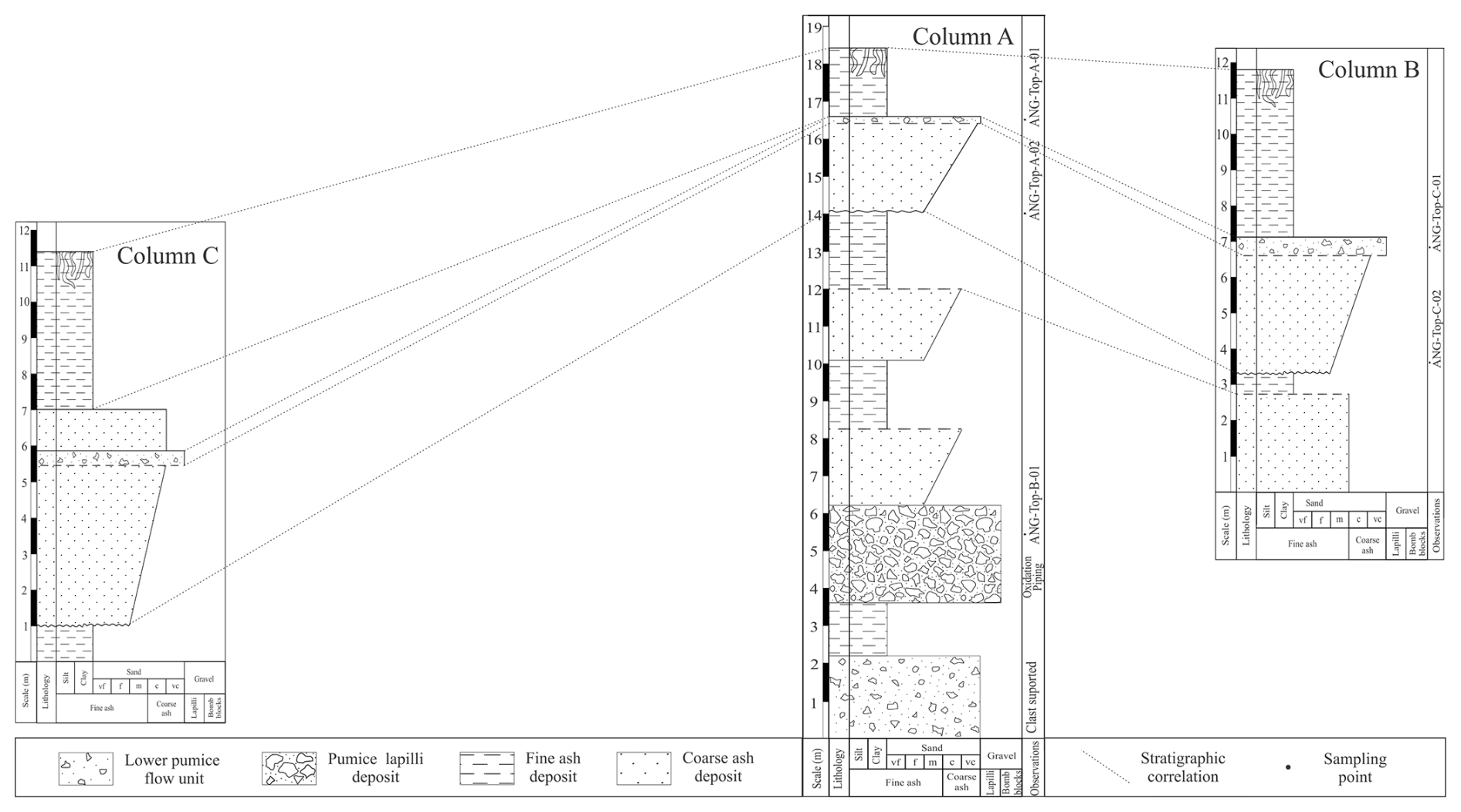
Figure 6 Stratigraphic correlation of columns A, B, and C. The vertical axes in the original field columns represent stratigraphic height measured upward from the local base of each exposure; they should not be interpreted directly as depth below the ground surface. The maximum observed stratigraphic thickness is approximately 19 m, so these columns provide direct geological control only for the shallow part of the ERT sections.

The observed alternation between coarser pumice/lapilli-rich units and finer ash-rich units provides a plausible hydrostratigraphic framework in which permeability and water retention may vary vertically and laterally. Nevertheless, hydraulic conductivity, saturation, pore pressure, and shear strength were not measured directly in this study; the geological observations are therefore used to constrain possible interpretations rather than to demonstrate a specific failure mechanism.

As local sedimentological support, the quantitative sieve analysis of ANG-TOP-B-01 had an initial mass of 396.19 g, with 1.35 % material loss during processing. The largest fractions were retained on the 2 mm (40.28 %) and 1 mm (23.34 %) sieves, whereas only 1.36 % passed the 85 µm sieve (Fig. 7). The analyzed material is therefore predominantly coarse grained and is consistent with a pumice/lapilli-rich volcaniclastic unit containing an ash matrix. This result supports the local field description of the sampled unit but does not validate a general relationship between low resistivity and fine-grained material across the landslide.

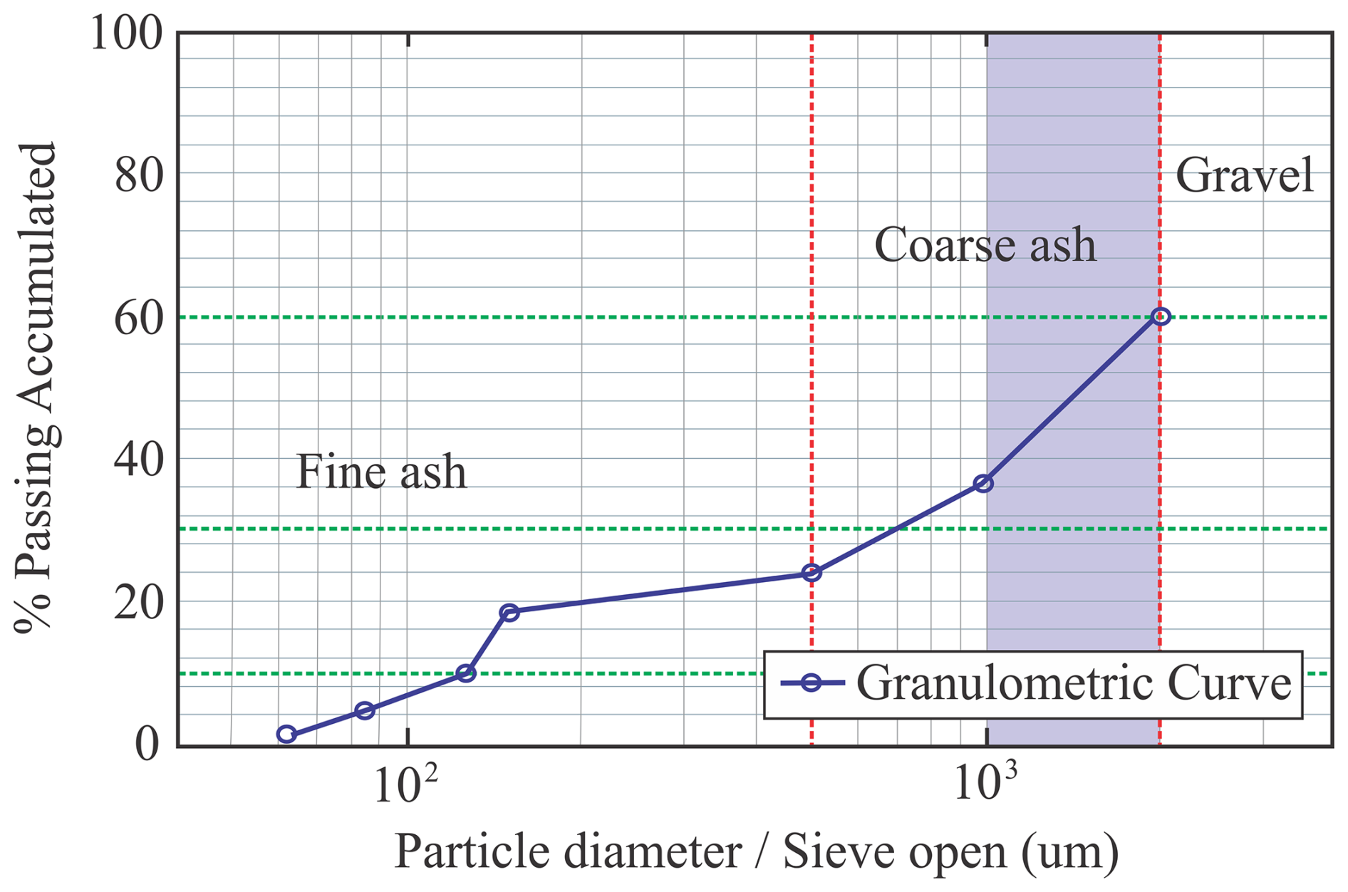
Figure 7 Particle-size distribution of sample ANG-TOP-B-01. The result is used as local sedimentological information only; no site-wide grain-size–resistivity calibration is inferred from this single quantitative sample.

4.2 ERT results

The four inverted ERT sections show broad geoelectrical domains ranging from approximately 4 to 297 Ω m (Fig. 8). Low-resistivity domains (approximately 4–45 Ω m) occupy substantial parts of the sections, while intermediate and higher resistivities occur locally, particularly in Profiles 1 and 2 and toward parts of the profile margins. These patterns are described first as electrical contrasts; their geological significance is evaluated only through comparison with morphology and field observations.

No traceable per-profile or aggregate inversion-misfit metric is retained as a quantitative quality indicator in Version 2.4. The value reported in earlier manuscript versions could not be independently traced to preserved per-profile logs or a source file in the current revision archive and was therefore removed. The manual acquisition system, complex topography, heterogeneous ground, electrode-contact conditions, incomplete instrumental metadata, and incomplete inversion metadata prevent a more detailed quantitative uncertainty analysis. Sensitivity and resolution generally decrease with depth, so the deepest interpreted boundaries are treated as less constrained than the shallow parts of the sections.

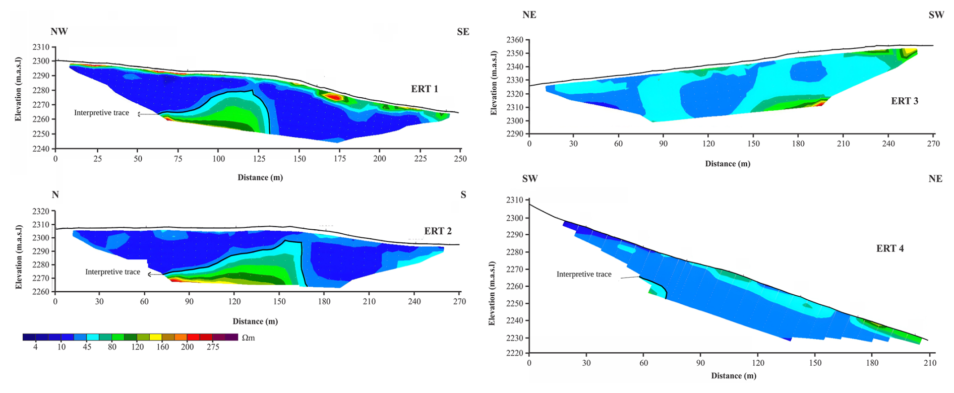
Figure 8 Electrical resistivity tomography profiles. Profile 1 trends NW–SE, Profile 2 N–S, Profile 3 NE–SW, and Profile 4 SW–NE. The black traces in Profiles 1, 2, and 4 are interpretive traces manually delineated from pronounced geoelectrical gradients together with upper-sector morphology and shallow geological constraints; they are not outputs of an automated discontinuity detector and are not independently verified mechanical slip surfaces. Profile 3 lies outside the mapped displaced area and is used as a spatial reference profile rather than as a pre-failure measurement.

Profiles 1 and 2 contain pronounced low-to-intermediate resistivity domains overlain or bounded by locally higher resistivities. In both sections, the manually interpreted black traces coincide with marked resistivity gradients and with the upper-sector morphology. These boundaries occur within an approximate depth range of 10–35 m below the local surface in the inverted sections. Because the available stratigraphic columns extend to only about 19 m, no borehole or inclinometer crosses the deeper boundary, and no quantitative depth-of-investigation assessment is preserved, these traces are interpreted as potential instability-related zones rather than confirmed rupture planes. Their deepest portions should be considered the least constrained.

Profile 3 shows a comparatively smooth distribution dominated by low-to-intermediate resistivity values and is broadly similar to parts of the other profiles. Its similarity is important because it demonstrates that conductive domains are not unique to the mapped displaced area and may reflect regional lithological and hydrological controls. Profile 4, which crosses farther into the mapped upper landslide sector, is also dominated by low-to-intermediate resistivities with localized contrasts. The four profiles therefore document subsurface electrical heterogeneity, but they do not by themselves demonstrate that water accumulation or a single lithological boundary controls the entire landslide.

The profiles mainly sample the crown and upper accessible sector. Consequently, the ERT dataset does not define the full depth, volume, or complete three-dimensional geometry of the approximately 25 ha landslide. Interpretations in this paper are explicitly limited to the surveyed sector.

4.2.1 3-D fence diagram of the 2-D ERT profiles

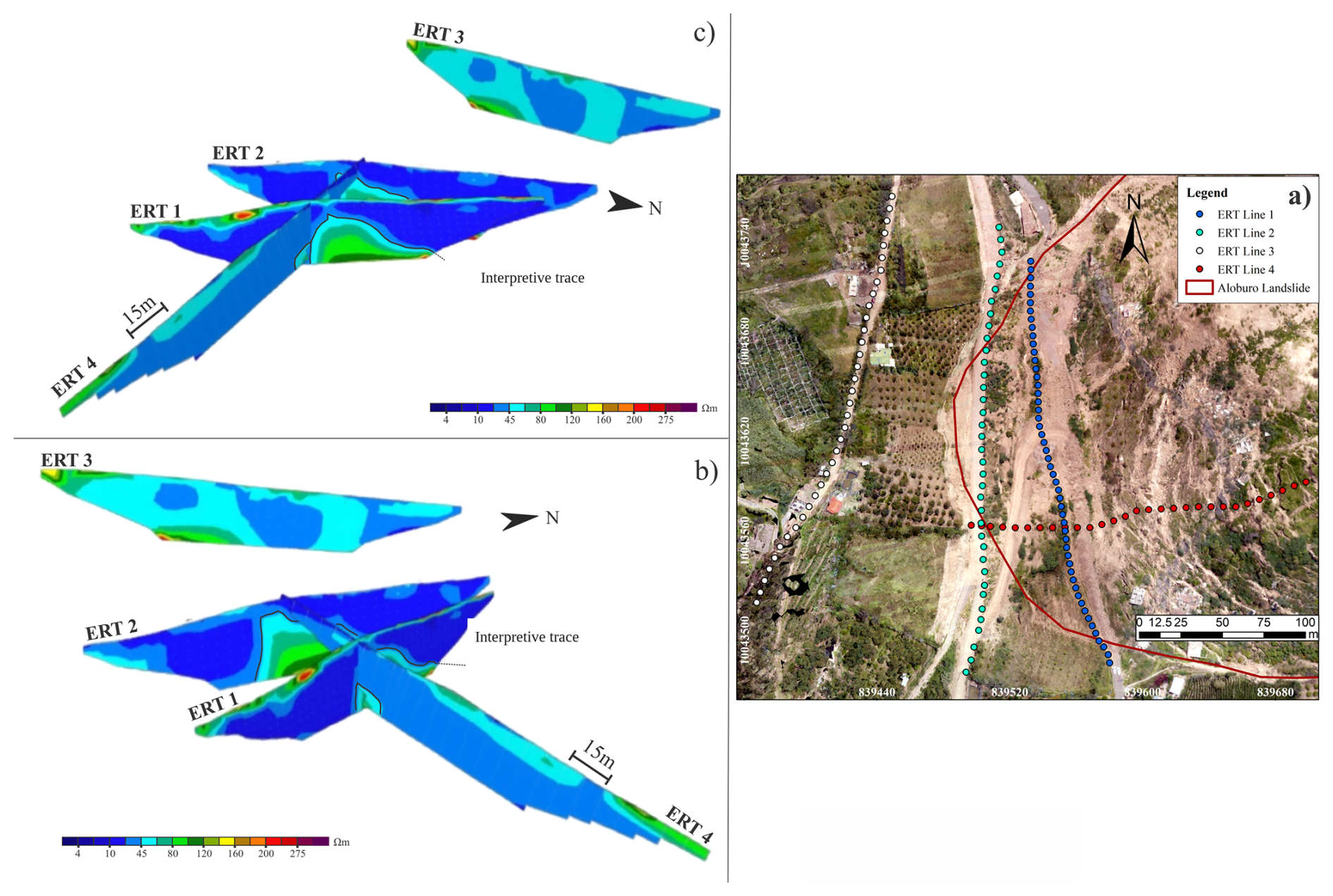
Figure 9 3-D fence diagram constructed by positioning the four independently inverted 2-D ERT profiles in their survey geometry. Panel (a) shows profile locations on the June 2023 drone orthophoto (courtesy of K. Freire); panels (b) and (c) provide two viewing directions. The fence diagram is a visualization for spatial comparison and is not a volumetric 3-D resistivity inversion. The black traces represent interpreted potential instability-related boundaries in the individual 2-D sections.

The fence diagram (Fig. 9) helps compare whether resistivity patterns observed in one 2-D section are spatially compatible with those in another. It does not demonstrate continuous layers or a continuous rupture surface between profiles because no resistivity values were inverted or interpolated in the volumes between the sections. The most defensible use of the fence diagram is therefore qualitative spatial comparison of the independently resolved geoelectrical domains.

5 Discussion

The revised interpretation distinguishes electrical observations from geological inference. Bulk resistivity is controlled by several coupled factors, including mineralogy, grain size, porosity, degree of weathering, water content, and pore-fluid conductivity (Perrone et al., 2014; Whiteley et al., 2019). Therefore, the 4–45 Ω m domains observed at San José de Aloburo cannot be uniquely assigned to saturation, fracturing, or low cohesion. Conversely, a fractured zone need not be conductive if fractures are relatively dry. ERT also does not measure cohesion directly. In this study, low-resistivity domains are consequently described as conductive geoelectrical zones that are consistent with increased moisture and/or electrically conductive volcaniclastic material where the field geology supports such an interpretation.

This cautious approach is consistent with integrated landslide studies in which ERT interpretations are strengthened by independent geological or geotechnical constraints. For example, Friedel et al. (2006) combined 2-D/3-D ERT with penetration tests, boreholes, and laboratory analyses, and showed that wet- and dry-period surveys helped separate hydrological from lithological effects. Bellanova et al. (2018) used resistivity imaging to characterize the Montaguto landslide, while Pasierb et al. (2019) demonstrated the value of integrating ERT with geotechnical data for stability assessment. These studies underline an important limitation of the present dataset: the San José de Aloburo survey has stratigraphic control at shallow depth but no direct geotechnical verification of the deeper geoelectrical boundaries.

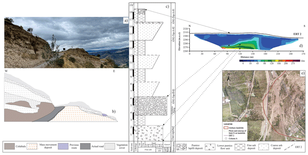
The geological columns are therefore used primarily to constrain the upper part of the ERT interpretation. Their maximum observed thickness is approximately 19 m, whereas the ERT sections extend to approximately 35–40 m. A direct one-to-one correlation between stratigraphic contacts and deeper iso-resistivity contours is not justified. Figure 10 illustrates the spatial comparison among the field exposure, geological sketch, Column A, and Profile 2. Panel (b) is a conceptual sketch and is not drawn to vertical scale; panel (c) records stratigraphic height from the base of the exposure; panel (d) is the independently inverted ERT section; and panel (e) shows their map relationship. The dashed connectors are intended to show approximate spatial correspondence in the shallow sector, not to imply that resistivity contours are geological layer boundaries.

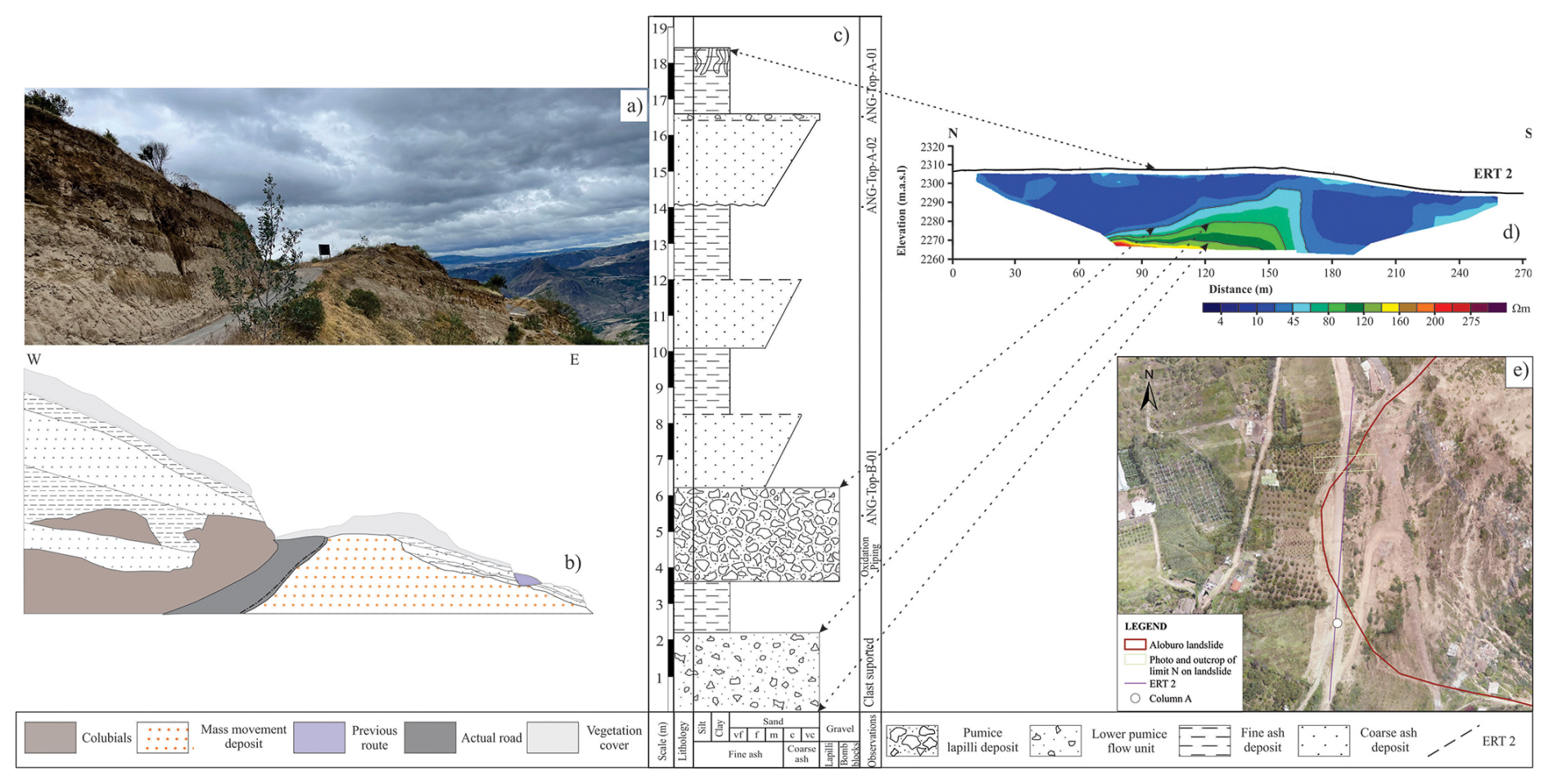
Figure 10 Integration of geological and geophysical observations. (a) Field photograph taken by the authors during the 5 September 2024 field campaign, showing the present exposure and slope conditions. (b) Conceptual geological sketch of the exposed units; the sketch is not to vertical scale. (c) Stratigraphic Column A, plotted as stratigraphic height measured upward from the local base. (d) Independently inverted ERT Profile 2. (e) Location map showing the landslide outline used in the project, ERT Profile 2, Column A, and the approximate position of the photographed outcrop; the base is the June 2023 drone orthophoto (courtesy of K. Freire). The dashed connectors illustrate approximate spatial relationships only and do not equate geological contacts with iso-resistivity boundaries.

The stratigraphy suggests a plausible hydrogeological contrast between coarser pumice/lapilli-rich units and finer ash-rich units. Coarser units may favor infiltration and drainage relative to finer layers, whereas finer units may locally impede vertical flow. Such contrasts could promote perched or laterally redirected water under wet conditions. However, this mechanism remains conceptual because hydraulic conductivity, pore pressure, and water content were not measured directly. The single quantitative grain-size analysis of ANG-TOP-B-01 further limits the strength of any site-wide sediment–resistivity correlation. Its coarse distribution is therefore treated as local sedimentological evidence only.

Seasonality is another important limitation. The principal landslide occurred during the October–December wetter period, whereas the ERT campaign represents later, comparatively drier post-event conditions. The resistivity models should therefore be regarded as a temporal snapshot rather than as a direct reconstruction of the hydrological conditions that prevailed during the November 2021 failure. Seasonal changes in water content and hydraulic connectivity could alter both the amplitude and spatial continuity of conductive anomalies. Time-lapse electrical studies on active landslides demonstrate that repeated surveys can separate persistent electrical structure from transient hydrological changes and can substantially improve interpretation of subsurface water circulation (Uhlemann et al., 2017; Whiteley et al., 2019; Carrier et al., 2024). In debris affected by reactivation, recent ERT work also illustrates both the value of conductive anomalies for identifying water-related zones and the interpretive difficulty that remains when direct subsurface validation is limited (Ullah et al., 2023).

A wet-season ERT survey acquired with the same geometry would consequently provide valuable complementary information. Comparison of wet- and dry-season models could test whether low-resistivity domains expand or become more continuous during infiltration, whether conductive zones persist through both seasons, and whether the interpreted potential instability-related boundaries are spatially stable. No such repeated dataset is available here, so lithological and hydrological contributions cannot be separated quantitatively.

The Wenner configuration also influences the achievable resolution. Its strong signal response is advantageous for manual field acquisition, but its comparatively limited lateral resolution can smooth narrow or steeply dipping structures. In addition, inversion regularization and decreasing sensitivity with depth can broaden or suppress thin units. The approximately 1.3 m layer observed in the stratigraphic record but not resolved in the ERT section should therefore not be interpreted as absent. Its thickness relative to the 5–7.5 m base electrode spacing, potentially limited electrical contrast with adjacent material, and inversion smoothing all provide plausible reasons why it may not appear as a distinct electrical layer.

Recent integrated landslide investigations provide useful context for the level of inference supported by the present dataset. At Montescaglioso, geological observations were combined with multiple geophysical methods to refine the internal landslide architecture (Calamita et al., 2023), whereas geophysical–geotechnical integration in residual soils demonstrates how direct mechanical control can strengthen slip-surface interpretation (Olabode et al., 2022). In the Andes, the Laguna del Amor study in Peru provides a geographically relevant example of ERT integrated with field geology and geomorphology (Zevallos et al., 2025). These studies support the integrated strategy used here, but they also highlight why the present manuscript limits its conclusions where borehole, geotechnical, or repeated hydrological measurements are unavailable.

Finally, the non-commercial ERT system is an important practical component of the study, but its archived metadata are incomplete. The available records document the general acquisition configuration and the measured quantities used to compute apparent resistivity, whereas several electronic specifications and calibration details requested during review cannot be recovered reliably. Consequently, the absolute measurement accuracy cannot be independently reassessed from the archived material, and the missing metadata constitute an unquantified source of instrumental uncertainty. Fully documented low-cost systems provide useful benchmarks for the level of signal characterization, repeatability testing, validation, and open processing that is desirable when instrumentation itself is the principal methodological contribution (Clément et al., 2020; Farzamian et al., 2024; Delmonte et al., 2025). The system used here is therefore presented as the acquisition platform for this case study, not as a fully reproducible instrument design or metrological benchmark, and no performance equivalence with those systems is claimed.

6 Conclusions

The four ERT profiles resolve broad geoelectrical domains in the upper and accessible sector of the San José de Aloburo landslide to approximately 35–40 m depth. Low-resistivity domains of approximately 4–45 Ω m are prominent, but they cannot be uniquely interpreted as saturated, fractured, or low-cohesion material. Their geological meaning is constrained by field morphology and stratigraphy, and selected strong resistivity gradients in Profiles 1, 2, and 4 are interpreted as potential instability-related boundaries rather than mechanically verified rupture planes.

The stratigraphic columns document alternating ash and pumice/lapilli-rich volcaniclastic units and provide direct geological control only within the shallow observed interval, up to approximately 19 m. The quantitative grain-size analysis of ANG-TOP-B-01 confirms a locally coarse-grained volcaniclastic unit but does not validate a general resistivity–grain-size relationship for the whole landslide. The comparison of stratigraphy and ERT is therefore interpretive and spatial, not a one-to-one correspondence between geological layers and iso-resistivity contours.

The survey geometry is concentrated in the crown and upper accessible sector, so the present dataset does not determine the full depth, volume, or complete 3-D geometry of the approximately 25 ha landslide. The 3-D representation is a fence diagram of independent 2-D inversions, not a 3-D inversion. The principal scientific product of this work is therefore the integrated observational ERT–geology dataset and an uncertainty-aware interpretation workflow, rather than a new instrumental benchmark or a complete geotechnical model of the landslide. Future work should prioritize repeated wet- and dry-season ERT using fixed geometry, additional profiles across the central and lower landslide body, and independent borehole, geotechnical, hydrological, or inclinometer control. Such data would allow more rigorous testing of the proposed hydrological and instability-boundary interpretations.

Appendix A: Available documentation and reproducibility limits of the custom ERT system

The low-cost ERT system was a non-commercial prototype developed for academic field applications at Yachay Tech University. The available archived documentation supports the following description: (i) a 12 V DC battery served as the primary power source; (ii) the system converted this supply to approximately 220 V AC for injection through electrodes A and B; (iii) potential difference was measured between electrodes M and N; (iv) injected current was monitored using a second multimeter in conjunction with a current transformer; and (v) apparent resistivity was calculated from the measured $\mathrm{\Delta }V/I$ ratio using the Wenner geometric factor.

The archived project files do not preserve reliable values for the exact injection frequency or waveform, the make/model and full accuracy/range/True-RMS/bandwidth specifications of the two multimeters, the current-transformer ratio, the minimum and maximum injected current and power, the number of repeated stacks per measurement, or the details of a resistor-based calibration/verification test. These values are therefore not estimated or reconstructed retrospectively. The absence of these metadata prevents an independent reassessment of absolute instrumental accuracy and constitutes an unquantified measurement uncertainty. For the same reason, this manuscript does not present the prototype as a reproducible instrument design; it documents the acquisition configuration to the extent supported by the archived records.

Table A1 Archival status of acquisition data, project files, and inversion metadata relevant to reproducibility. “Not present in revision archive” means that the machine-readable item was not contained in the source package used to prepare Version 2.4; its existence elsewhere has not been verified in this revision.