the Creative Commons Attribution 4.0 License.
the Creative Commons Attribution 4.0 License.
 | 15 Oct 2018
Precise DEM extraction from Svalbard using 1936 high oblique imagery
Niels Ivar Nielsen
Frédérique Couderette
Christopher Nuth
Andreas Kääb
Stretching time series further in the past with the best possible accuracy is essential to the understanding of climate change impacts and geomorphological processes evolving on decadal-scale time spans. In the first half of the twentieth century, large parts of the polar regions were still unmapped or only superficially so. To create cartographic data, a number of historic photogrammetric campaigns were conducted using oblique imagery, which is easier to work with in unmapped environments as collocating images is an easier task for the human eye given a more familiar viewing angle and a larger field of view. Even if the data obtained from such campaigns gave a good baseline for the mapping of the area, the precision and accuracy are to be considered with caution. Exploiting the possibilities arising from modern image processing tools and reprocessing the archives to obtain better data is therefore a task worth the effort. The oblique angle of view of the data is offering a challenge to classical photogrammetric tools, but the use of modern structure-from-motion (SfM) photogrammetry offers an efficient and quantitative way to process these data into terrain models. In this paper, we propose a good practice method for processing historical oblique imagery using free and open source software (MicMac and Python) and illustrate the process using images of the Svalbard archipelago acquired in 1936 by the Norwegian Polar Institute. On these data, our workflow provides 5 m resolution, high-quality elevation data (SD 2 m for moderate terrain) as well as orthoimages that allow for the reliable quantification of terrain change when compared to more modern data.
- Article
(10314 KB) - Full-text XML
- BibTeX
- EndNote


The processing, or reprocessing, of historical imagery into digital elevation models (DEMs) and orthoimages enables the extension of time series for long-term geomorphological change analysis (Csatho, 2015; Mölg and Bolch, 2017; Thornes and Brunsden, 1977). One of the main sources of such data is archived aerial imagery from historical photogrammetric surveys (Kääb, 2002; Vargo et al., 2017). The idea of reprocessing data with modern methods is not new and was already laid out by Chandler and Cooper (1989) using what was then “modern”, but is only more relevant now than it was then, with more archival data (easily) available, giving longer time series, and better modern methods. These approaches can also help reconstruct the geometry of objects or features that have since been lost or destroyed (Falkingham et al., 2014).
Processing nadir imagery over mostly stable land areas where good-quality modern data are available for reference has proven easily accomplished and effective (Baldi et al., 2008; Fox and Cziferszky, 2014; Gomez et al., 2015). However, compared to the processing of modern digital imagery, it must be noted that the task of processing scanned film imagery does come with added challenges.
-
The scanning usually does not conserve a consistent internal geometry (the fiducial marks are not consistently found at the same pixel coordinates), and the images therefore need their internal orientation to be standardized.
-
No metadata are present in the files. If not always strictly necessary, it is often very helpful to have access to (1) calibration information (i.e., calibrated focal and position of fiducial marks) and (2) location information in the form of ground control points (GCPs) or navigation data.
-
Stereo overlap is low (typically 60 % along-track and 20 % cross-track) compared to modern standards (typically around 80 % along-track and 60 % cross-track).
Challenging scenarios are, however, common when metadata are impossible to find or image quality is particularly bad. For instance, large datasets over Antarctica include regions with very little off-glacier stable areas to provide sufficient GCPs, as well as large areas of low-contrast snow fields yielding no tie points and bad or no correlation (Child et al., 2017).
Another common type of imagery is oblique imagery. It was acquired primarily in areas previously unmapped or only superficially so. Such imagery has the advantage of providing a point of view that is easier to comprehend for a human user, and identifiable points can be seen from long distances (even if the image resolution decreases with distance from the camera position). However, for both analytical and computer-based processing, oblique data add a layer of challenges compared to nadir imagery.
-
The footprint of each image is not very well defined as it extends to infinity in a cone shape and excludes part of the ground because of terrain occlusion (e.g., behind ridges and peaks). Therefore, the term viewshed is employed here instead of footprint.
-
The resolution of the imagery is dependent on (1) the distance to the camera (the further away the camera, the lower the resolution) in a much bigger way than nadir imagery (here, the variation in the camera-to-ground distance can vary several fold!) and (2) the slope of the terrain (slopes facing the camera will have a very high number of pixels per horizontal unit of surface).
In this paper, we present and discuss the challenges and solutions related to the processing of oblique (e.g., non-nadir) historical imagery using the 1936 survey of the Svalbard archipelago as an example. We then provide some concise comments on the observed change in elevation over glaciers and rock glaciers.
In the summers of 1936 and 1938, Norwegian expeditions lead by Docent Adolf Hoel went to Svalbard to photograph the area from the air. Bernhard Luncke was in charge of the planning and acquisition of aerial photographs. Their goal was to collect images suitable for creating topographic maps of Svalbard in 1 : 50 000 scale and contour intervals of 50 m (Nuth et al., 2007). The Norwegian Navy provided the expedition with an MF11 scout plane with crew. A Zeiss camera (film format 18×18 cm, focal length 210.71 mm) was mounted in a stabilizing cradle at the side of the plane. The photographs were taken at an altitude of around 3000 m along the coast and 3500 m inland, with the optical axis of the camera pointed 20∘ below the horizon, or 70∘ off-nadir, making them high oblique (Luncke, 1936). The overlap between two images is approximately 60 %.
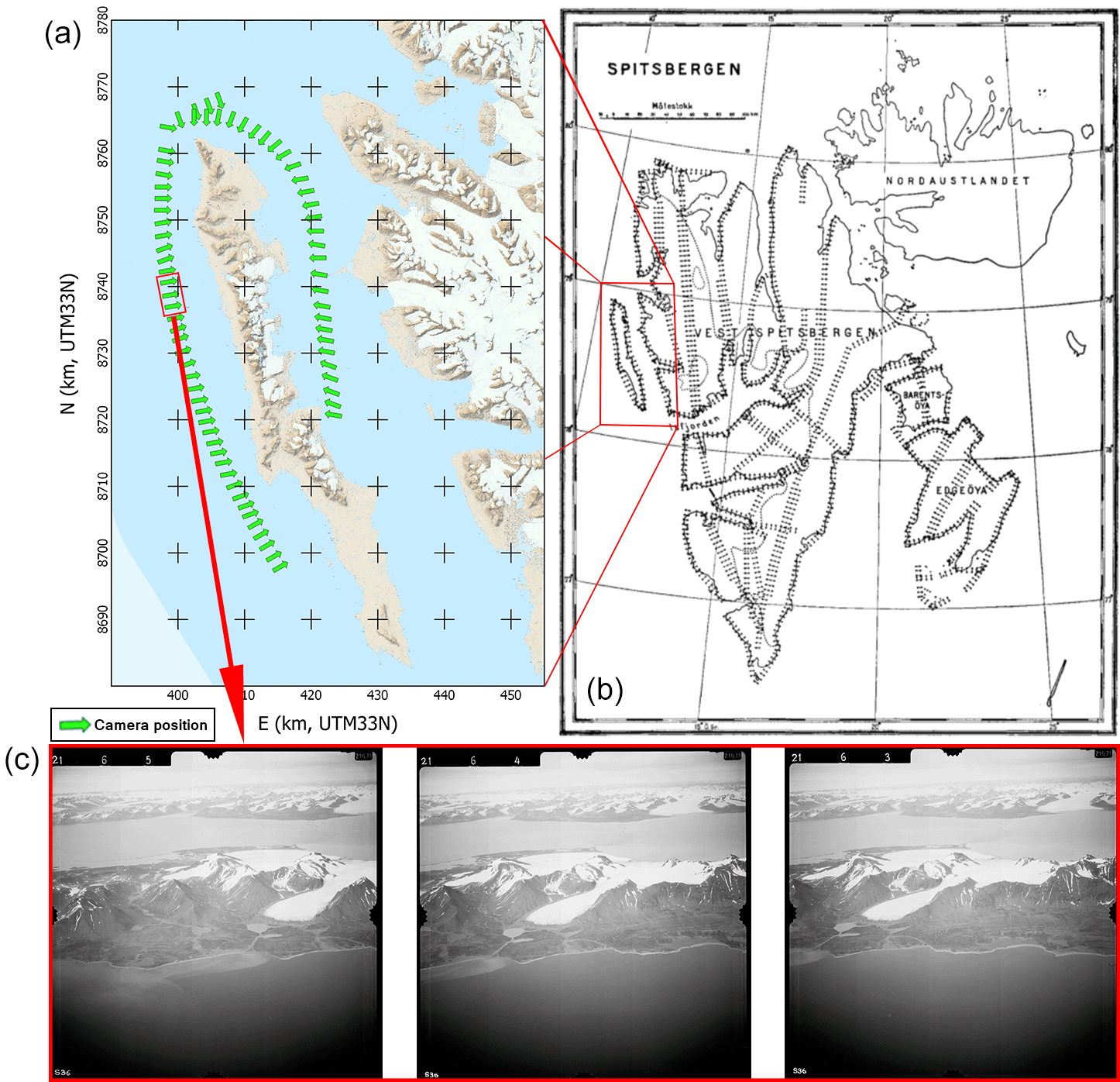
In 1936, good weather conditions allowed for a total effective flight time of 89 h. 3300 images covering an area of 40 000 km2 or nearly 2∕3 of the total area of Svalbard were taken. The areas covered were Barentsøya, Edgeøya, and most of western Spitsbergen. Figure 1 shows where aerial photographs were taken during the 1936 expedition (Luncke, 1936).
The goal of the 1938 expedition was to photograph the areas that were not covered in 1936. Bad weather conditions and technical problems prevented the completion of the planned acquisition, but 48 h of flight time resulted in 2178 photographs covering a total area of about 25 000 km2. In total the two expeditions in 1936 and 1938 resulted in 5478 high oblique aerial photographs that cover most of Svalbard.
The photographs are owned and managed by the Norwegian Polar Institute (NPI).1 In the 1990s, the institute hand digitized the maps made from the data, and in 2014, the original films were scanned with a photogrammetry-grade scanner at a 13.5 µm resolution, resulting in 14 500×14 500 pixel image files. The first attempt at processing the data into native DEM (not computed from map data) using a photogrammetric workstation was made by Etzelmüller and Sollid (1996) over the Erikbreen glacier. Other processing of subsets of the imagery was attempted by Midgley and Tonkin (2017), using three images over Midtre and Austre Lovénbreen, and Mertes et al. (2017) using 25 images over Brøggerhalvøya.
In this paper, a subset of 72 pictures taken in the summer of 1936 in two lines along the western (43 pictures) and eastern (29 pictures) coasts of the Prins Karls Forland, eastern Svalbard, was used as an example (see Fig. 1). The island is a thin band of land covered for the most part by a linear mountain range and some strandflats in the south (not covered by this study). Alpine, marine-terminating, and rock glaciers are present in most of the valley of the island. Some of the illustrative figures in this paper are taken from Nielsen (2017), who used images over Barentsøya (SE Svalbard). As ground truth and as a source of GCPs (see Section 3.4), we used the NPI DEMs from 1990 and 2008 and the TanDEM-X IDEM from 2010.
Historical oblique imagery can be processed through a nearly unmodified typical structure-from-motion photogrammetric pipeline, as described in this section and in Fig. 2. The processing presented in this paper was performed using the open source photogrammetric suite MicMac (Rupnik et al., 2017) (see also http://micmac.ensg.eu, last access: 8 October 2018, for more information).
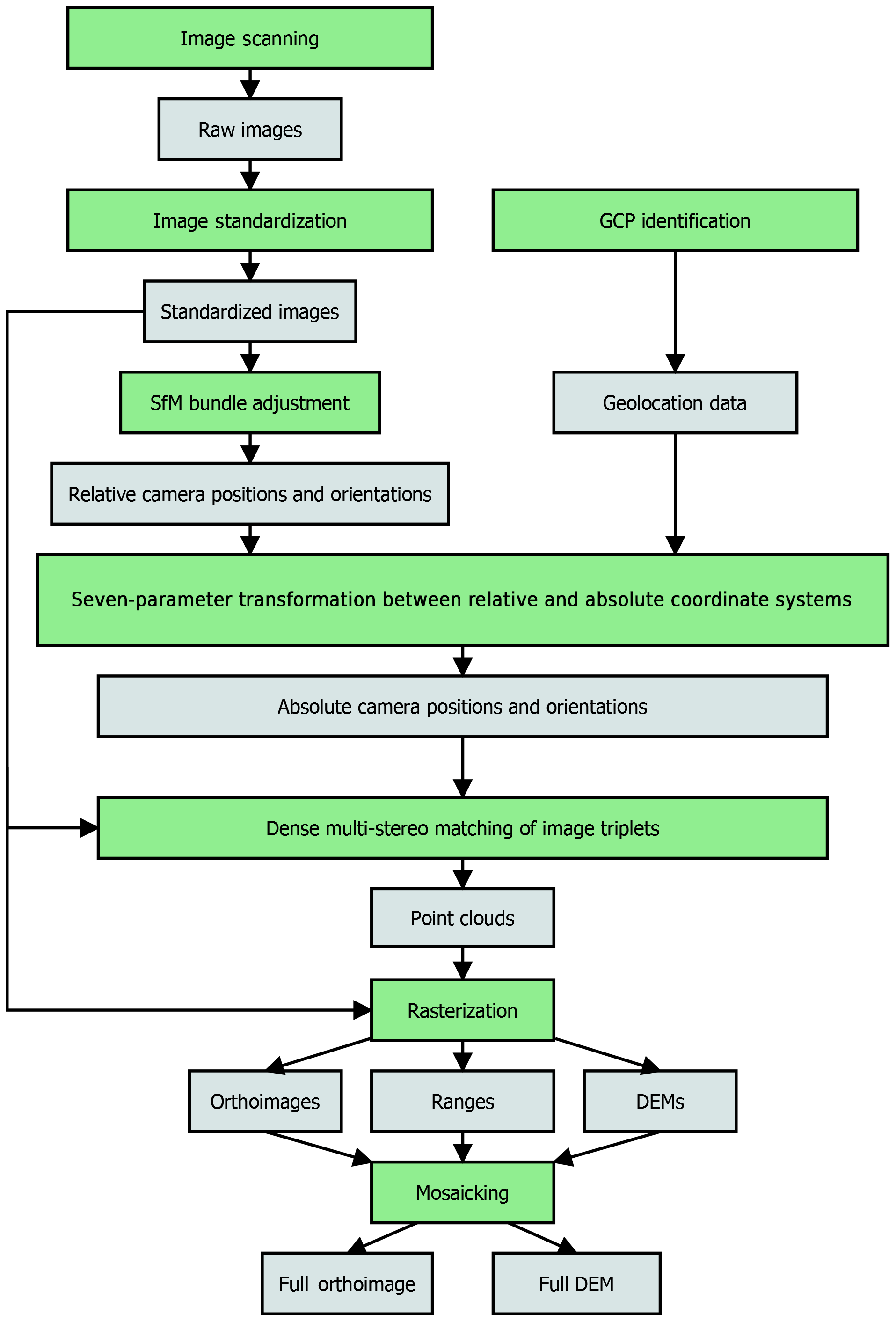
Figure 2Workflow of the structure-from-motion photogrammetric pipeline used in this paper. Data are represented in gray and processes in green.
3.1 Scanning and standardization of the interior orientation
The scanning of images usually results in images that are not all the exact same dimension, and fiducial marks are not necessarily positioned exactly at the same place. To simplify the image assimilation into the photogrammetric process, the interior orientation needs to be standardized: the images have to be geometrically standardized to all be in the same geometry so that the image resolutions and fiducial mark positions are the same, and the internal calibration of all the images is the same (McGlone et al., 2004). Calibration data on the real metric coordinates of the fiducial marks may be available, but an estimate from the size of the film and the relative position of the fiducial marks should be sufficient. In any case, calibration performed on the camera at the time of acquisition would not be taking into account the aging process that the film experienced before having been scanned.
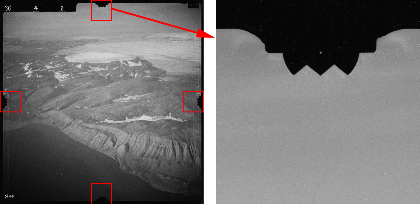
In order to compute the parameters of the 2-D-transformation (translation, rotation, and scaling) for each image, the fiducial marks need to be identified either manually or through an automated process. If fiducial marks are in the center inside of a clear target such as a cross, it is easy to find them automatically. However, this is not the case for our data, in which the fiducial mark is a single dot in the film (see Fig. 3). Using the shape of the frame, it is possible to approximate the position for this point, and then it is possible to identify the brightest circular blob (i.e., the fiducial mark) and record its position (Nielsen, 2017). Once fiducial marks are recorded for an image, it can be resampled in a standardized geometry defined by the user by a bounding box and a virtual scanning resolution.
3.2 Tie point extraction
To be able to run a structure-from-motion-based bundle adjustment, tie points need to be extracted from the imagery. The SIFT algorithm (Lowe, 2004) proved efficient at finding such tie points between adjacent images on land areas, even in the background of the images, hence also providing tie points between images that are not directly adjacent. Typically, SIFT found between 1000 and 10 000 tie points per image, depending on the proportion of contrasted area on the image and the position of the image in the strip. However, SIFT cannot provide tie points between two images if the view directions are too different (over 30∘), which complicates the automatic relative orientation of large groups of images since images taken from two different flight lines usually do not satisfy this requirement. For instance, images from the two opposing lines of flight used in our test case over Prins Karls Forland have an angle between the lines of sight of . Tie points could be identified manually, but unless hundreds could be identified, their contribution to the bundle adjustment would stay weak, potentially leading to a skewed relative orientation. Therefore, in many cases, each flight line needs to be processed individually until the final mosaicking step (see Sect. 3.7).
3.3 Relative orientation and calibration
Once the images are in a coherent internal geometry and the tie points are extracted, the camera can be calibrated and a bundle adjustment process can be performed. The NPI archives contained a single piece of information about the camera used for our data: its focal length of 210.71 mm. From this information, we could initialize the calibration process. The calibration (in the form of Brown's distortion model, Brown, 1966, 1971) is initialized on a small subset of five images that present a good amount of tie points and that are well distributed in the images, thereby covering most of the image field. The remaining images are then added to the block while keeping the camera calibration fixed to obtain a relative orientation of the image set.
3.4 Absolute orientation
The absolute orientation requires GCPs, but no such points were recorded at the time of acquisition in 1936. It is therefore necessary to rely on modern data coverage of the area from which to gather GCPs. To do so, prominent points in stable areas are identified both in the historical images and in a modern source. For our case study, at the time of processing the orientation, the 1990 DEM from the Norwegian Polar Institute represented the best data available and was therefore used. The GSD is 20 m and the SD with the 2008 DEM is below 2 m.
This step is very challenging since most of the lowlands, on top of being generally unrecognizable by a lack of strong structures, cannot be considered stable over 50 years: ice-cored moraines and permafrost areas, thermokarst processes, unstable cliffs, or simply erosion renders the lowlands unstable. Some areas are also challenging to recognize because of the vastly different ice cover over the terrain. Therefore, only bedrock features can be used and it is easiest to identify the mountain tops as GCPs, but even these points are not always very accurate, as the reference DEMs can be of low resolution and often soften the mountain ridges and peaks in particular. The process is further complicated by the strong obliqueness of the historic imagery, making the task of recognizing even very prominent features difficult. The automation of the process used by Vargo et al. (2017) of finding tie points between modern georeferenced images and historical images is impossible to put in action here as no modern images taken in a similar configuration are available. The possibility of misidentification involves the requirement of more GCP candidates that can a posteriori be corrected or filtered out.
Once GCPs are identified, a similarity transformation (seven parameters: three for 3-D translations, three for rotation, and one for scaling) is computed first, and then the camera calibration is reestimated using the GCPs.
3.5 Point-cloud generation
To generate point clouds, images are grouped into triplets of subsequent images in a line of flight. There is no point using more than three images as the area imaged in the central image of a triplet (used as the master image) will not be seen on further images because of the ca. 60 % overlap. Each triplet goes through a dense correlation process (Furukawa and Ponce, 2010; Rupnik et al., 2017) performed in image geometry: a 3-D point in the ground coordinate system corresponding to each pixel in the master image is estimated.
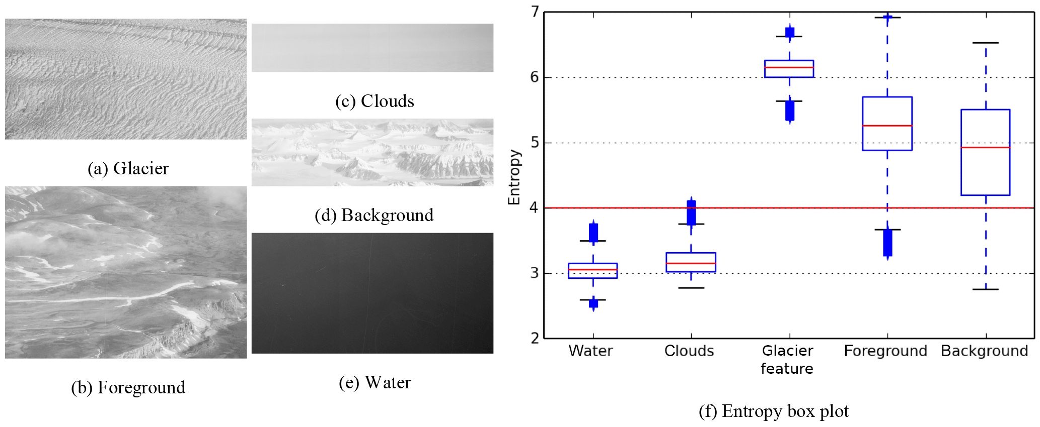
In order to only compute data on areas of interest (in our case, the strip of land closest to the camera positions), the master images need to be masked, as trying to get data out of the entire viewshed area would make the process slower, add noise to the data, and create heavier files that are harder to work with. Specifically, one should mask the sea, the sky, clouds, and background land visible in the image but not in the area of interest. The masking can be completely manual, but it is then a very time-consuming task, especially for large datasets. It is possible to automate the detection of sea, sky, and clouds by running an entropy-based texture analysis, but differentiating foreground and background is more difficult (Nielsen, 2017) (see Fig. 4). Additional masking through the use of a polygon defining the area of interest in ground coordinates is also possible, either by back-projecting a known DEM of it into the individual, then-known image geometries or by filtering out-of-area points during the iterative dense correlation process. These latter approaches were not used in our case study.
3.6 DEM and orthoimage generation
Once a three-dimensional point cloud has been generated, it can be filtered to remove noise and then turned into a number of different raster (2-D) files. The first step in the filtering is to simply remove points that are outside of the area of interest (defined by a polygon in X and Y) and that have a Z component outside of the known minimum and maximum altitudes in the area (with a small margin of error to compensate for imperfect georeference). Noise filtering is then performed to remove local outliers. However, a third pass, manual this time, is still necessary in most cases, as some elements of the terrain such as mountain ridges or the seashore can be a source of erroneous data in the form of rays or fans of points in the approximate direction of the optical rays (see Fig. 5).
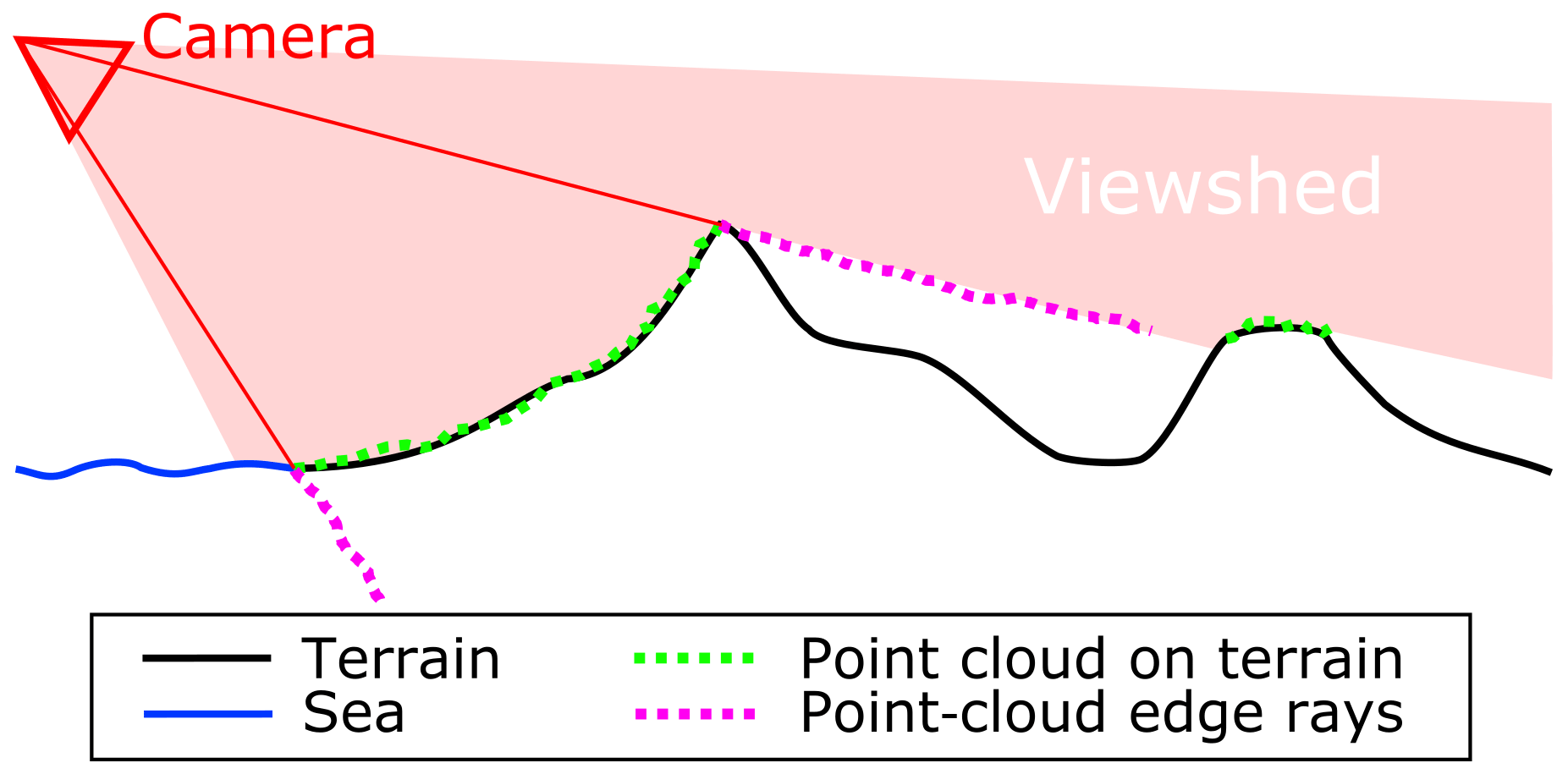
Figure 5Representation of erroneous data points created by mountain ridges and seashore in the approximate direction of the optical rays. Note that the terrain occluded by the foreground mountain, and therefore not included in the viewshed, is not represented in the point cloud.
The clean three-dimensional point cloud is then used as the input for raster data creation. The resolution and corner coordinates of the raster needs to be determined first. From the 1936 Svalbard photos, a 5 m GSD product can be reliably generated in the areas presented in this paper without requiring extensive void filling. Here, we want to create an orthoimage (a raster of colors, here gray scales; see Fig. 6a), a DEM (a raster of elevation; see Fig. 6b), and a record of the distance between the points and the camera (range, see Fig. 6c, to be used later in the mosaicking process, see Sect. 3.7, and as an indication for error propagation). Here, each cell of the rasters is given the mean value of the points in a radius around the cell center.
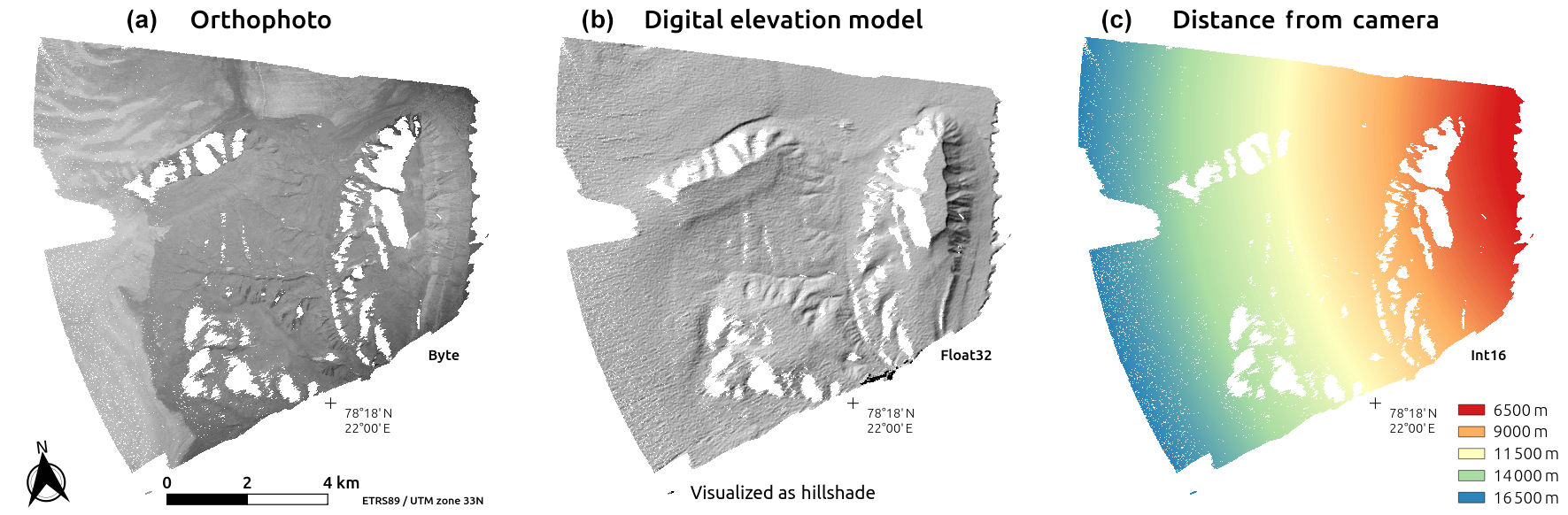
Figure 6Rasters extracted from a single point cloud. (a) Orthoimage. (b) Hillshade of the DEM. (c) Distance to the camera.
3.7 DEM and orthoimage mosaicking
Once all rasters are generated for each point cloud, they can be mosaicked using the distance raster as an input for the creation of a Voronoï diagram: for each point of the final raster, the color and elevation from the set of rasters presenting the lowest range value (distance to camera) are selected and recorded, creating the data shown in Fig. 7.
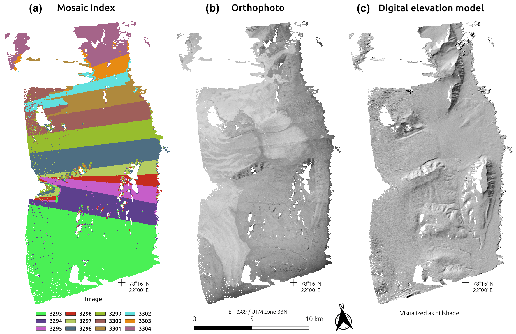
Figure 7Raster mosaic. (a) Map of the mosaic, with each color representing an individual source-point raster. (b) Mosaiked orthoimage. (c) Mosaicked hillshade DEM.
This simple approach creates visible boundaries between each area, especially in the orthoimage, and one might want to perform some radiometric equalization. The mosaicking could be avoided by first merging all the point clouds and performing the rastering process only once from the full combined cloud using a weighting system based on the point-to-camera distance value. However, given that individual clouds can be composed of over 50 million points, the amount of memory required to load dozens of clouds into software (either for merging or rastering) is an almost impossible task, even for a heavy workstation.
In this section, we first discuss the final product quality and then point out the weaknesses remaining in the data that required manual filtering. Figure 8 shows an overview of the output data for the Prins Karls Forland dataset.
4.1 Data quality
A first approach to determine the data quality is to check the residuals of the orientation. Here, after using GCPs to reevaluate the calibration, the average residual of the tie points was 0.803 pixels, and the GCP reprojection error was of 4.108 pixels with an RMSE of 18.15 m. The relatively high RMSE value is most likely due to the relatively soft DEM used as an input for GCP identification. The quality of the data is better estimated by pulling statistics from various differences of DEMs (DoD) between our data and ground-truth DEMs.
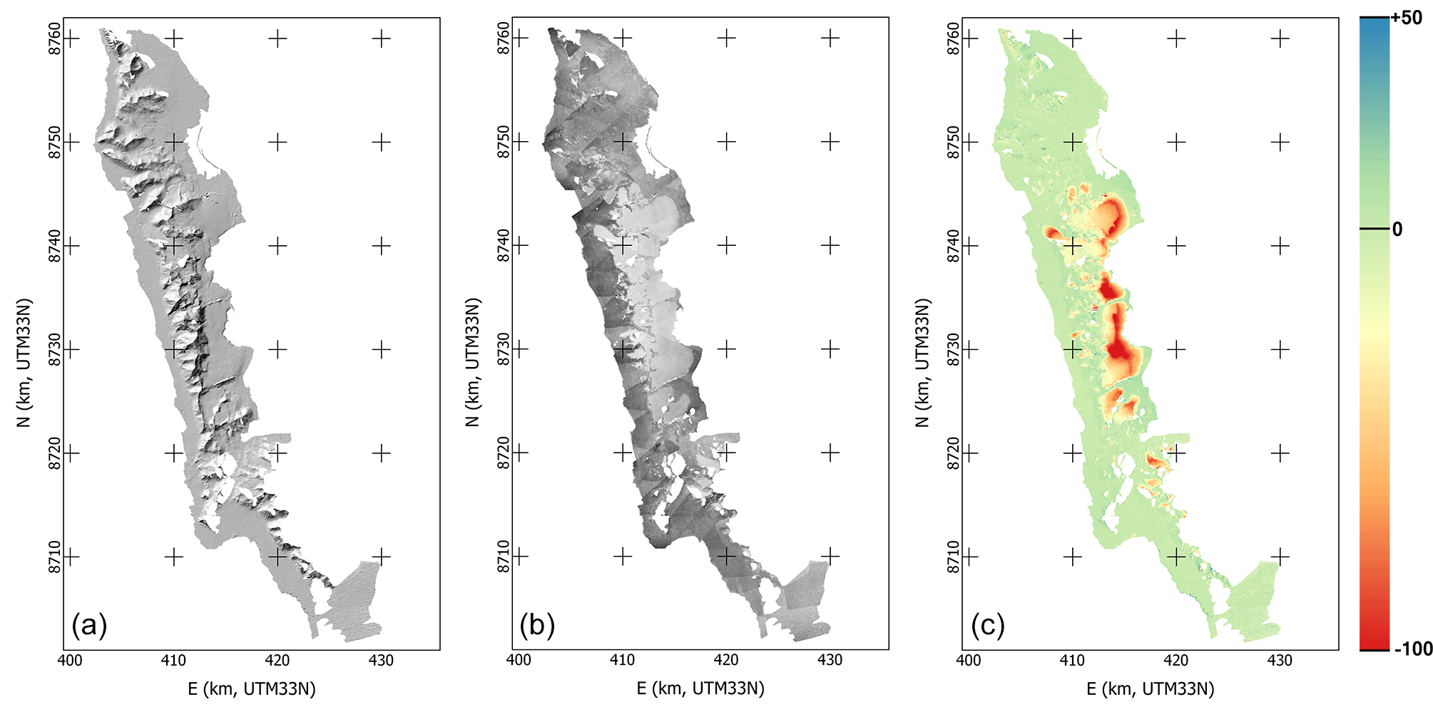
Figure 8Overview of the data resulting from the processing of the 1936 images over Prins Karls Forland. From left to right: Hillshade, orthoimage, DEM difference with the NPI 2008 DEM.

Figure 9Data over Millerbreen. (a) dDEM between our 1936 and the NPI 2008 DEM and profile line (in green). (b) Orthoimage from our 1936 data. (c) Profile data from the dDEM and both 1936 and 2008 DEMs, with the data from the original 1936 map contour lines as red crosses. (d) Map by NPI made using the 2008 data.
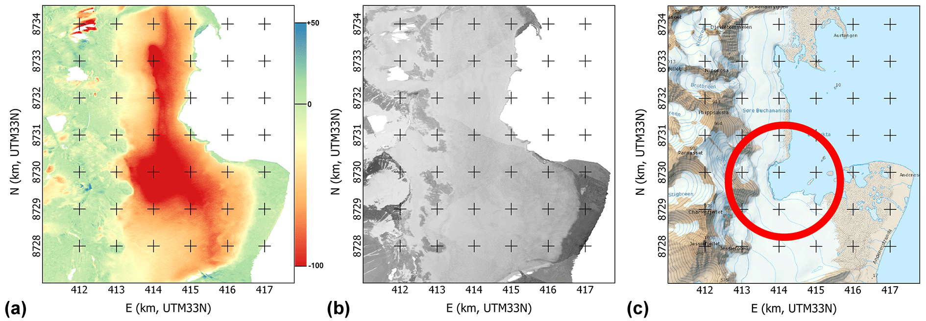
Figure 10Data over Søre Buchananisen. (a) dDEM between our 1936 and the NPI 2008 DEM. (b) Orthoimage from the 1936 data. (c) Map by NPI made using the 2008 data (rectangular indent circled in red).
In order to determine their accuracy, our 1936 elevation data were compared to other DEMs. The NPI most modern DEM product (S0 product) over the area is extracted from the 2008 aerial survey of Svalbard and is also at 5 m GSD. It has a declared accuracy of 2–5 m (https://doi.org/10.21334/npolar.2014.dce53a47). Other data used in comparisons are the NPI 1990 DEM (20 m GSD) and the 2010 TanDEM-X IDEM product (12 m GSD), which is of acceptable quality over the area, except for west-facing steep slopes, for which obvious outliers and data voids are present. This is due to the view angle of the radar satellite that was from the east (descending) during the acquisition. Comparison with the NPI 2008 product on low-slope (<20∘), relatively stable areas that do not present obvious errors returns a standard deviation for the elevation errors of 2 m, while selecting a larger zone containing diverse terrain yielded a value of 5.4 m.
These values are significant improvements on the 12.2 m reported by Nuth et al. (2007) in the comparison of the digitized 1936 map DEM with the 1990 NPI DEM. It is also better than the 5.2 m value reported by Mertes et al. (2017) obtained by comparing the NPI 2010 DEM with the data obtained over Brøggerhalvøya, only over filtered stable ground. Midgley and Tonkin (2017) processed a subset of three images of the Brøggerhalvøya series used by Mertes et al. (2017), hence representing a relatively small area, and reported similar values: 2.9 m for the relatively flat pro-glacial area and 8.5 m when mountain slopes were included in the analysis. While the areas used by both Midgley and Tonkin (2017) and Mertes et al. (2017) for accuracy estimation are not the same as ours, they are described as representing similar type of terrains at a similar distance to the cameras as our areas and hence are a valid comparison.
4.2 Selected geomorphological highlights
The key reason to process the 1936 photos using modern technology is that the result can be used as a baseline to assess long-term change related to glacial and periglacial processes, adding important early data points in the time series of DEMs over the area. By comparing these data with modern products, a nearly centennial glacier mass balance could be estimated, for instance. We show here three examples of different processes observed in the differential DEM (dDEM) between our product based on the 1936 imagery and the most recent DEM from the NPI computed from imagery from 2008.
4.2.1 Alpine glacier example: Millerbreen
In this example, we show the data gathered for the alpine glacier Millerbreen. In 1936, it was land terminating, reaching nearly to its moraine, while in 2008 (and up to today), a large part of the front calves into a lake that formed inside the barrier formed by the moraine. Figure 9 shows the dDEM over the glacier and a profile line over the two DEMs and the dDEM. We can see that during the 72 years separating the two datasets, the glacier retreated by approximately 900 m (12.5 m year−1), losing up to 95 m of ice thickness. The dH curve is very typical for a retreating glacier, linearly going from zero at the old tongue edge to a maximum loss at the new tongue edge and then reaching back to zero at a slower rate up to the top edge of the accumulation zone.
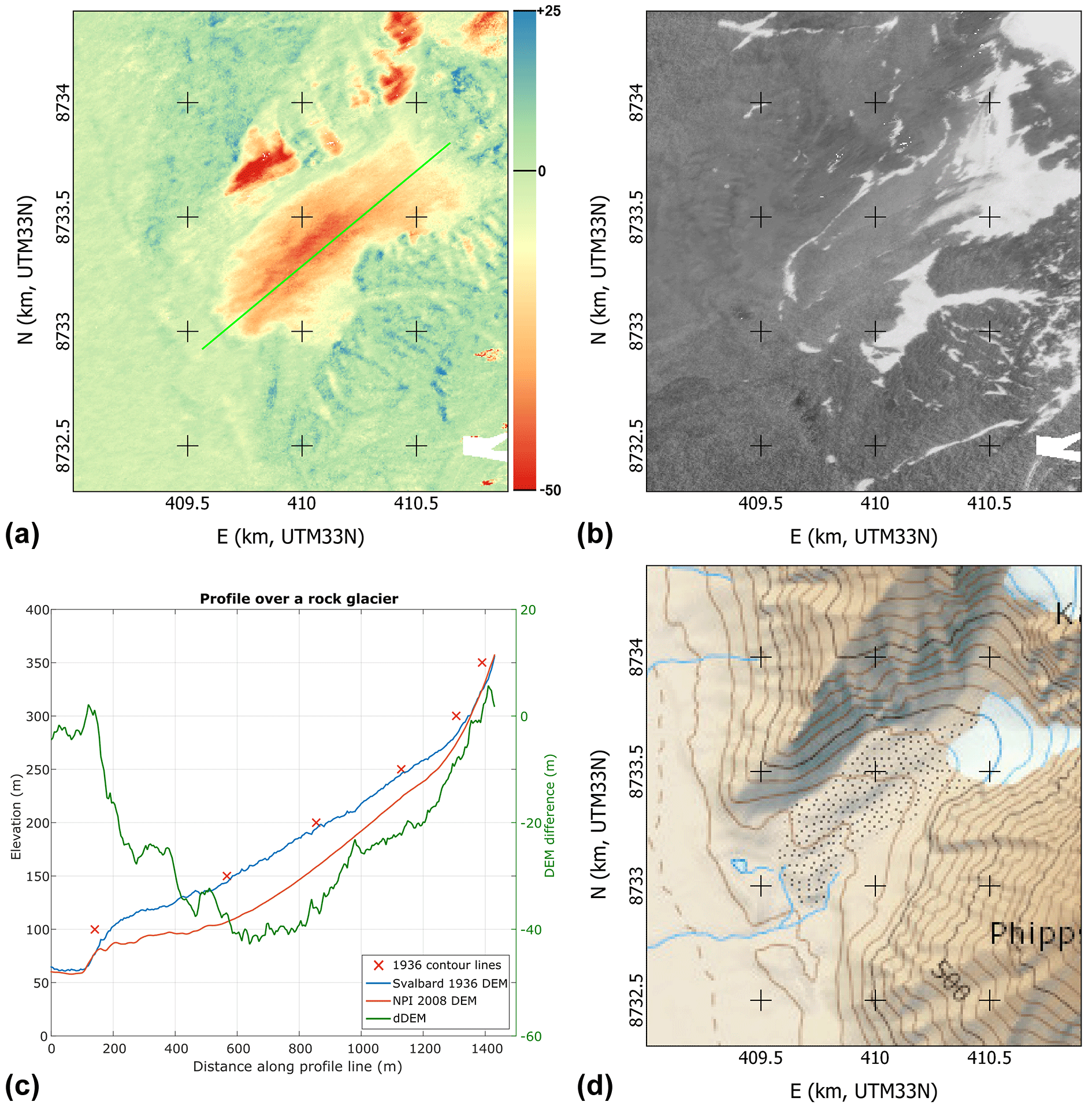
Figure 11Data over an unnamed rock glacier. (a) dDEM between our 1936 and the NPI 2008 DEM and profile line (in green). (b) Orthoimage from our 1936 data. (c) Profile data on the dDEM and both 1936 and 2008 DEMs, with the data from the original 1936 map contour lines as red crosses. (d) Map by NPI made using the 2008 data.
4.2.2 Marine-terminating glacier example: Søre Buchananisen
Søre Buchananisen is a large marine-terminating glacier that experienced a significant retreat (up to 2.0 km) in the 72 years separating the two datasets (27.8 m year−1). The dDEM shows the new ice edge very clearly as the elevation loss is total in the retreated area and only partial from the edge of the ice cliff upwards. The change in the glacier seems to display several basins, with the northern and southern parts retreating fast, separated by a (now) land-terminating middle section. The southern part itself seems to experience contrasting behavior, with the land-terminating part retreating at a significantly lower rate than the marine-terminating front. A quite sharp rectangular indent in the glacier front is visible (see the red circle in Fig. 10c), nearly separating the two parts of the glacier in the 2008 data and still progressing according to the 2010 IDEM data.
4.2.3 Rock glacier example: unnamed, between the peaks of Monacofjellet and Phippsfjellet
The precision of the data allows for a clear identification of rock glaciers (or ice-cored moraines, or small debris-covered glaciers) and of their changes linked to a degradation process. The example shown here for illustration (Fig. 11) exhibits a maximum elevation loss (≈40 m) a third of the way up the landform. The rock glacier front is also flattening (peaking at ≈60 m over the valley bottom in 1936, ≈50 m in 1990, and ≈40 m in 2008). These two observations point to significant ground-ice loss over the 72-year observational period and a topography slowly transforming the whole formation into a talus without abundant ice content.
The value of the information contained in historical photogrammetric surveys for the study of change in the cryosphere is very obvious, as shown by the increasing amount of scientific literature on the topic. With our processing workflow, we achieve an almost fully automated generation of high-quality DEMs even from high oblique photographs. However, such processing still requires some amount of manual work, mostly for GCP identification and for point-cloud cleanup. This cleanup, while crucial to avoid having to deal with areas of vastly erroneous data, does not modify the points that are conserved in the final data and as such does not induce additional noise or noise reduction. Applied on the imagery taken over Svalbard in 1936, our workflow provides high-quality elevation data (STD 2 m for moderate terrain) that allows for the reliable computation of elevation change when compared to more modern data. This may provide an accurate estimate of the retreat and geodetic mass balance of glaciers in the area for the time period since 1936, pushing the beginning of the time series much earlier than previously achievable. The high precision of the data obtained with our workflow also allows for the long-term monitoring of processes presenting elevation changes of smaller magnitude, such as on rock glaciers.
Original imagery from NPI. DEM data available upon request.
LG led the research, wrote the paper, processed the data on Prins Karls Forland, and supervised the work of NIN and FC. FC did an initial assessment of the imagery data and of the potential quality of the products created from them and designed a first version of the workflow (Couderette, 2016). NIN continued that work and automated most of the process (Nielsen, 2017). CN and AK co-supervised the work of NIN and FC, contributed discussions, and edited the paper.
The authors declare that they have no conflict of interest.
The study was funded by the European Research Council under the European
Union's Seventh Framework Program (FP/2007-2013)/ERC grant agreement
no. 320816 and the ESA projects Glaciers_cci (4000109873/14/I-NB), DUE
GlobPermafrost (4000116196/15/IN-B), and CCI_Permafrost (4000123681/18/I-NB).
Data scanning and distribution was funded by the Norwegian Polar Institute.
Couderette's internship was financed in part through the Erasmus program. We
are very grateful to the Norwegian Polar Institute, specifically to Harald
F. Aas for providing the raw imagery data for this study and the
modern validation data. We also acknowledge the help from Marc
Pierrot-Deseilligny and the MicMac team at IGN/ENSG for their help in the
development of the software.
Edited by: Nicola Masini
Reviewed by: Simon Buckley and two anonymous referees
Baldi, P., Cenni, N., Fabris, M., and Zanutta, A.: Kinematics of a landslide derived from archival photogrammetry and GPS data, Geomorphology, 102, 435–444, https://doi.org/10.1016/j.geomorph.2008.04.027, 2008. a
Brown, D. C.: Decentering distortion of lenses, Photometric Engineering, 32, 444–462, 1966. a
Brown, D. C.: Close-range camera calibration, Photogramm. Eng, 37, 855–866, 1971. a
Chandler, J. H. and Cooper, M. A. R.: The Extraction Of Positional Data From Historical Photographs And Their Application To Geomorphology, The Photogrammetric Record, 13, 69–78, https://doi.org/10.1111/j.1477-9730.1989.tb00647.x, 1989. a
Child, S., Stearns, L., and Girod, L.: Surface elevation change of Transantarctic Mountain outlet glaciers from 1960–2016 using Structure-from-Motion photogrammetry, in: IGS – Polar Ice, Polar Climate, Polar Change – 2017, Boulder, Colorado, USA, 19 August 2017. a
Couderette, F.: 1936 oblique images: Spreading the time series of Svalbard glacier, Master's thesis, École Nationale des Sciences Géographiques, Champs-sur-Marne, France, 2016. a
Csatho, B. M.: A history of Greenland's ice loss: aerial photographs, remote-sensing observations and geological evidence together provide a reconstruction of mass loss from the Greenland Ice Sheet since 1900 – a great resource for climate scientists, Nature, 582, 341–344, 2015. a
Etzelmüller, B. and Sollid, J. L.: Long-term mass balance of selected polythermal glaciers on Spitsbergen, Svalbard, Norsk Geogr. Tidsskr., 50, 55–66, https://doi.org/10.1080/00291959608552352, 1996. a
Falkingham, P. L., Bates, K. T., and Farlow, J. O.: Historical photogrammetry: Bird's Paluxy River dinosaur chase sequence digitally reconstructed as it was prior to excavation 70 years ago, PLoS One, 9, e93247, https://doi.org/10.1371/journal.pone.0093247, 2014. a
Fox, A. J. and Cziferszky, A.: Unlocking the time capsule of historic aerial photography to measure changes in antarctic peninsula glaciers, The Photogrammetric Record, 23, 51–68, https://doi.org/10.1111/j.1477-9730.2008.00463.x, 2014. a
Furukawa, Y. and Ponce, J.: Accurate, dense, and robust multiview stereopsis, IEEE T. Pattern Anal., 32, 1362–1376, https://doi.org/10.1109/TPAMI.2009.161, 2010. a
Gomez, C., Hayakawa, Y., and Obanawa, H.: A study of Japanese landscapes using structure from motion derived DSMs and DEMs based on historical aerial photographs: New opportunities for vegetation monitoring and diachronic geomorphology, Geomorphology, 242, 11–20, 2015. a
Kääb, A.: Monitoring high-mountain terrain deformation from repeated air-and spaceborne optical data: examples using digital aerial imagery and ASTER data, ISPRS J. Photogramm., 57, 39–52, 2002. a
Lowe, D. G.: Distinctive Image Features from Scale-Invariant Keypoints, Int. J. Comput. Vision, 60, 91–110, https://doi.org/10.1023/B:VISI.0000029664.99615.94, 2004. a
Luncke, B.: Luftkartlegningen På Svalbard 1936, Norsk Geogr. Tidsskr., 6, 145–154, 1936. a, b, c
McGlone, C., Mikhail, E., and Bethel, J.: Manual of photogrammetry, 5th edn., American Society for Photogrammetry and Remote Sensing, 2004. a
Mertes, J. R., Gulley, J. D., Benn, D. I., Thompson, S. S., and Nicholson, L. I.: Using structure-from-motion to create glacier DEMs and orthoimagery from historical terrestrial and oblique aerial imagery, Earth Surf. Proc. Land., 42, 2350–2364, https://doi.org/10.1002/esp.4188, 2017. a, b, c, d
Midgley, N. G. and Tonkin, T. N.: Reconstruction of former glacier surface topography from archive oblique aerial images, Geomorphology, 282, 18–26, 2017. a, b, c
Mölg, N. and Bolch, T.: Structure-from-Motion Using Historical Aerial Images to Analyse Changes in Glacier Surface Elevation, Remote Sensing, 9, https://doi.org/10.3390/rs9101021, 2017. a
Nielsen, N. I.: Recovering Data with Digital Photogrammetry and Image Analysis Using Open Source Software – 1936 Aerial Photographs of Svalbard, Master's thesis, University of Oslo, Norway, 2017. a, b, c, d
Nuth, C., Kohler, J., Aas, H., Brandt, O., and Hagen, J.: Glacier geometry and elevation changes on Svalbard (1936–90): a baseline dataset, Ann. Glaciol., 46, 106–116, 2007. a, b
Rupnik, E., Daakir, M., and Pierrot Deseilligny, M.: MicMac – a free, open-source solution for photogrammetry, Open Geospatial Data, Software and Standards, 2, 1–9, 2017. a, b
Thornes, J. and Brunsden, D.: Geomorphology and Time, The Field of geography, Methuen, available at: https://books.google.no/books?id=V8cOAAAAQAAJ (last access: 8 October 2018), 1977. a
Vargo, L. J., Anderson, B. M., Horgan, H. J., Mackintosh, A. N., Lorrey, A. M., and Thornton, M.: Using structure from motion photogrammetry to measure past glacier changes from historic aerial photographs, J. Glaciol., 63, 1105–1118, 2017. a, b
http://www.npolar.no/ (last access: 8 October 2018).