Automatic detection of calving events from time-lapse imagery at Tunabreen, Svalbard

Calving is an important process in glacier systems terminating in the ocean, and more observations are needed to improve our understanding of the undergoing processes and parameterize calving in larger-scale models. Time-lapse cameras are good tools for monitoring calving fronts of glaciers and they have been used widely where conditions are favourable. However, automatic image analysis to detect and calculate the size of calving events has not been developed so far. Here, we present a method that fills this gap using image analysis tools. First, the calving front is segmented. Second, changes between two images are detected and a mask is produced to delimit the calving event. Third, we calculate the area given the front and camera positions as well as camera characteristics. To illustrate our method, we analyse two image time series from two cameras placed at different locations in 2014 and 2015 and compare the automatic detection results to a manual detection. We find a good match when the weather is favourable, but the method fails with dense fog or high illumination conditions. Furthermore, results show that calving events are more likely to occur (i) close to where subglacial meltwater plumes have been observed to rise at the front and (ii) close to one another.

1 Introduction

Tidewater glaciers are one of the main contributors to sea-level rise (Church et al., 2013; Gardner et al., 2013), but the calving process remains difficult to predict and to model. Several studies have focused on finding a calving law (Van der Veen, 2002; Benn et al., 2007; Amundson and Truffer, 2010; Nick et al., 2010; Cook et al., 2012; Krug et al., 2014, 2015), while others are based on improving process understanding such as melt undercutting (Motyka et al., 2013; Straneo and Heimbach, 2013; Luckman et al., 2015; Rignot et al., 2015; Truffer and Motyka, 2016; Benn et al., 2017; Vallot et al., 2018) and buoyancy-driven calving (Warren et al., 2001; James et al., 2014; Benn et al., 2017). Depending on the external factors or the glacier characteristics, the dominant calving mechanisms can vary. Nonetheless, even though models have become more sophisticated over time, in situ observations of involved processes at different timescales are essential to calibrate models (Åström et al., 2013). Chapuis and Tetzlaff (2014) studied the calving event sizes of Kronebreen, Svalbard, and concluded that calving event variability is inherent to calving dynamics even under stable external conditions. Event size distribution follows a scale-invariant power law that has been further discussed by Åström et al. (2014), who classify the termini of calving glaciers as self-organized critical systems such as earthquakes. They recommended focusing on quantifying the effects of external forcing on the critical state of calving margins, which makes event size and frequency analysis from observation necessary.

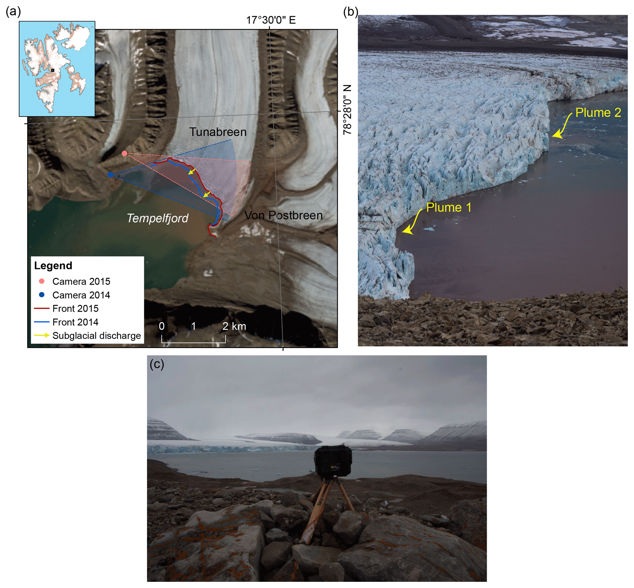
Figure 1 (a) Map of Tunabreen, Svalbard, with subglacial discharge positions, time-lapse camera positions and angles of vision. Front position as of September 2014 and August 2015. The satellite image is a Landsat 8 OLI–TIRS C1 Level 1 (14 August 2015). (b) Picture taken on 8 August at 15:00 showing the two plumes of Tunabreen. (c) Time-lapse camera used for 2014 analysis standing in front of Tunabreen.

Time-lapse cameras are convenient monitoring tools that have been used for different purposes in glaciology such as daily digital elevation models (James et al., 2014), propagation of flexion zones up-glacier (Murray et al., 2015), glacier velocities (Ahn and Box, 2010; Messerli and Grinsted, 2015; James et al., 2016), monitoring of supraglacial lake levels (Danielson and Sharp, 2013), and meltwater plume surface area (How et al., 2017) or glacier surges (Kristensen and Benn, 2012). Time-lapse imagery has also been used to quantify calving events manually, with different resolutions and different scaling methods, for Columbia Glacier, Alaska (Walter et al., 2010), Paierlbreen, Svalbard (Åström et al., 2014), Tunabreen, Svalbard (Åström et al., 2014; Westrin, 2015) and Rink Isbræ, West Greenland (Medrzycka et al., 2016). Alternative approaches have also been used to estimate the size and frequency of calving events at tidewater termini such as direct visual detection (e.g. O'Neel et al., 2007; Bartholomaus et al., 2012; Chapuis and Tetzlaff, 2014), icequake detection (e.g. Bartholomaus et al., 2012; Köhler et al., 2016) or satellite imagery (e.g. Schild and Hamilton, 2013).

To manually detect calving events from time-lapse cameras is a very laborious task that requires days of work and becomes too difficult when the number of images is too large. For example, if the manual processing of an image takes 2 min, the operator would need 17 days (8 h of work per day) to process a month of images with 10 min intervals. As a consequence, few studies use the potential of time-lapse cameras and do not analyse more than a few days. Automatic methods have the advantage of enabling longer time series but, to date, no satisfying automatic calving detection from time-lapse cameras has been developed.

Here, we utilize a method first presented by Adinugroho (2015) and Adinugroho et al. (2015) to automatically detect calving events from sequential time-lapse imagery. The algorithm follows five main steps in order to achieve this: image registration, segmentation of the calving front, change detection, mask reconstruction and size calculation. The results from this automatic method are compared to a manual detection of calving events to verify and evaluate its accuracy. We use observations from two time-lapse cameras placed at two different locations in front of a tidewater glacier in Svalbard, Tunabreen, during two consecutive summers, 2014 and 2015. The calving event locations at the front are compared to the position of two rising plumes observed at the front, and the distribution of event sizes is compared to a power-law curve.

2 Study area

Tunabreen is a 27 km long surging tidewater glacier draining from the Lomonosovfonna ice cap and terminating at the head of Tempelfjorden in central Svalbard (see Fig. 1). Its drainage area is approximately 174 km² (Nuth et al., 2013). This glacier is known to have surged in 1930, 1970 and more recently in 2002–2005, experiencing multiple retreats and advances and leaving submarine footprints (Forwick et al., 2010; Flink et al., 2015). It was retreating from its maximum extent, reached in 2004, until 2016 when it started to surge again. The 3 km wide terminus is roughly 70 m thick and grounded in 40 m deep water (Flink et al., 2015). At the front of Tunabreen, there is one main subglacial drainage portal (see Fig. 1) that can also be seen in the pictures (see Figs. 10 and 1b). The main subglacial plume, plume 1, is described in detail in Schild et al. (2017). A second subglacial plume, plume 2, is less visible and intermittently present in the pictures (see Fig. 1b). There are also two terrestrial melt streams, one on each side of the glacier.

3 Methods

3.1 Time-lapse cameras

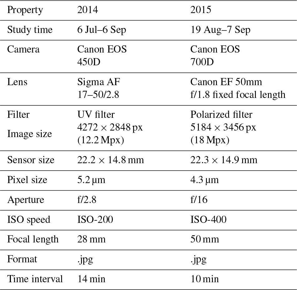
In 2014, a time-lapse camera was installed in front of the Tunabreen calving front, in the moraine field, at the coordinates (N78^∘ 27.084^′ E17^∘ 16.195^′ 73 m) shown in Fig. 1. The camera (Canon EOS 450D) was placed on a tripod in a waterproof plastic box (Pelican Storm IM2075) with a drilled hole in front of the camera (see Fig. 1). The intervalometer is a Digisnap 2700 from Harbortronics with a low temperature modification. The system was powered by a 12 V alkaline battery pack, placed in a plastic box covered by stones. The time interval between pictures was 14 min.

In 2015, an additional time-lapse camera was installed on Ultunafjella, a rock outcrop to the west of the glacier terminus. The camera (Canon EOS 700D) was enclosed in a custom-made Peli Case box along with a Harbortronics Digisnap 2700 intervalometer. This system was powered by an external 12 V battery and a 10 W solar panel. The camera system was installed on a tripod, and the tripod was buried into the ground and anchored by rocks.

In both years, the cameras were set in aperture priority (set aperture value and automatic shutter speed). The camera properties are presented in Table 1.

Table 1 Time-lapse camera properties for 2014 and 2015.

3.2 Image registration

Image registration is the process of transforming all images (or at least a sequence of images) into one coordinate system, enabling the comparison between these images. Detecting changes in a sequence of images requires perfect alignment of the images so that non-moving objects are at the same location for every image in the sequence. However, that condition may not hold in our case. Due to weather conditions, the camera can slightly move and rotate. This may cause false change detection if the images are not geometrically aligned. Thus, image registration is an important step in calving event detection.

Feature-based image registration makes use of shared features on a referenced image and a captured image in order to geometrically align the captured image to the referenced one. Speeded-up robust feature (SURF) descriptors (Bay et al., 2008) are extracted from both images. The descriptors from the two images are matched in order to select descriptors found in both images.

Geometric transformation occurring in two consecutive images can be revealed from a relation between matching descriptors in those images. The M-estimator SAmple Consensus (MSAC) algorithm (Torr and Zisserman, 2000) estimates affine transformation from descriptors so that the descriptors from the referenced image match most closely with those of the captured image. Based on this transformation model, the captured image can be transformed to geometrically match the reference image.

In Adinugroho et al. (2015), we registered all images to the first one, but this did not produce a good result when the image to register was separated by a long time because the glacier moves and the features in the ocean change. We thus choose to register each image to the previous one. However, when visibility is poor, matching features are scarce and this method does not perform well, so we use the registration characteristics of the former image. For the next image, if the visibility is better, we compare with the last good image. We estimate the registration process to perform well above 200 matching features (a normal image counts approximately 2000 features).

3.3 Automatic detection

3.3.1 Segmentation

The first step in the automatic detection of calving events is to isolate the calving front from the surroundings to avoid the detection of changes at the surface of the glacier or the ocean. First, the image is cropped around the glacier front geometry so that most noise is removed. The cropping region is determined from the first image. Second, we use a region-based active contour method, the Chan–Vese model (Chan and Vese, 2001), to isolate the front and the ocean.

The Chan–Vese model uses a region-based active contour, which works based on region information instead of edge information (boundary detection) as used by an edge-based active contour. We adopt the Chan–Vese model because it does not rely heavily on edge detection, which is often hard to find between the surface and the front of the glacier. It uses an evolving curve to detect objects in a given image u₀. To do that, the Chan–Vese segmentation minimizes an energy function defined as

$$\begin{array}{ll}{\displaystyle }F(c_{\mathrm{1}},c_{\mathrm{2}},C)=& {\displaystyle }\mathit{\mu }\cdot \mathrm{Length}\left(C\right)+\mathit{\nu }\cdot \mathrm{Area}\left(\mathrm{inside}\right(C\left)\right)\\ {\displaystyle }& {\displaystyle }+{\mathit{\lambda }}_{\mathrm{1}}\underset{\mathrm{inside}\left(C\right)}{\int }{\left|u_{\mathrm{0}}(x,y)-c_{\mathrm{1}}\right|}^{\mathrm{2}}\mathrm{d}x\mathrm{d}y\\ \text{(1)}& {\displaystyle }& {\displaystyle }+{\mathit{\lambda }}_{\mathrm{2}}\underset{\mathrm{outside}\left(C\right)}{\int }{\left|u_{\mathrm{0}}(x,y)-c_{\mathrm{2}}\right|}^{\mathrm{2}}\mathrm{d}x\mathrm{d}y,\end{array}$$

where μ, ν, λ₁ and λ₂ are non-negative parameters, and C is a curve that separates the image into two regions. c₁ and c₂ denote the mean intensity values of the two regions inside C and outside C, respectively. Equation (1) reaches its minimum if and only if the curve C lies at the boundary of two homogeneous areas.

At the first iteration, the user is required to delineate two initial masks, around the ocean, $M_{\mathrm{0}}^{\mathrm{ocean}}$, and the front, $M_{\mathrm{0}}^{\mathrm{front}}$, that are iteratively refined using the Chan–Vese model. In order to reduce computation time, the maximum number of iterations is limited to 50. We want to keep the pixels from the front mask but remove those from the ocean mask. At iteration i, the previous masks, $M_{i-\mathrm{1}}^{\mathrm{ocean}}$ and $M_{i-\mathrm{1}}^{\mathrm{front}}$, are used as initial masks of the Chan–Vese model to produce $M_i^{\mathrm{front}}$. Similarly to the registration process, if the visibility is bad we use the mask from the previous iteration.

3.3.2 Change detection

The goal is to detect changes between two grayscale images masked by the intersection of $M_{i-\mathrm{1}}^{\mathrm{front}}$ and $M_i^{\mathrm{front}}$. Because luminosity or weather conditions can have an impact on the change detection, pixel-based change detection methods are not adequate for this study. Instead, a region-based change detection method significantly reduces noise by computing the change in a pixel with respect to its neighbours and thus relying on local structural features (Li and Leung, 2002).

The rotationally dependent local binary pattern (LBP) is a simple visual descriptor method to extract the image texture T_i of image i (Ojala et al., 1996, 2002; Pietikäinen et al., 2011). The centre pixel, (x_c,y_c), in grayscale value, g_c, is compared to its P neighbour values situated at a radius R of coordinates $\left\{(x_{\mathrm{c}}+R\cos (\mathrm{2}\mathit{\pi }p/P),y_{\mathrm{c}}+R\sin (\mathrm{2}\mathit{\pi }p/P\left)\right),p\in [\mathrm{0},P-\mathrm{1}]\right\}$. The grayscale value, g_p, is linearly interpolated if not falling at the centre of a pixel. The texture value of the centre pixel (x_c,y_c) is then defined as

$$\begin{array}{}\text{(2)}& T_i(x_{\mathrm{c}},y_{\mathrm{c}})=\sum _{p=\mathrm{0}}^{P-\mathrm{1}}{\mathrm{2}}^p\mathit{\delta }(g_{\mathrm{p}}-g_{\mathrm{c}}),\end{array}$$

with δ(x) the Heaviside step function, which gives 0 if x<0 and 1 if x≥0. Here we use P=20 and R=5 for 2014 and R=6 for 2015. The different values depend on the characteristics of the camera (focal length, distance to the front, resolution, etc.), and the choice is empirical. Parameters P and R have been sampled in $[\mathrm{8},\mathrm{10},\mathrm{15},\mathrm{20},\mathrm{30},\mathrm{40}]$ and $[\mathrm{5},\mathrm{10},\mathrm{15}]$, respectively. The quality of the settings has been assessed by comparing errors between the automatic and the manual methods using the comparison metric presented in Sect. 3.5. For both years, the best results were achieved with P=20 disregarding the value of R. The value of the radius R is sensitive to the size of the image pixel.

To determine the amount of change in the texture of two consecutive images, we use the combined difference image and K-means clustering (CDI-K) as proposed by Zheng et al. (2014). Two operators, the absolute difference and the logarithmic difference, are applied to the texture images, T_i−1 and T_i, and produce two change images, D_s and D_t, respectively.

$$\begin{array}{}\text{(3)}& {\displaystyle }& {\displaystyle }{D}_{\mathrm{s}}=|T_{i-\mathrm{1}}-T_i|,\text{(4)}& {\displaystyle }& {\displaystyle }{D}_{\mathrm{t}}=\left|\log \right(T_{i-\mathrm{1}})-\log (T_i\left)\right|\end{array}$$

The change images are normalized to the range [0,255]. We then apply a mean filter (11×11) to D_s in order to remove isolated pixels and a median filter (3×3) to D_t in order to remove isolated pixels but preserve edges. The resulting images, $D_{\mathrm{s}}^{\prime }$ and $D_{\mathrm{t}}^{\prime }$, are combined, with the former achieving sleekness and the latter maintaining edge information, using a weight parameter w>0.

$$\begin{array}{}\text{(5)}& D=w{D}_{\mathrm{s}}^{\prime }+(\mathrm{1}-w)D_{\mathrm{t}}^{\prime }\end{array}$$

We set the weight parameter w=0.1 as suggested by Zheng et al. (2014).

To decide if there is change or no change, we choose to use a local neighbour threshold because of its deterministic nature in contrast with the randomness of K-means. A median function is applied to D on a 25×25 pixel window.

Figure 2 (a) Clustered points at which change has been detected using the method described in Sect. 3.3.2. (b) Mask reconstruction using the method described in Sect. 3.3.3, which transforms the clustered points into polygons.

When the weather is too foggy in one image, the whole calving front is detected as calved and it takes a long time for the algorithm to perform. We therefore remove images that fall into this category by calculating the coefficient of variation (CV) of the calving front, which gives an idea of the intensity distribution of the image. If the CV is above or below a certain threshold, determined beforehand from a set of images, the image is removed. The threshold has been determined by comparing errors between manual and automatic methods using the comparison metric presented in Sect. 3.5. Above the threshold, the image is highly illuminated, and below the threshold, the image is covered by dense fog. The front is almost not recognisable, so calculation is impossible and errors are systematically very large; the size of the automatically detected calving events is close to the size of the front.

3.3.3 Change mask reconstruction

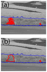
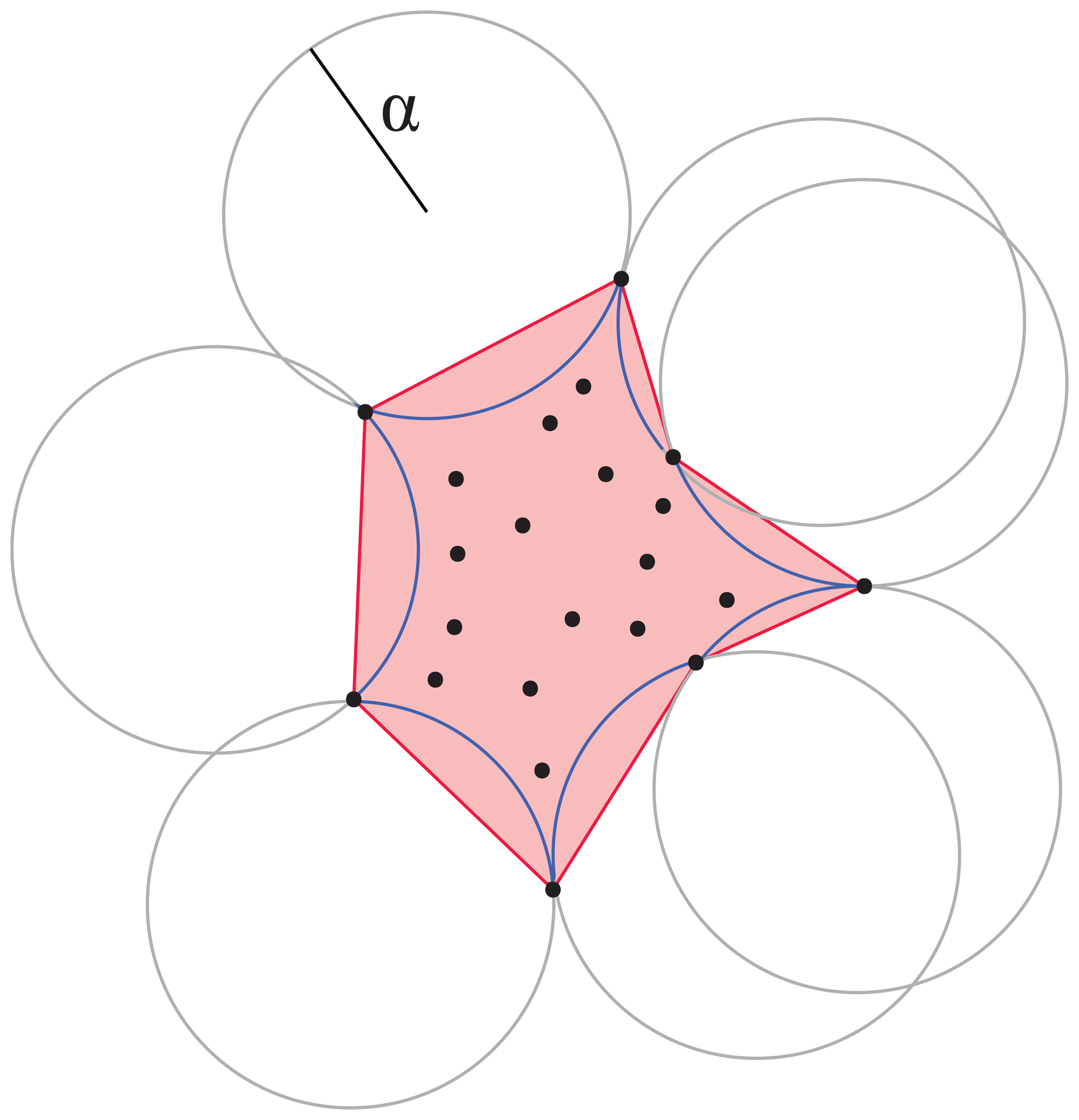
The end product of the change detection method detailed above is generally a set of clustered points of change (see Fig. 2a) and we use a mask reconstruction method, called the α-shape method (Edelsbrunner et al., 1983), to transform the result into polygons (see Fig. 2b). We can determine the set of points situated on the boundary of any empty open disc of radius α (the points situated on the blue curve in Fig. 3). The polygon is then constructed from these points (in red in Fig. 3). α is a very sensitive parameter and has to be chosen with care. If α tends towards zero, only the points themselves are kept. The smaller the value of α, the smaller the empty open discs around the points and the smaller the α shape (the reconstructed area). If α tends towards infinity, the α shape is the convex hull of the points. We further test the sensitivity of the mask reconstruction parameter α.

Figure 3 Schematic of the mask reconstruction using the α-shape method.

A polygon is kept if the number of pixels it contains is higher than a threshold; otherwise, it is considered noise. The size threshold depends on the real size of the pixels (described in the next section). To simplify, we use the real size of a pixel averaged over the whole front and a threshold of 50 m².

3.4 Size calculation

To estimate the pixel size we use the photogrammetric concept that the real pixel size is dependent on the focal length of the camera, the distance from camera to the front and the physical size of the pixel at the sensor. The distance to the front is calculated from georeferenced satellite images Landsat 8 OLI–TIRS C1 Level 1 downloaded from USGS EROS (10 images from July–September 2014 and 1 image from August 2015).

The front is outlined with a user-control tool in the image so we can determine the distance of the front in pixels, d. We outline the front on the satellite image and project it into the camera horizontal direction (black line in Fig. 4a) to get a number of d evenly distributed points. When projected back to the front (red line in Fig. 4a), the distance between each point (X_i,Y_i) is the real pixel size in the horizontal direction.

The real pixel area of the image pixel (x_i,y_i) is $A_i=d_X^i\times d_Z^i$, where $d_X^i$ and $d_Z^i$ are the real lengths of the pixel in the horizontal and vertical directions of the image, respectively (see Fig. 4). We need to determine the size of the projected pixel on the front in the horizontal direction, $d_X^i$, which depends on the orientation of the front, and the size in the vertical direction, $d_Z^i$, which depends on the camera position height, assuming that the front is vertical. To perform the projection we use reference points on the front, camera position (X_cam,Y_cam) and the focal angle $\mathit{\theta }=\mathrm{2}\arctan (x_{\mathrm{s}}/(\mathrm{2}{l}_{\mathrm{f}}\left)\right)$, where x_s is the sensor size in the horizontal direction and l_f is the focal length (see Table 1). In the vertical direction, we assume a vertical front and calculate the distance, L_i, from the camera to the front. We assume no distortion of the projected pixels in the vertical direction so that each pixel on a vertical column has the same size (same distance from the camera), and we correct for the elevation, Z_cam, of the camera location. The real size of the pixel in the vertical direction, $d_Z^i$, is then

$$\begin{array}{}\text{(6)}& d_Z^i={\displaystyle \frac{L_i}{l_{\mathrm{f}}}}{y}_{\mathrm{px}},\end{array}$$

where $L_i=\left(\right(X_{\mathrm{cam}}-X_i{)}^{\mathrm{2}}+(Y_{\mathrm{cam}}-Y_i{)}^{\mathrm{2}}+Z_{\mathrm{cam}}^{\mathrm{2}}{)}^{\mathrm{1}/\mathrm{2}}$ is the distance from the camera to the front at sea level and y_px is the image size of a pixel in the y direction. Calibration is an important step, particularly when working with sizing, that permits us to retrieve intrinsic parameters of the camera. This work was done in 2015 but not in 2014 and should be systematically used in the future. Lens distortions are neglected here. The radial distortion relative error for the front pixel situated the farthest from the camera is around 0.6 % for 2014 and 0.15 % for 2015. To calculate these figures, we used the Barrel distortion correction given a set of coefficients $(a,b,c)$ such as $r_{\mathrm{d}}=a\cdot r_{\mathrm{u}}^{\mathrm{4}}+b\cdot r_{\mathrm{u}}^{\mathrm{3}}+c\cdot r_{\mathrm{u}}^{\mathrm{2}}+d\cdot r$, with $d=\mathrm{1}-(a+b+c)$, r_d and r_u the distorted and undistorted distance from the focal centre to the pixel. The coefficients have been taken from a camera database (Bronger, 2018).

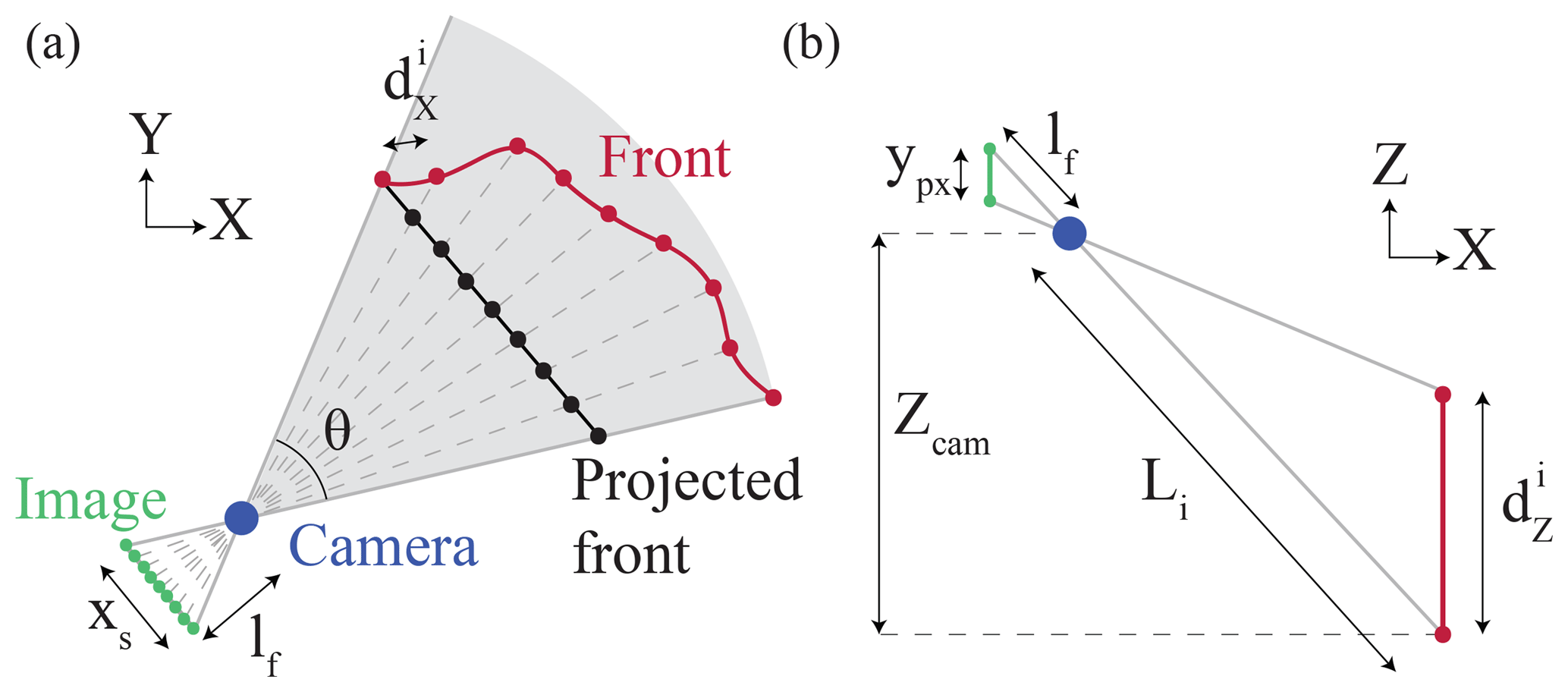
Figure 4 Schematic of the size calculation (a) in the horizontal direction and (b) in the vertical direction.

3.5 Comparison with manual method

In order to assess the performance of the automatic detection method, we compare the results to a manual method on the same set of images using human visual detection. This does not give the absolute accuracy of the method in relation to true calving since this would require an independent dataset. In 2014, 1100 images were used for comparison of automatic detection for the period 26 August to 6 September. In 2015, 469 images were used for the period 1 to 4 September.

3.5.1 Visual detection

Visual detection of calving events is performed by comparing two consecutive images. It is possible to zoom to a certain section of the glacier and switch from one picture to another to visually detect a change in the glacier front texture. A detected change, which represents a calving event, is outlined manually and the coordinates are saved. The manual detection for 2014 was performed by Westrin (2015).

Figure 5 Weather conditions and illumination categories: (a) normal (N), (b) light fog (LF), (c) dense fog, (d) high illumination and (e) low illumination.

3.5.2 Comparison metrics

The location and size of each calving event are the main results we want to retrieve. For the location, we construct a confusion matrix, which gives the agreements and disagreements between the automatic and the visual detection for each pair of masked images (e.g. Stehman, 1997) and which contains the following.

• A true positive (TP) is the number of pixels labelled as calved in both detections.

• A false positive (FP) is the number of pixels labelled as calved in the automatic detection but not in the visual detection.

• A true negative (TN) is the number of pixels labelled as non-calved in both detections.

• A false negative (FN) is the number of pixels labelled as calved in the visual detection but not in the automatic detection.

The number of pixels automatically detected as calved and non-calved are $P_{\mathrm{auto}}=\mathrm{TP}+\mathrm{FP}$ and $N_{\mathrm{auto}}=\mathrm{TN}+\mathrm{FN}$, respectively. The number of pixels visually detected as calved and non-calved are $P_{\mathrm{visual}}=\mathrm{TP}+\mathrm{FN}$ and $N_{\mathrm{visual}}=\mathrm{TN}+\mathrm{FP}$. The total number of pixels is $m=\mathrm{TP}+\mathrm{FP}+\mathrm{TN}+\mathrm{FN}$. It is important to note that, for the case of glaciers such as Tunabreen with a limited calving event size, the number of pixels labelled as calved is generally small compared to non-calved pixels. In this sense, the accuracy measure $\mathrm{Acc}=(\mathrm{TP}+\mathrm{TN})/m$ is not appropriate since TP≪TN as stated by Kubat et al. (1998) for imbalance classes. Here we need a method to detect changed regions, instead of unchanged ones. They recommend the use of the F measure to detect a classification problem with imbalanced classes. However, the F measure has a property that is invariant under the change in TN (Kubat et al., 1998), and thus it is less sensitive to changes in unchanged pixels. Alternatively, the Matthews correlation coefficient (Matthews, 1975),

$$\begin{array}{}\text{(7)}& \mathrm{Mcc}={\displaystyle \frac{\mathrm{TP}\times \mathrm{TN}-\mathrm{FP}\times \mathrm{FN}}{\sqrt{P_{\mathrm{auto}}\times P_{\mathrm{visual}}\times N_{\mathrm{visual}}\times N_{\mathrm{auto}}}}},\end{array}$$

is a better measure for imbalanced classes and it takes into account both true and false positives. Its interpretation is similar to the Pearson correlation coefficient between the observed and predicted binary classifications. A value of +1 represents a perfect match, while −1 represents total disagreement. A perfect match only happens when no change is detected by both methods. When there is no overlap or a calving event is only detected by one of the methods, the Mcc will give a low value by definition, whatever the size of the detected event. To be able to compare the magnitude of the error, we can look at the positive difference as the difference between detected calved zones from both methods divided by the total number of pixels,

$$\begin{array}{}\text{(8)}& P_{\mathrm{diff}}={\displaystyle \frac{P_{\mathrm{auto}}-P_{\mathrm{visual}}}{m}},\end{array}$$

to assess the importance of the mismatch.

Weather conditions and illumination change the pixel intensities and can inhibit detection in some cases. We determined five categories: normal conditions (N), light fog (LF), dense fog (DF), high illumination (HI) and low illumination (LI). Some examples are shown in Fig. 5. When comparing manual and automatic detection, we visually determine the categories qualitatively. Each image has also been cut in six different sections placed in a weather condition category.

4 Results

4.1 Comparison assessment

An example of calving detection from the automatic and manual methods is shown in Fig. 6.

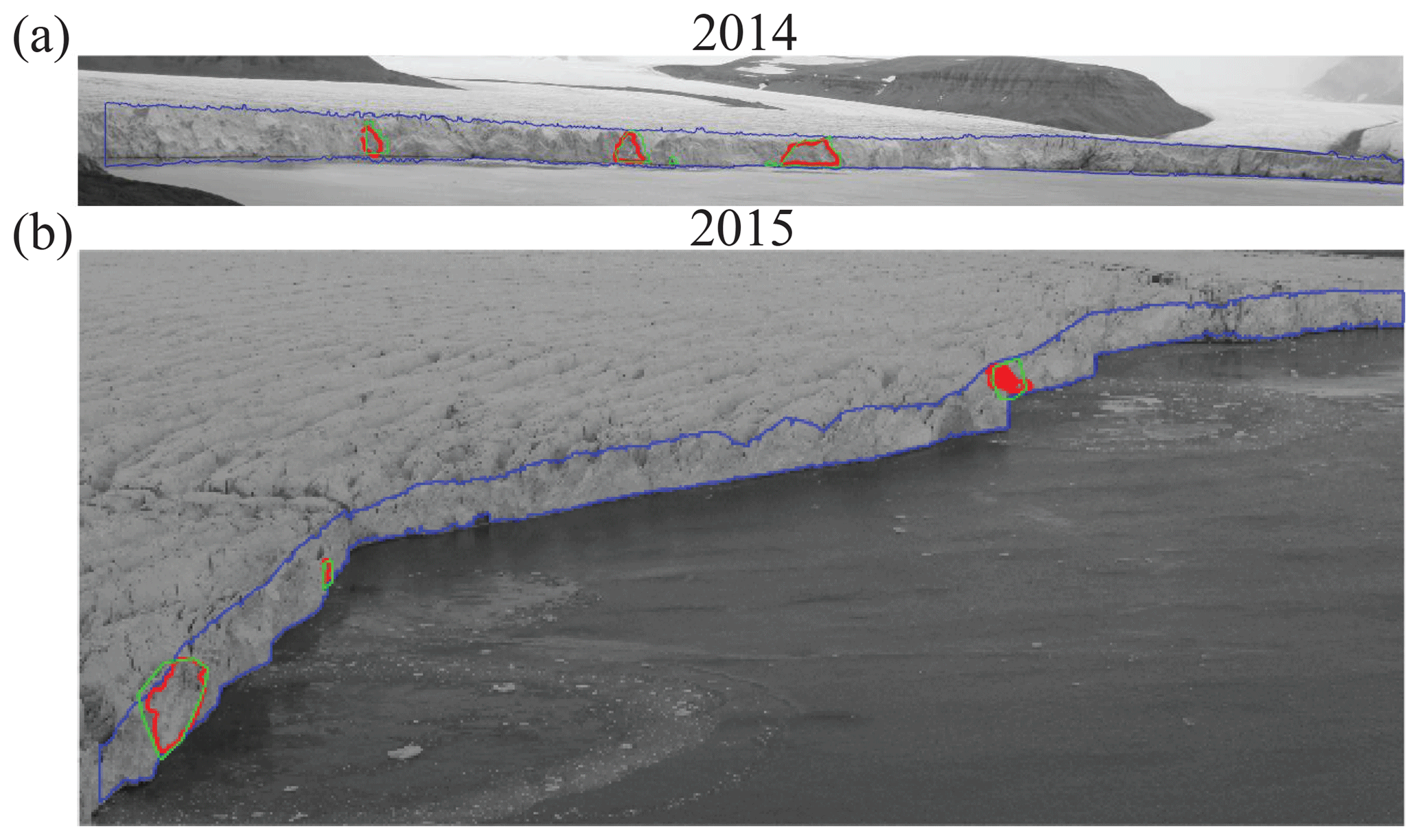
Figure 6 Example of mask delineation (blue), automatic calving detection (red) and manual calving detection (green) for (a) 2014 (2 September, 11:45) and (b) 2015 (1 September, 19:21).

Different weather conditions have been studied at six different sections of the glacier (see Fig. 10), and the Mcc and P_diff are shown in Fig. 7 for 2014 (a) and 2015 (b). We chose not to show the perfect match Mcc=1, corresponding to no detection of calving, for both methods in the figure because a fairly large number of images do not have calving and it skews the results towards 1. Instead, we chose to show the percentage of occurrences for which Mcc=1 in Table 2. To assess the errors, we use the Mcc when there are matching pixels for both detections (Mcc≠0) and P_diff otherwise (Mcc=0). In general, normal conditions (N), light fog (LF), low illumination (LI) or a combination of these conditions have a high Mcc, with a mean close to 0.7 (2014) or 0.5 (2015), and can be considered good matches. When Mcc=0, the difference between pixels, P_diff, is close to zero. In contrast, dense fog (DF), high illumination (HI) and any combination with one or the other show a relatively low Mcc and particularly high P_diff. If such a configuration is combined with any of the others, the result is also poor.

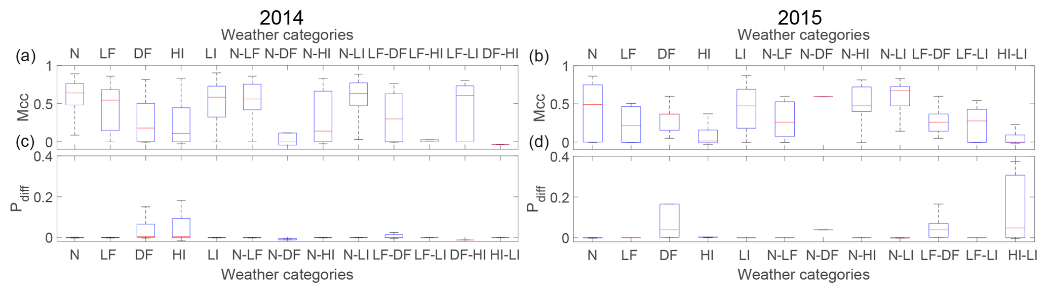
Figure 7 Box plot of Matthews correlation coefficient, Mcc, when Mcc≠0 and Mcc≠1 for (a) 2014 and (b) 2015. Positive difference percentage, P_diff, when Mcc=0 (no matched pixel) for normal conditions (N), light fog (LF), dense fog (DF), high illumination (HI), low illumination (LI) and a combination of each for (c) 2014 and (d) 2015.

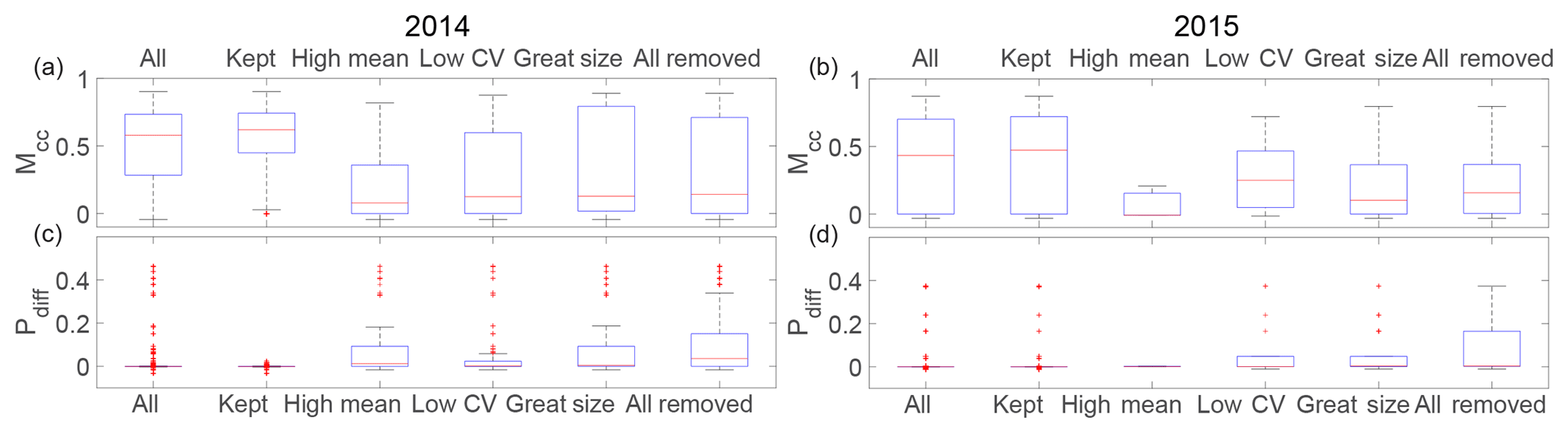
Figure 8 (a) Box plot of Matthews correlation coefficient, Mcc, when Mcc≠0 and Mcc≠1 and (b) positive difference percentage, P_diff, when Mcc=0 (no matched pixel) for all images, for the images kept, and for the images removed from the high-intensity mean, low-intensity coefficient of variation (CV) or size thresholds.

Table 2 Percentage of Mcc=1 for each weather category.

We decided to remove all pictures with high illumination and dense fog from the analysis. To determine whether a picture falls into this category, we look at the standard deviation and mean of pixel intensity for each section of the image after calibrating these values for different lightning conditions on a set of images. Pictures with a high mean intensity compared to the normal range for each section fall into the high illumination category. Pictures with low CV (ratio between standard deviation and mean intensity) fall into the dense fog category. Moreover, given the calving characteristics of Tunabreen (generally no glacier-wide calving events), we assume that if the detected calving size is greater than a certain value depending on the front size, the detection is not satisfactory and we thus remove it from the results. Fig. 8 shows the results for 2014 and 2015. This method has limitations since even if it performs well at removing bad detection, it also removes good ones.

To test the sensitivity of the mask reconstruction parameter α, we look at five different values and compare the results after removing unfavourable weather. This is shown in Fig. 9. If α is too small, the event sizes from the automatic detection tend to be smaller than from the manual detection and vice versa for too-big α. In Fig. 9, the best fit between manually and automatically detected calving events is when α=10 given the Mcc and P_diff results.

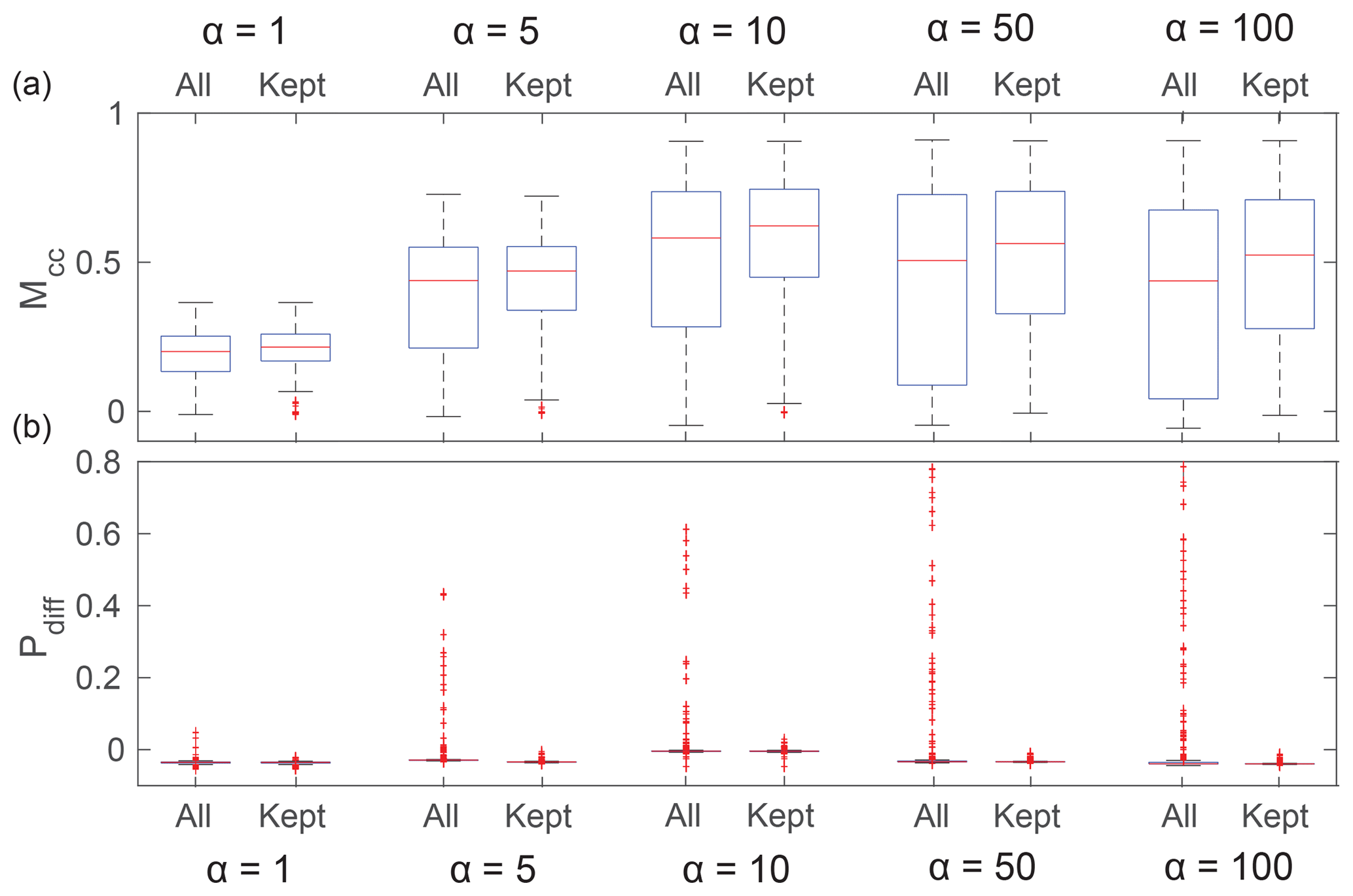
Figure 9 (a) Box plot of Matthews correlation coefficient, Mcc, when Mcc≠0 and Mcc≠1 and (b) positive difference percentage, P_diff, when Mcc=0 (no matched pixel) for all images and for the images kept given different values of the mask reconstruction parameter α.

4.2 Calving detection

The initial number of pictures to be analysed in 2014 was 6292, but because of weather conditions and camera settings, only 3497 usable images remain, of which 2084 showed no calving. In total, 2575 calving events have been detected, ranging from 20 to 3500 m². An example of mask delineation and calving detection is given in Fig. 10a. To facilitate the analysis, the front is divided into six sections as shown in Fig. 10a. The number of calving events detected in each section is 524 in section 1, 681 in section 2, 455 in section 3, 341 in section 4, 344 in section 5 and 230 in section 6.

In 2015, 3242 images were analysed, but 571 of these were removed as the glacier terminus was obscured by water droplets on the porthole cover of the time-lapse enclosure. Because of this, there is no coverage for 23–27 August. After weather filtering, 1495 images are left, including 898 with no calving detection. In total, 1647 events were detected (222 in section 1, 327 in section 2, 228 in section 3, 234 in section 4, 398 in section 5 and 238 in section 6). An example of mask delineation and calving detection is given in Fig. 10b.

Figure 10 Example of mask delineation (blue) and calving detection (red) for (a) 2014 (4 September, 16:01) and (b) 2015 (19 August, 19:10). The front is divided into six sections shown in the figure.

4.3 Spatio-temporal size distribution

In Fig. 11, we present the total area detected per image (in blue) and the daily moving average (in red). It is difficult to establish a seasonal pattern because of the data gaps during unfavourable weather conditions.

Instead, we explore the relative size distribution for the different sections to estimate which section undergoes the largest calving events per image (see Fig. 12a–c). When calving events are detected in an image, we look at the size proportion of each section. If, for a pair of images, calving is detected in only one section, this section gets 100 % of the total. If other events occur within the same time frame in other sections, these sections get a proportional fraction corresponding to their size compared with the total calved size of the whole calving front. The primary event section receives the largest share. In Fig. 12b–d, for each primary event section, we show the share of the secondary event.

If a section gets 100 % of the total size during a time frame, it is more often section 2, followed by section 5 in 2014, whereas in 2015, it is more often section 5, followed by section 2. In general, section 2 for 2014 and section 5 for 2015 have the most occurrences of primary calving event size. Also, when a primary calving event size occurs in section 5, secondary calving occurs particularly in section 2. For 2015, section 5 is also secondary when section 2 is primary. It is also where the most margin retreat occurs in the season. Furthermore, there seems to be a link between sections. When a primary calving event occurs in a section, secondary calving event sizes are usually found in adjacent sections.

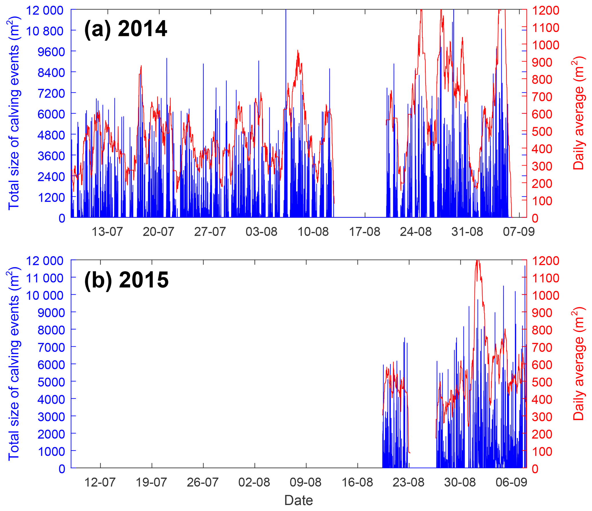
Figure 11 Total size detected per image (in m²) in blue and moving average on a daily basis (in m²) in red for (a) 2014 and (b) 2015.

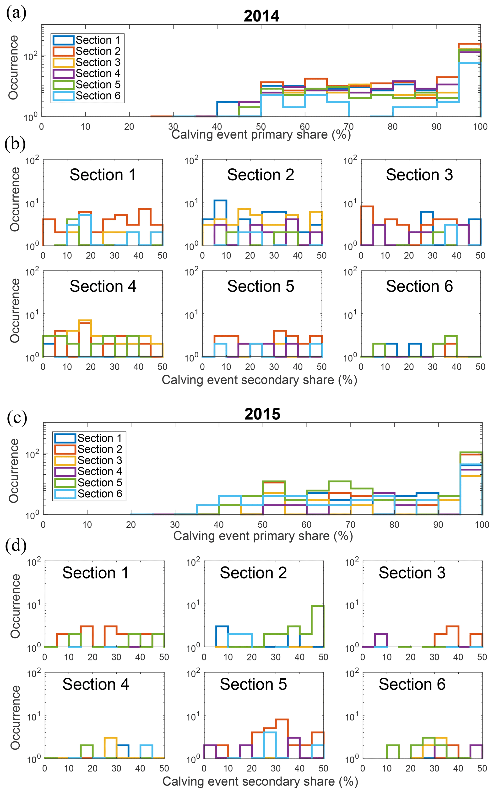
Figure 12 Size proportion histogram of the major calving event size per image for (a) 2014 and (c) 2015. Size proportion histogram of the secondary calving event size per image and per section for (b) 2014 and (d) 2015.

4.4 Event size distribution

Figure 13 shows the event size relative abundance distributions for both years. The relative abundance n(A) is the ratio between the frequency and the sample size of calving areas A. The plain curves are power-law estimates of exponent −1.2 for both years. There is a cut-off for large sizes around 5×10³ m².

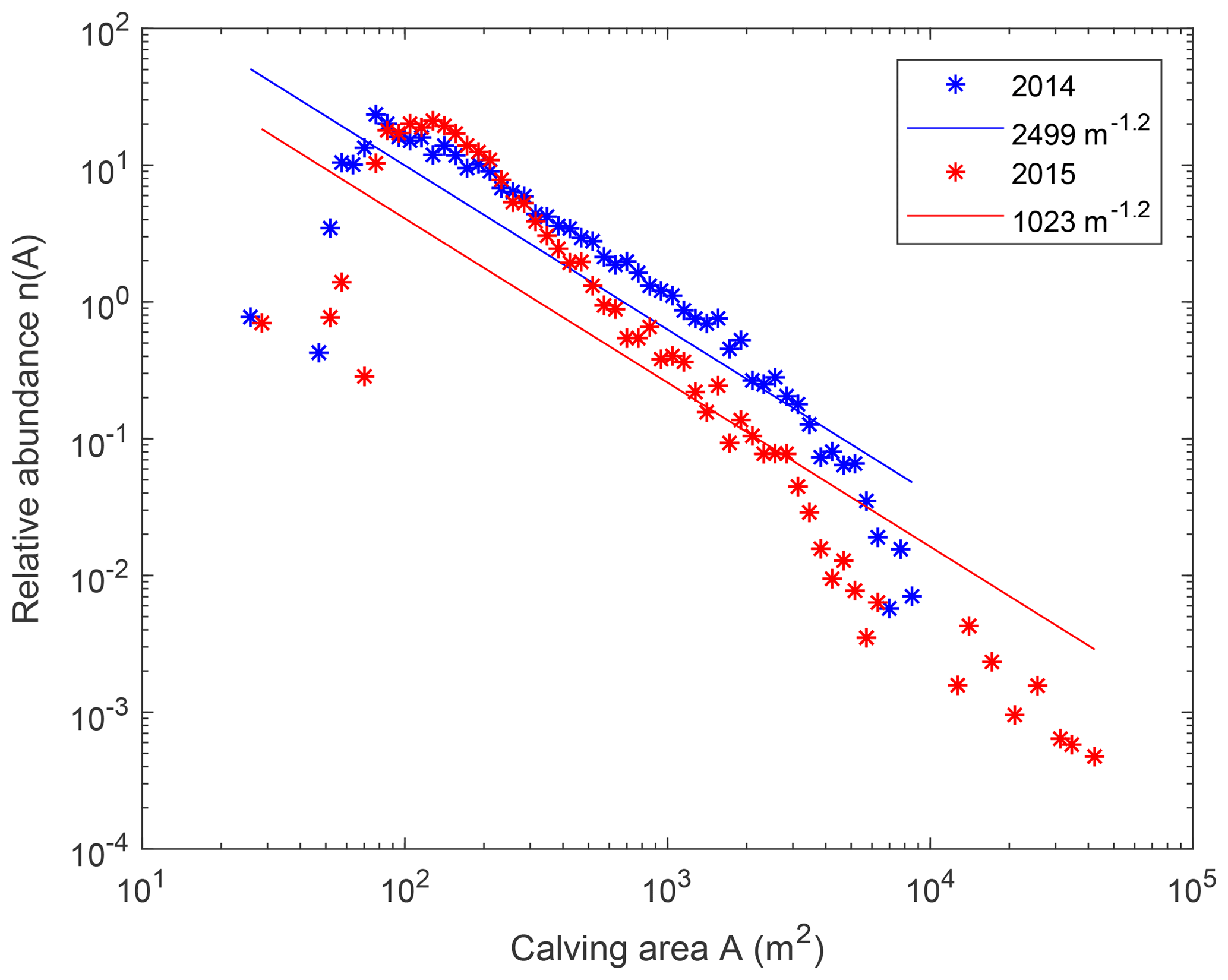
Figure 13 Relative abundance distribution n(A) of calving areas A for 2014 (blue stars) and 2015 (red stars). The plain curves are power-law estimates of exponent −1.2 for 2014 (blue) and 2015 (red).

5 Discussion and conclusion

5.1 Calving, plumes and self-organized criticality

The spatio-temporal information such a method provides has the potential to enhance understanding of certain processes or validate calving theories. Here we used two time series of two different years from two different locations and camera settings. Some problems still need to be addressed and are discussed in the following section. The long time lapse and weather-related issues do not allow for direct conclusions on the spatio-temporal calving behaviour of Tunabreen. Still, it appears that most of the large calving events happened near plume locations (sections 2 and 5) with larger events at the most active plume location, plume 1 (section 2). The plume in section 5 has not been detected elsewhere in the literature, so this conclusion has to be taken with care and should be investigated further. It also appears that when a large event is triggered at the less active plume location, plume 2 (section 5), a smaller one is simultaneously triggered at plume 1. Moreover, events in one section seem to trigger smaller events in adjacent sections, which confirms the destabilization of the local neighbourhood of the calving region observed by Chapuis and Tetzlaff (2014).

A self-organized critical (SOC) system in nature is a system that exhibits a slow and steady accumulation of an instability followed by a rapid relaxation triggered from a single point and, independently of external conditions, leading to a collapse of any possible size (Jensen, 1998). Åström et al. (2014) showed that the calving front behaviour of tidewater glaciers have the characteristics of an Abelian sandpile model, a simple SOC system (Dhar, 1999). The probability distribution at the critical point approaches a power law with an exponent close to −1.2, which is also the case for the results shown in Fig. 13. Cut-offs for large sizes have also been reported in Åström et al. (2014) for smaller glaciers, and they are due to the glacier front size. For smaller sizes, the relative abundance is below the power-law estimate. This is either due to the long time lapse between images, which does not allow small events to be detected, or to the spatial resolution of the camera. The correlation coefficient for 2014 is R²=0.12 including events smaller than 100 m² and R²=0.98 without. For 2015, R²=0.08 and R²=0.96, respectively. The system always tends towards criticality without regard to external factors. However, external conditions have the potential to change the system from subcritical to supercritical. An investigation of the relationship between calving events and environmental controls will be the subject of a separate paper.

5.2 Errors and limitations

The main limitation is clearly poor performances due to weather: in the presence of fog or when the calving terminus is strongly illuminated by the sun. The illumination problem is worst during daytime when the sun is reflected on the ice. At those times, mostly in the middle of the day, the temperature is high, leading to surface melt, subglacial discharge and active plume. The marine melt feedback is therefore difficult to analyse with this method if the weather condition problem is not solved. Nevertheless, in normal conditions or low illumination, the method performs well compared with the manual method and is a good tool to assess the location of calving events. Errors in detection, however, may arise because of different factors. First, the method requires different parameters at each step and most of them are defined empirically (trial and error), particularly the change detection and mask recognition parameters, but also the threshold for unfavourable weather conditions and minimum–maximum calving size. Second, the method detects frontal changes and is not able to recognize external objects coming into view of the camera, such as birds or icebergs, or detect the difference between frontal ice changing position because of gravity, for example, and actual calving. Third, while the glacier front calves, it also advances due to ice flow and both processes have an effect on the front position. Because of that, the front outline needs to be manually refined periodically, depending on the flow speed of the glacier and the camera view angle. For Tunabreen, refinement was needed every 1000 pictures or every 8–10 days. Fourth, no subaqueous calving can be detected with this method, although for certain glaciers this could account for a large proportion of the frontal mass loss. Finally, manual detection is subject to error because of a failure to correctly identify or digitize events.

5.3 Recommendations and future improvements

Despite inherent limitations, the method can still be improved. First, the camera settings and camera installation have an impact on the result and can be optimized. For the set-up in 2014, the large aperture setting (f/2.8) and the lack of a polarized filter rendered more pictures compared to 2015 falling into the HI category. It is important to consider all of the situations that the automatic settings of the camera will have to handle. Also, instead of fixing the aperture width, one could fix the aperture speed to let the lens adapt to the amount of light available or adapt the ISO, as in Kwasnitschka et al. (2016). The position of the camera also influences the results, and our two different camera locations show both benefits and drawbacks. A camera positioned at low elevation and in front of the glacier (2014) is favourable for segmentation (refinement has to be done less often), whereas a camera situated more to the side and at higher elevation (2015) is favourable for recognizing larger events, but parts of the front may be occluded. In some images, calving events are recorded at different locations, and having a shorter time-lapse interval (to be set according to the characteristics of the glacier) could help to distinguish single events. Storing the images in lossy file format (like .jpg) also certainly degrades the quality and the ability to record events. Depending on how often the memory card can be changed or if there is a service for automatically downloading images, it would help to store the pictures in raw format so that more post-processing is available.

Second, the method can be improved for detecting or enhancing images with unfavourable weather. Fog detection is implemented for different applications (e.g. automatic car navigation) and could be useful (e.g. Hautière et al., 2014). If weather observations are available, it can also be good to combine these data to detect the total white-out of an area, for example (Jiskoot et al., 2015).

Third, the size calculation only gives the two-dimensional area of the calving event, and a third dimension could be calibrated from observation (Chapuis and Tetzlaff, 2014) or from other cameras placed at different locations. Moreover, the distance between the camera and the front is estimated from satellite data with rather low spatio-temporal resolution, and data with higher resolution could improve the size calculation (e.g. satellite, other time-lapse cameras or unmanned aerial vehicle photogrammetry).

This automatic method has been developed for a particular glacier, Tunabreen, but can be calibrated for other glaciers, even if the spatio-temporal scale is different. For instance, glaciers in Greenland, where calved icebergs are larger and detached more often, are a good candidate. Time-lapse cameras are easy to place in front of a glacier to monitor the calving state, and this method can help to automate an otherwise difficult task.

Deep learning is a potential method to segment glacier front from other regions. However, we found some potential issue with that method. It is relatively easy to separate glacier front from other regions, such as rock, soil and water. But, separating the front from the top part of the glacier is not easy since both parts look similar both visually and texturally. An experiment with some classifiers to segment glacier front did not show satisfying results. All methods failed to separate glacier front and top, especially around the boundary of those regions. It would also require a powerful machine (and powerful graphic card) and resources. Nevertheless, the idea should not be abandoned and could be subject to further improvements. We could also imagine determining cases in which each method works best.