Dense point cloud acquisition with a low-cost Velodyne VLP-16

This study develops a low-cost terrestrial lidar system (TLS) for dense point cloud acquisition. Our system consists of a VLP-16 lidar scanner produced by Velodyne, which we have placed on a motorized rotating platform. This allows us to continuously change the direction and densify the scan. Axis correction is performed in post-processing to obtain accurate scans. The system has been compared indoors with a high-cost system, showing an average absolute difference of ±2.5 cm. Stability tests demonstrated an average distance of ±2 cm between repeated scans with our system. The system has been tested in abandoned mines with promising results. It has a very low price (approximately USD 4000) and opens the door to measuring risky sectors where instrument loss is high but information valuable.

1 Introduction

Over these last decades, remote sensing and associated technologies have been developed and used to greatly improve environmental modelling. In particular, light detection and ranging (hereafter lidar) has been proposed as a tool in geomatics to address such environmental modelling. Lidar technology is based on the time of flight (ToF, i.e. the time required by the light emitted by the laser to be reflected and captured again by the system) to measure distances. Lidar is useful for solving many problems. It is therefore widely used in geosciences, in particular for the management and the monitoring of environmental risks such as landslides, rock falls or cavity collapse (Lim et al., 2005; Teza et al., 2007; Jaboyedoff et al., 2011; Brideau et al., 2012; Royán et al., 2014; Michoud et al., 2015). The reliability of these measuring instruments is well established, but the technology is typically very expensive, which limits the potential applications of such systems.

New lidar-based obstacle avoidance technologies have been under development since the advent of autonomous cars. These mass-produced sensors are cheap but were not initially designed to produce dense point clouds and therefore have reduced ranges and resolutions. These low-cost systems have led to the development of new scanner systems that can be applied for mapping, especially for mobile terrestrial SLAM-based systems (James and Quinton, 2014; Dewez et al., 2017) or unmanned aerial vehicle (UAV) SLAM-based systems (Laurent et al., 2019; Li et al., 2014) and often require the addition of an inertial station and Global Navigation Satellite System (GNSS).

Instruments used in geodesy such as theodolites or total stations must be calibrated to avoid measurement errors. This principle is also applied to lidar, which is constructed in a similar way. Lidar system calibration is a much studied subject in research. The aim is to determine the parameters that allow systematic errors to be reduced as much as possible. According to Neitzel (2006), three major errors may be present: tilting axis error, collimation error and eccentricity of the line of sight. Some authors describe up to 21 possible calibration parameters (Lichti, 2007). There are different strategies for calibrating a lidar system. Research proposes a self-calibration based on mathematical models and by making geometric primitives reference planes (Glennie and Lichti, 2010; Lerma and Garcia-San-Miguel, 2014) or reference points (Neizel, 2006; Kersten et al., 2005). Other authors present calibration methods based on the use of a camera (Amiri Parian and Grün, 2005; Lichti et al., 2007).

Our study is based on the use of a low-cost lidar system, which is the VLP-16 of Velodyne, to elaborate on a low-cost terrestrial lidar system (TLS). This scanner, currently sold for USD 4000, has 16 parallel scan lines in a vertical field of view of ±15^∘ and a 360^∘ horizontal scan plane (Fig. 2c). Our idea was based on the addition of a rotating plate (which is a principle similar to that of many lidar systems) to produce a dense point cloud. Such a system particularly targets applications in rough field conditions, such as caves that are difficult to access. In such places there is the likelihood of damage to the equipment due to shocks, water or dirt, which prevents the use of high-cost equipment. This type of system could also facilitate risk management in mines for the development of cave collapse risk maps, for example. The advantage is that the system is inexpensive, making it particularly suitable for permanent laser scanning in hazardous areas as described in Williams et al. (2018). In addition, the power consumption of low-cost lidars is often very small, which is suitable for such environments.

The structure of this paper is as follows: Sect. 2 presents the equipment and the constraints associated with it to produce a low-cost system. Section 3 presents the methodology used to produce high-resolution scans. Section 4 presents the result of our system. Section 5 discusses the results and Sect. 6 presents some conclusions.

2 Low-cost hardware

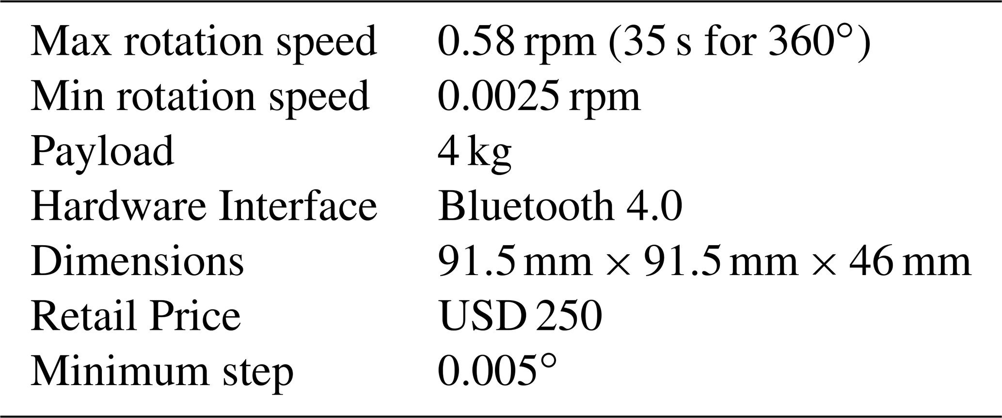
2.1 VLP-16 lidar

The VLP-16 model has 16 lasers fixed on a rotational head. The main features of the low-cost lidar can be found in Table 1.

Table 1 Velodyne VLP-16.

Each of the 16 parallel scan lines records up to 1875 points every tenth of a second, which corresponds to an angular horizontal resolution of 0.2^∘ for a field of view of 360^∘. Regarding the vertical resolution, the sensor is limited to a field of view of 30^∘ (Fig. 2c). The 16 scan lines imply a low vertical angular resolution of 2.0^∘. Each of the 16 lasers in VLP-16 is individually aimed and, thus, each has a unique set of adjustment parameters. The mathematical model of VLP-16 which calculates the (x, y, z) coordinates is given in Glennie and Lichti (2010) as

$$\begin{array}{rl}& \left[\begin{array}{c}x\\ y\\ z\end{array}\right]=\\ & \left[\begin{array}{c}(s^i\cdot R_i+D_{\mathrm{o}}^i)\cdot \text{cos}\left({\mathit{\delta }}_i\right)\cdot \left[\sin \left(\mathit{\epsilon }\right)\cdot \text{cos}\left({\mathit{\beta }}_i\right)-\text{cos}\left({\mathit{\epsilon }}_i\right)\right]\\ -H_{\mathrm{o}}^i\cdot \left[\text{cos}\left(\mathit{\epsilon }\right)\cdot \text{cos}\left({\mathit{\beta }}_i\right)+\sin \left(\mathit{\epsilon }\right)\cdot \sin \left({\mathit{\beta }}_i\right)\right]\\ (s^i\cdot R_i+D_{\mathrm{o}}^i)\cdot \text{cos}\left({\mathit{\delta }}_i\right)\cdot \left[\text{cos}\left(\mathit{\epsilon }\right)\cdot \text{cos}\left({\mathit{\beta }}_i\right)+\text{sin}\left({\mathit{\epsilon }}_i\right)\right]\\ +H_{\mathrm{o}}^i\cdot \left[\text{sin}\left(\mathit{\epsilon }\right)\cdot \text{cos}\left({\mathit{\beta }}_i\right)-\text{cos}\left(\mathit{\epsilon }\right)\cdot \text{sin}\left({\mathit{\beta }}_i\right)\right]\\ (s^i\cdot R_i+D_{\mathrm{o}}^i)\cdot \text{sin}\left({\mathit{\delta }}_i\right)+V_{\mathrm{o}}^i\end{array}\right],\end{array}$$

where sⁱ is the distance scale factor for laser i; $D_{\mathrm{o}}^i$ is the distance offset for laser i; δ_i is the vertical rotation correction for laser i; β_i is the horizontal rotation correction for laser i; $H_{\mathrm{o}}^i$ is the horizontal offset from scanner frame origin for laser i; $V_{\mathrm{o}}^i$ is the vertical offset from scanner frame origin for laser i; R_i is the raw distance measurement from laser i; and ε is the encoder angle measurement.

The first six parameters are used to calibrate the system and can be found in the lidar data sheet. R_i and ε come from data collected during a measurement.

Figure 1a shows a photograph of the scanned scene with the same viewing angle, and Fig. 1b shows a typical point cloud produced by the VLP-16 with highlighted vertical and horizontal angular resolutions. The poor vertical resolution limits the use of the VLP-16 for terrestrial scanning applications. For example, the low point density makes it difficult to co-register several scans.

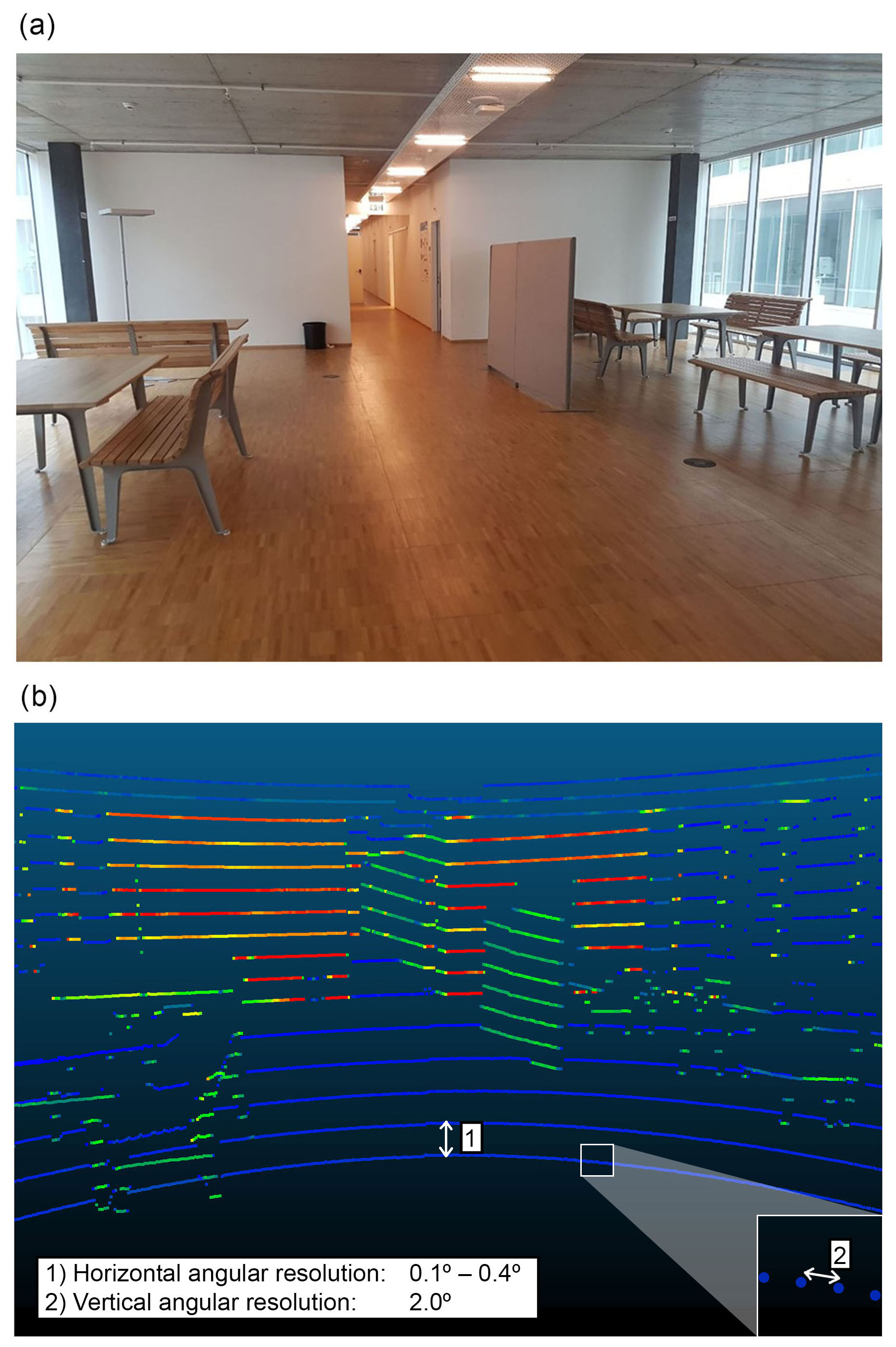
Figure 1 (a) Picture of the scanned scene; (b) a typical scan created with the VLP-16, the colour represents the intensity of the returned signal.

2.2 Syrp Genie

For the purpose of having a low-cost design, we select the Syrp Genie Mini (Table 2). This motorized head can rotate 360^∘ and sustain the weight of the lidar.

Table 2 Syrp Genie.

2.3 Conception and assembly of the custom scanning system

The VLP 16 is mounted on the Syrp Genie Mini, and the entire assembly is set on a photographic tripod and connected to a computer and a power source (Fig. 2a). Importantly, the lidar is placed vertically using an L-shaped piece, such that the vertical (low-resolution) and horizontal (high-resolution) directions are now reversed. It is also important to note that the term “vertical” corresponds to the lidar reference system and not necessarily to the direction of the gravitational field. Our goal is to use the slow rotating motion induced by the Syrp Genie Mini to densify the point cloud across the horizontal direction. It includes a stepper motor with a minimum step of 0.005^∘ which does not impact the acquisition frequency of the VLP-16. A counterweight is placed on the tripod on the opposite side of the lidar to minimize stresses that can impact the rotation speed and induce an angular distortion.

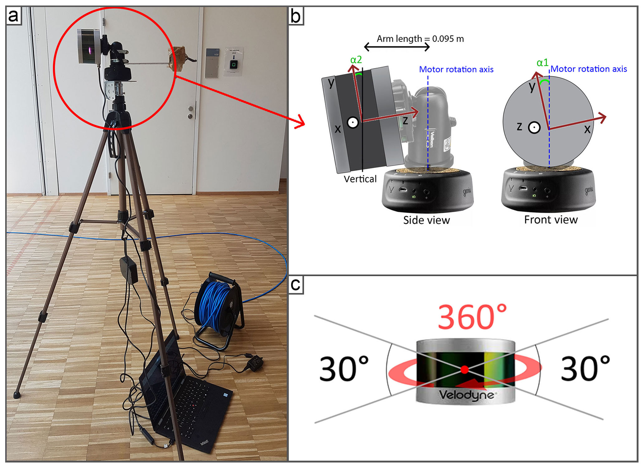
Figure 2 (a) Terrestrial lidar system (TLS); (b) two adjustments angles: collimation axis (α₁) and tilting axis (α₂) between the system and the rotation axis; (c) field of view of the VLP-16.

3 Methodology

3.1 Data acquisition operation

Acquisition with our system requires a number of post-processing steps to obtain a scan that correctly represents the scene. For each acquisition, a 360^∘ rotation is required to reconstruct a dense and accurate point cloud; the reason for this will be clarified in Sect. 3.2. In order to ensure that the system does not record the acceleration and deceleration of the motor at the beginning and end of the rotation, the scans are made for a rotation of more than 360^∘, which allows a better synchronization with the VLP-16. Once the engine starts its rotation, the scan is then started. The post-processing of the data consists of using the set of points (hereafter frame) produced after each rotation of the laser (10 rotations per second) and applying to it a transformation in relation to the motor speed. Figure 3 takes the example of a teapot to illustrate densification process, with five steps described below.

1. Frame at time t=t₀: only a part of the teapot is scanned, corresponding to the lidar field of view (30^∘). This first frame is used as a reference to align the others.

2. Scan at time t=t₁: a second part of the teapot is scanned.

3. Representation of the scene when both frames are visible simultaneously: it is necessary to apply a transformation to correctly align both frames. This transformation is equal to a rotation on the y axis in clockwise direction by an angle corresponding to the rotation of the motor between t₀ and t₁.

4. Reconstructed scene after transformation: both frames are now aligned. Frames are incrementally assembled to construct the entire scene.

5. Visualization of the assemblage of frames acquired between time t₀ and t_f.

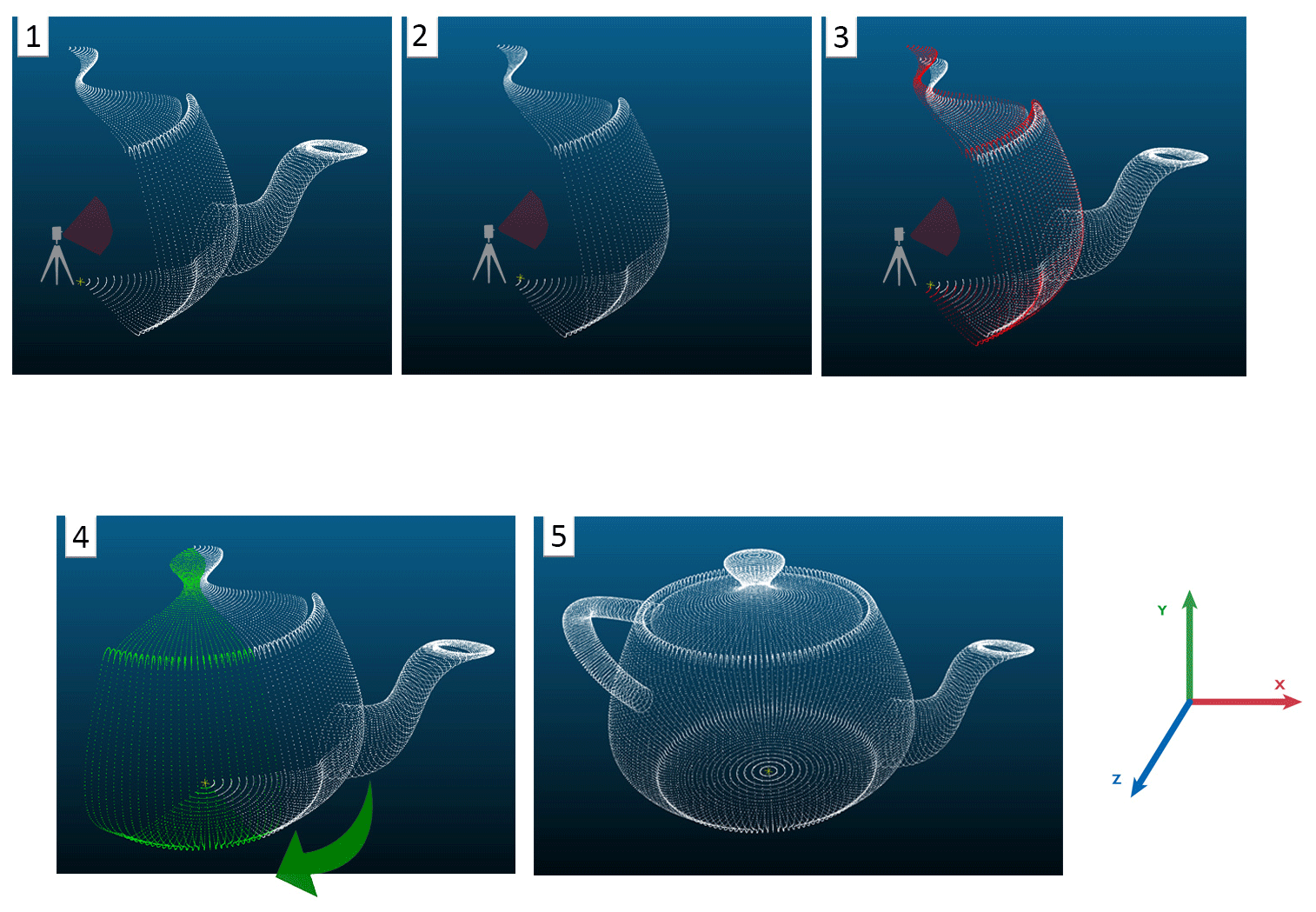
Figure 3 Steps to align the final. This is a synthetic example assuming that the lidar is located in the centre of the teapot point cloud.

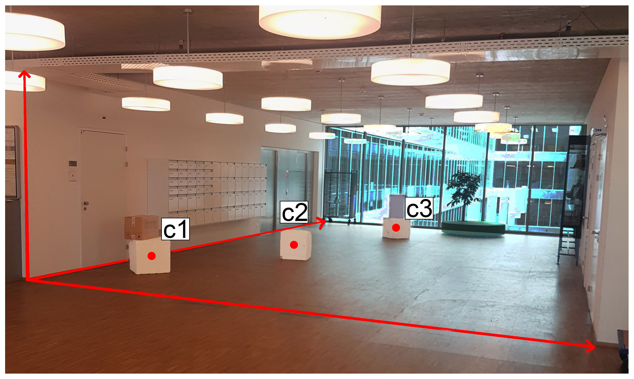
Figure 4 Picture of the scanned scene for lidar and distance comparison. The letters c1, c2 and c3 represent cubes of $\mathrm{0.5}\mathrm{m}\times \mathrm{0.5}\mathrm{m}\times \mathrm{0.5}$ m. The red arrows are the length, width and height of the ceiling.

Assuming a constant geometry of the system, we use a rigid transformation between each frame. This geometrical transformation is characterized by a 4×4 matrix:

$$T=\left[\begin{array}{cccc}a& b& c& \mathrm{0}\\ d& e& f& \mathrm{0}\\ g& h& i& \mathrm{0}\\ j& k& l& \mathrm{1}\end{array}\right],$$

with abc is the rotation applied on the x axis; def is the rotation applied on the y axis; ghi is the rotation applied on the z axis; and jkl is the translation applied on x, y and z.

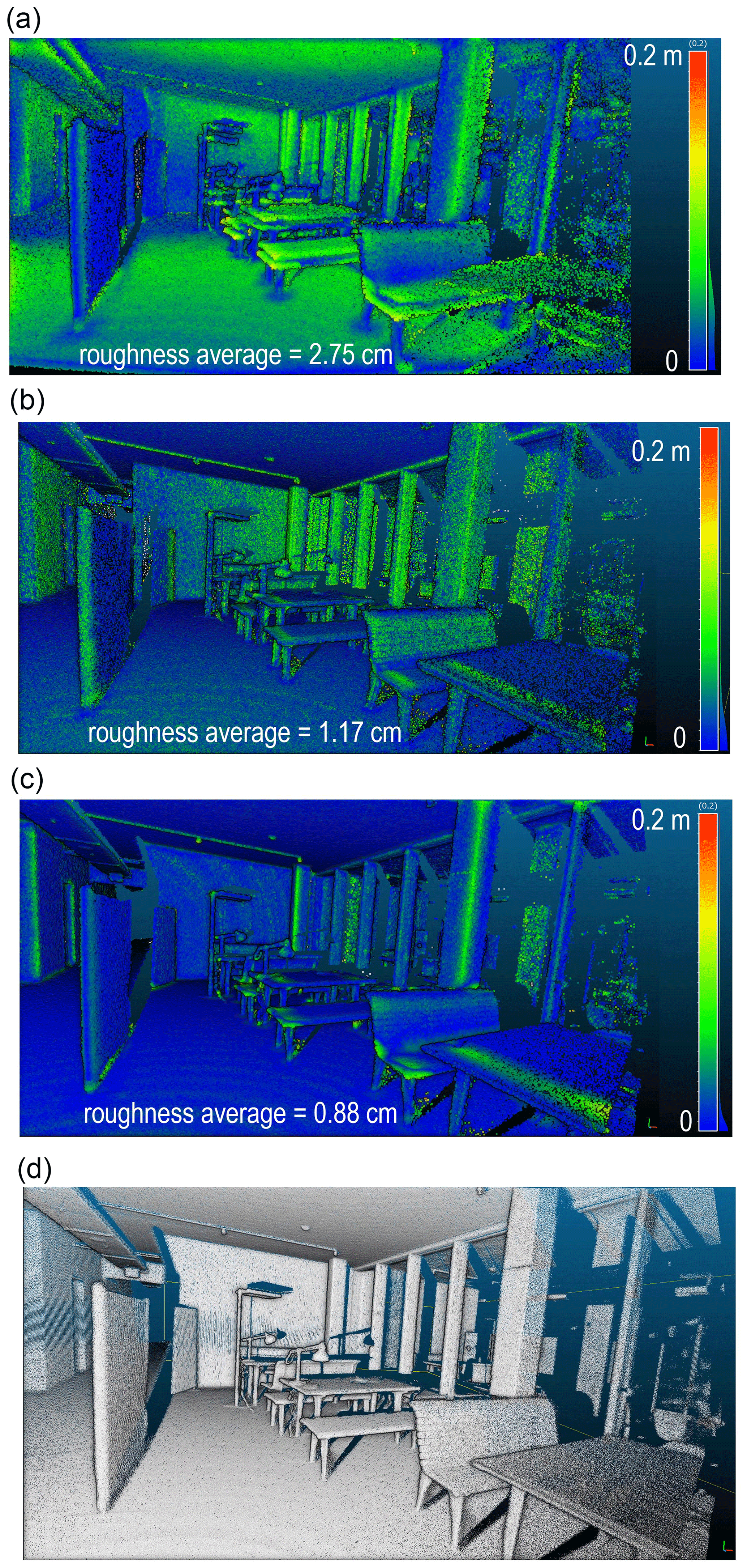
Figure 5 Point cloud roughness for adjustment steps: (a) scan without adjustments; (b) scan after adjustments of α₁ and α₂; (c) final scan; (d) final scan (EDL filter).

In our case, the rotation is applied around the y axis; the transformation matrix that aligns each frame is equal to

$$T_{\mathrm{1}}=\left[\begin{array}{cccc}\left(\cos \right(\mathit{\beta })& \mathrm{0}& \sin \left(\mathit{\beta }\right)& \mathrm{0}\\ \mathrm{0}& \mathrm{1}& \mathrm{0}& \mathrm{0}\\ -\sin \left(\mathit{\beta }\right)& \mathrm{0}& \cos \left(\mathit{\beta }\right)& \mathrm{0}\\ \mathrm{0}& \mathrm{0}& \mathrm{0}& \mathrm{1}\end{array}\right],$$

with β the angle of the motor, which depends on the time since the start of the scan and the rotation speed. Once all frames are assembled, the entire point cloud can be visualized.

As the VLP-16 Puck has the particularity of being able to scan continuously and at 360^∘, two sets of symmetrical point clouds (transit theodolite design) representing, respectively, the points with positive and negative coordinates on the x axis of the lidar reference frame (see Fig. 5a) are created, which are theoretically superposed. This observation is a crucial point of the study as it allows the adjustment of the system in order to maximize this superposition (the adjustment procedure is described in Sect. 3.2).

3.2 Post-processing and data adjustment

Since our system is custom-assembled, there is little control on exact mounting angles, which therefore require adjustments. Thus far, we have supposed that the system is turning around a fixed point corresponding to its optical centre. In fact, given that the lidar is positioned on a ball head and an L-shaped piece, it is shifted from the rotation axis. This distance was measured using an electronic caliper and is equal to 0.095 m; for each frame a translation on the z axis was applied. The affine transformation is a matrix presented as follows:

$$T_{\mathrm{2}}=\left[\begin{array}{cccc}\mathrm{1}& \mathrm{0}& \mathrm{0}& \mathrm{0}\\ \mathrm{0}& \mathrm{1}& \mathrm{0}& \mathrm{0}\\ \mathrm{0}& \mathrm{0}& \mathrm{1}& \mathrm{0}\\ \mathrm{0}& \mathrm{0}& \mathrm{0.095}& \mathrm{1}\end{array}\right].$$

Another important consideration is the correction to minimize systematic errors. Figure 2b shows two major adjustment parameters described in Neitzel (2006): α₁ for the collimation axis adjustment and α₂ for the tilting axis adjustment. The manual adjustment of these two systems involves an offset that greatly influences the point cloud geometry if uncorrected. As these offsets cannot be measured manually, an automatic adjustment is performed in post-processing. To this end, α₁ and α₂ are estimated through an optimization procedure that minimizes two functions:

1. During the rotation of the motor, the entire scene is recreated for each of the 16 scan lines. These identical scans are then put back together to form a dense point cloud. The overlap of the scans is influenced by changing the angle α₁. Thus, the first function to optimize corresponds to minimizing the average distance between the 16 full scenes that are superimposed.

2. The second function determines the angle α₂ based on the observation that both sets of symmetrical point clouds produced during the rotation must be exactly superposed. The variation in the angle α₂ creates a doming effect that tends to increase the average distance between both symmetrical point clouds (Fig. 5a). α₂ is determined by minimizing this distance.

Optimization is carried out with the Nelder–Mead method, which is based on minimizing a continuous function by evaluating points along a pattern having the shape of a simplex of dimensions equivalent to the number of parameters (Lagarias et al., 1998). The advantage of this approach is that it is derivative-free and is often appropriate when the function to minimize is discontinuous.

The resolution of the densified scan is higher near the lidar scanner and decreases away from the sensor. Because the algorithms for measuring the distance between two sets of point clouds require a lot of computational resources and must be repeated at each iteration of the Nelder–Mead optimization, the scans are downsampled using a grid average method to a uniform resolution. In addition, the optimization is carried out only for points within the distance range in the best accuracy range of 3 to 7 m (Glennie et al., 2016).

3.3 Effect of the adjustments and performance of the system

Visually, a wrong adjustment of α₁ results in blur around the scanned scene. A wrong adjustment of the α₂ angle results in a doming effect that increases away from the centre. To illustrate this, several scans were carried out in a building of the University of Lausanne. A corridor of 23 m×1.5 m was scanned and a plane was fitted on the floor surface, which is supposed to be horizontal. This plane is based on a distance interval to the lidar equivalent to the best accuracy range, i.e. between 3 and 7 m depending on the lidar performance tests (Glennie et al., 2016). This avoids the influence of points too close or too far away, which can distort the theoretical equation of the plane. In addition, the points selected for fitting the plane come from an adequate sub-sampling of the initial scan in order to standardize the density of points over the distance interval. Then, the distance of all points to this theoretical plane is evaluated, which gives an indication of the distribution of errors. Evaluation of the error as a function of the scanning distance was also measured.

Finally, reproducibility tests were performed to evaluate the stability of the system. To this end, the same scene was scanned eight times in a row. The α₁ and α₂ parameters were then estimated separately. As the system is not transported or disassembled between measurements, the aim of this test was to evaluate the stability of these parameters. The average distance between each of the eight scans is also evaluated using a multiscale model-to-model cloud comparison (M3C2 plugin in CloudCompare with its default settings) which estimates local distance between two point clouds from normal surface direction. It allows us to compute signed (and robust) distances directly between two point clouds.

3.4 Testing the system in different environments

The system has been tested in various environments. For all scans performed, the Syrp Genie Mini was configured to rotate continuously 360^∘ in 6 min. These parameters allowed the acquisition of high point resolution to maximize the information collected while maintaining a reasonable scan time. With this setting, about 10×10⁶ points per scan are collected. The first tests were carried out in a building of the University of Lausanne, which is characterized by vast surfaces and volumes. Then, the system was then used in a confined environment with no available GNSS signal: the Baulmes mines, a limestone mine abandoned at the end of the Second World War.

In these environments, several scans were assembled using the iterative closest point (ICP) alignment algorithm (Besl and McKay in 1992). This is the most popular alignment approach method for point clouds, which searches for nearest neighbours to minimize the distance between two point clouds.

3.5 Comparison with a high-cost system and field measurements

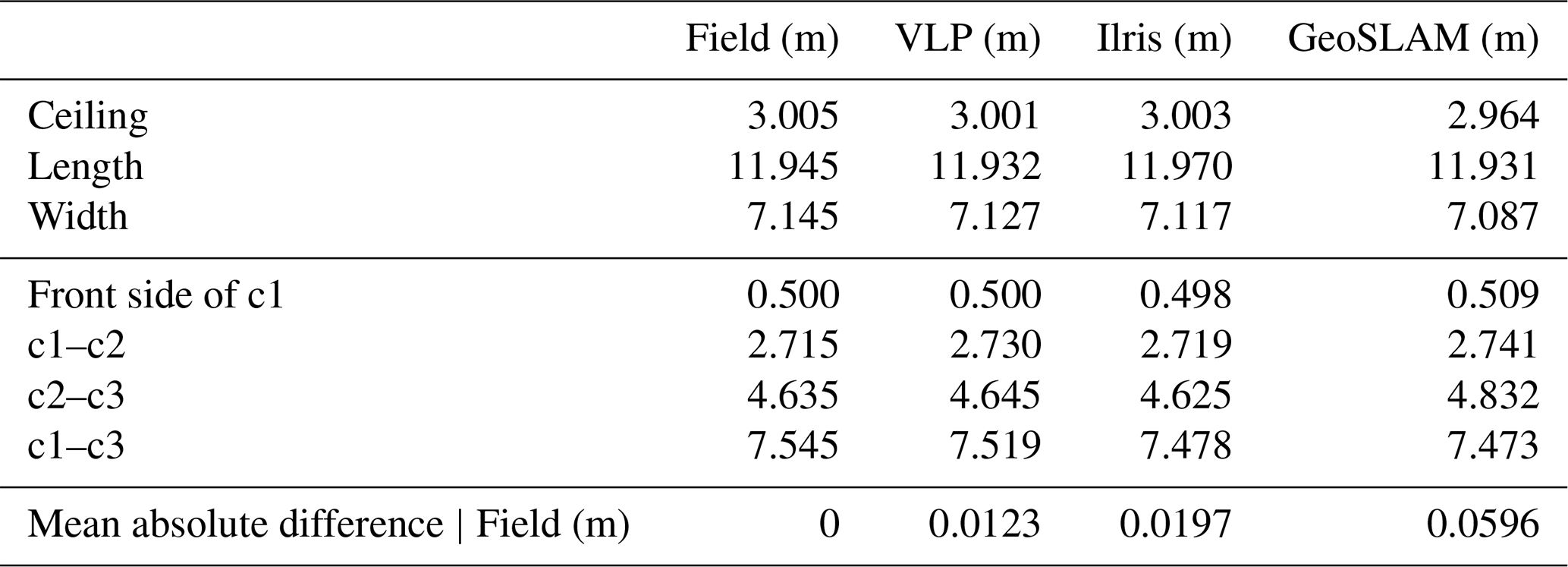
Our low-cost terrestrial lidar system was then compared to two other systems that fall into the high-cost category. These lidar systems are the Ilris 3D Optec (terrestrial laser scanner) and the GeoSLAM ZEB-REVO (mobile laser scanner with IMU tracking) (Table 3). The tests were carried out indoors and included one measurement for each system. First, Fig. 4 displays a picture of the scanned scene. As shown, objects were placed on the scene so that validation measurements could be taken with a tape measure in addition to the width and length of the corridor and the height of the ceiling. These distances were then measured for the scans coming from all three terrestrial lidar systems and compared to the measurements taken by hand. The different scans were also superimposed with an ICP algorithm to evaluate the average distance between the point clouds.

Table 3 Main characteristics of lidar used.

4 Results

All point clouds are visualized in the CloudCompare software. An EDL (Eye Dome Lighting) shading filter allowing the creation of real-time shading has been applied for better visualization (CloudCompare, 2019).

4.1 Effects of adjustments

Figure 5 shows the result of a scan that was carried out indoors in a work area of the University of Lausanne. Figure 5a shows the scene after the alignment of the different frames produced by the VLP-16 during the scan. A kind of blur caused by the splitting of the scene is observed. No processing has yet been applied, so the parameters α₁ and α₂ are set to 0. The colour scale represents the roughness of the point cloud (for a radius of 0.2 m). Figure 5b shows the scene after adjusting the α₁ and α₂ parameters. The average roughness is equal to 1.17 cm. Figure 5c shows the scene where only the scanned points corresponding to the positive coordinates on the x axis are displayed (i.e., 50 % of the data is discarded). In addition, a sub-sampling at 0.005 m is applied using a grid average method and a statistical outlier removal is performed in CloudCompare. The average roughness is equal to 0.88 cm. Figure 5d is a copy of Fig. 5c with an EDL filter.

Figure 6 shows the error corresponding to the distance of the points from the theoretical plane and the error histogram for the three adjustments steps.

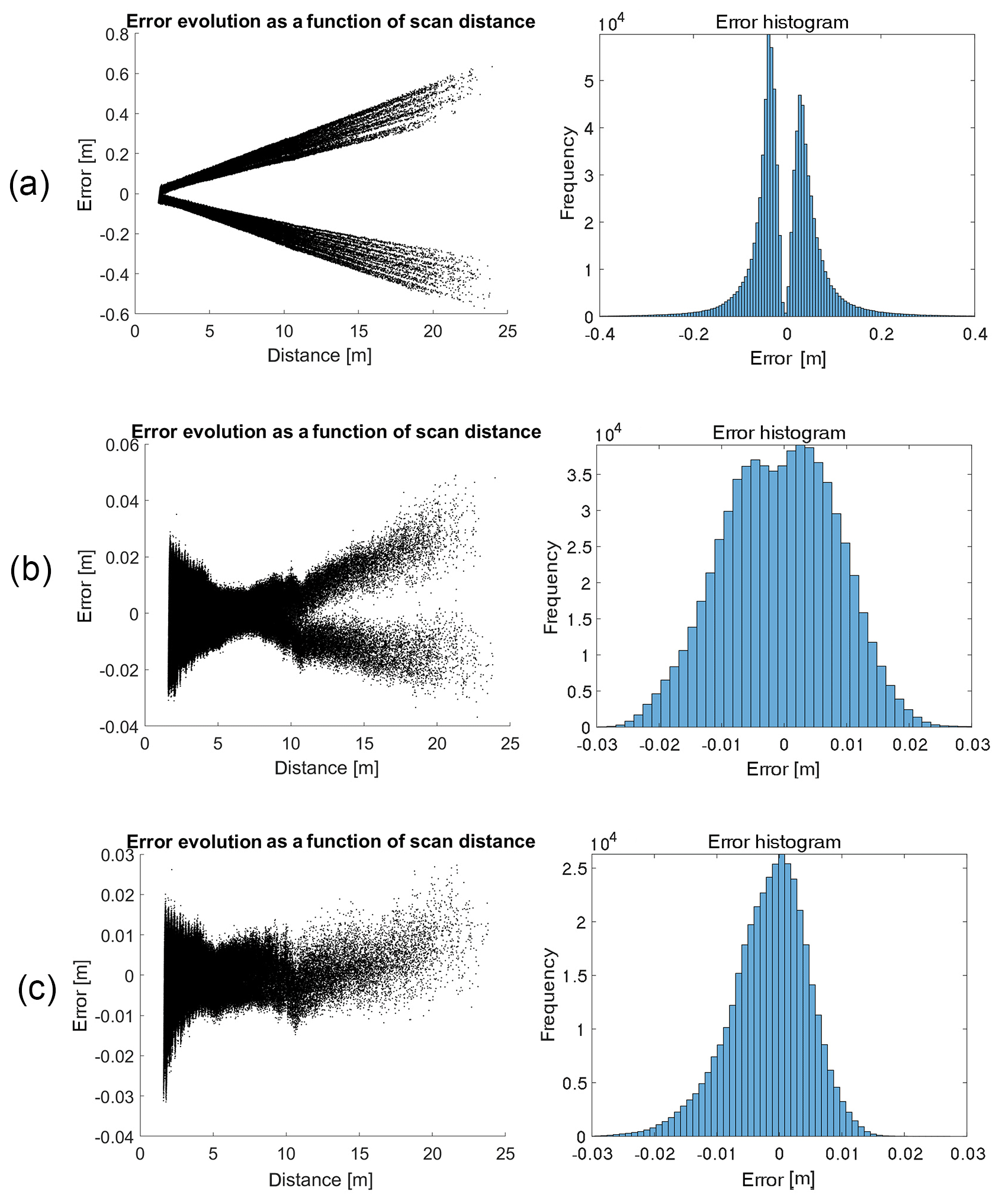
Figure 6 Effects of adjustments in relation to a theoretical plane: (a) error estimation before adjustments; (b) error estimation after adjustments; (c) error estimation after adjustments and post-treatment.

4.2 Overview of the densification quality

Figure 7a provides an overview of a scan performed indoors after adjustments. A photograph of the scanned scene with the same viewing angle is shown in Fig. 7b. Note the improvement compared to Fig. 1, where the VLP-16 was used alone.

Figure 7 Example of point cloud densification after adjustments of the system: (a) result of an indoor point cloud densification; (b) picture of the scene.

Figure 8a and b show two previews of scans performed at the Baulmes mines. Figure 8c shows the result of the registration of four point clouds in the Baulmes mines. The points corresponding to each of the acquisitions are represented in a different colour to highlight the registration. It should be noted that the clouds have not been cleaned to removed outliers, so we can see that the sensor has scanned itself. The results are characterized by a spacing set at 0.005 m and are visually realistic.

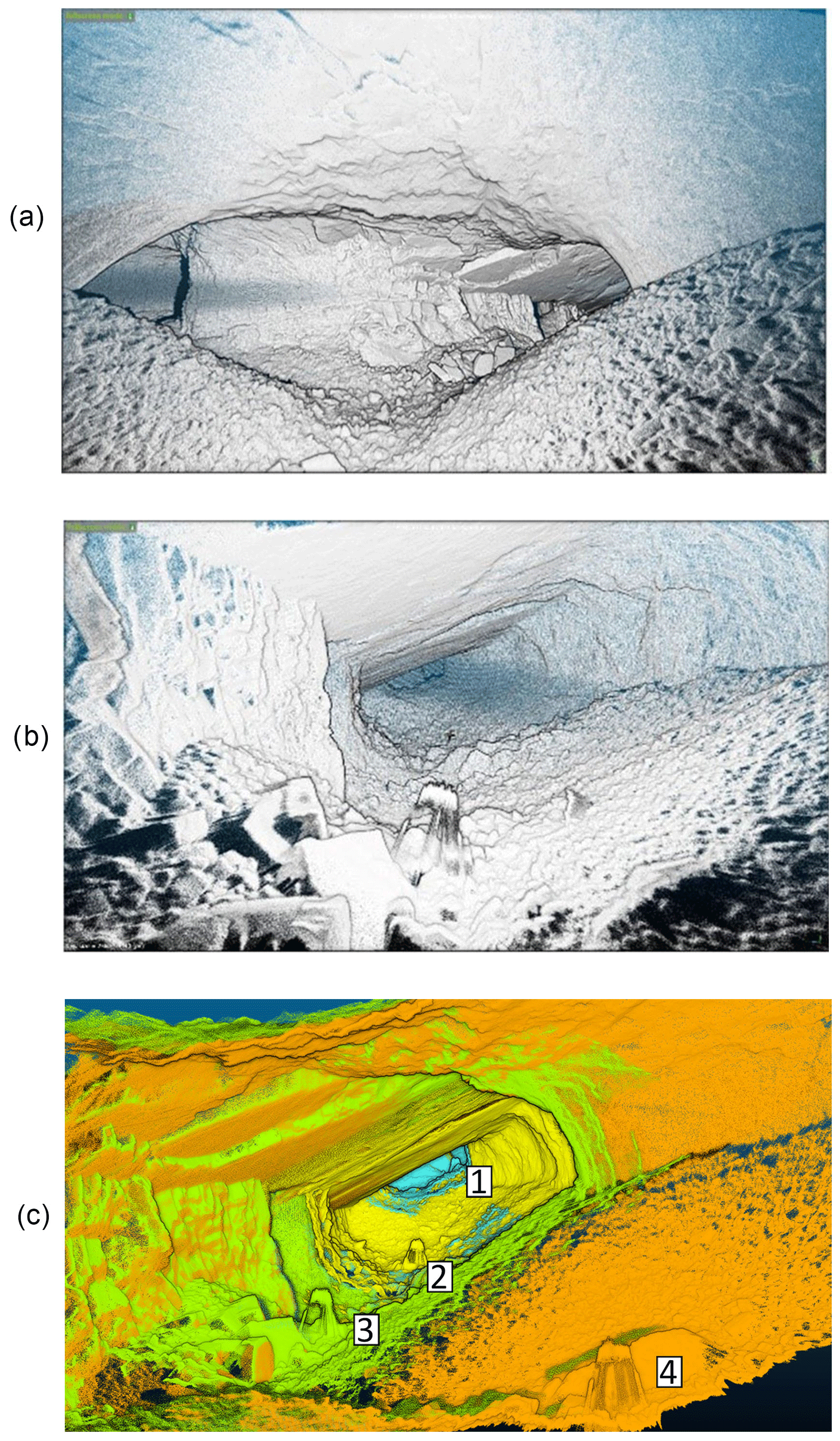
Figure 8 Scanned scenes in Baulmes mines. The height of the gallery is about 3.5 m: (a) mine example 1; (b) mine example 2; (c) point cloud registration in the mine.

4.3 Data analysis and validation

During the visualization of the point clouds, we observed the presence of an artefact in all of our measurements. Figure 9 illustrates this artefact, which is characterized by wavelets near the system that fade away with distance.

Figure 9 Artefact present near the TLS and its corresponding amplitude.

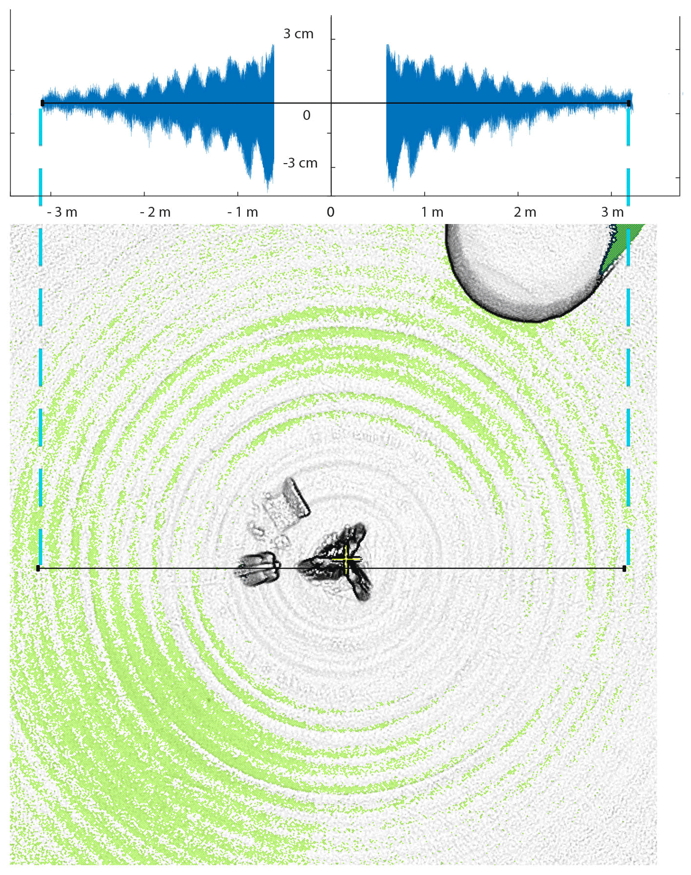
Table 4 shows the ability of the system to reproduce the same point cloud by comparing eight consecutive measurements. Each of these measurements is compared to the other seven by measuring the average distance between pairs of scans based on CloudtoCloud comparisons in CloudCompare. Table 5 shows the variation in the parameters α₁ and α₂ during this reproducibility test. Table 6 summarizes the different measurements made with the VLP-16, Ilris-3D and GeoSLAM. The data are also compared with manual measurements.

Table 4 Distance between all of the eight scans of the reproducibility test (in m).

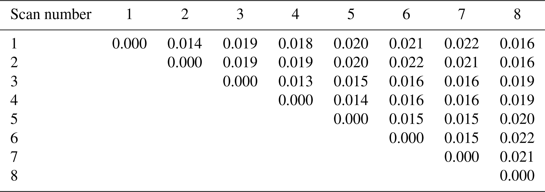
Table 5 Variability of α₁ and α₂ parameters during reproducibility test.

Table 6 Comparison of field and lidar measurements (see Fig. 4). Vertical line stands for “in comparison with”.

To validate the registration, the comparison of the distances between the points coming from our assembly and those coming from GeoSLAM was carried out using CloudCompare with the option “Cloud to cloud distance”. The average distance between both point clouds and the SDs of these distances are shown in Table 7.

Table 7 Mean distance between Ilris, GeoSLAM and Velodyne TLS (M3C2 distance).

5 Discussion

5.1 Data analysis before and after the adjustment of parameters α₁ and α₂

As shown in Fig. 5, adjustment is a fundamental step in producing accurate 3-D modelling of an environment.

The use of the two symmetrical datasets produced during an acquisition using the VLP-16 is a key element in the optimization of the system. However, as shown in Fig. 5b, the roughness calculation tells us that the entire point cloud could still be smoother. For this reason, we decided to keep only half of the points (Fig. 5c and d) in order to obtain a sharper representation of the scene. This choice will be justified after the following analysis.

The error depends on the distance to the lidar. Before adjustment, the distance to the theoretical plane varies from about ±4 cm (μ±1σ) for the closest points to the lidar to 59 cm (μ±1σ) for a scan distance of 23 m (Fig. 6a). After adjustment of parameters α₁ and α₂, the entire point cloud approaches the theoretical surface, as shown in Fig. 6b. However the evolution of the error as a function of distance is still not constant and tends to increase linearly with the scan distance. The minimum error is logically in the point range where the theoretical plane is situated. The bimodal error histogram shown in Fig. 6b and centred at ±0.5 cm shows that the superposition between the two halves of the scan is still not entirely accurate despite the adjustment performed.

The evolution of the error as a function of the scanning distance when keeping only one half of the scan (Fig. 6c) shows an accuracy range of ±2.5 cm (μ±1.5σ), which remains within the accuracy range given by Velodyne. The post-processing steps and the adjustment of mounting angles has allowed us to drastically reduce errors; however, the adjustment parameters vary greatly between scans, as shown in Tables 5 and 6. This can be explained by the assembly of our lidar system being relatively unstable. The impact of the adjustment, and particularly the need to repeat the self-adjustment of α₁ and α₂, could be alleviated by welding together the different components of the system.

5.2 Performance and stability of the TLS

According to the manufacturer's website, the VLP-16 Puck allows data acquisition at a distance of 100 m for an accuracy of ±3 cm, under optimal acquisition conditions. Various stability tests have been carried out in a metrology laboratory, which indicate an accuracy of ±2 cm for an acquisition distance of 5 m to a white and flat target (Glennie et al., 2016).

Reproducibility tests tell us that the system is quite stable when it is not moved or disassembled. The α₁ adjustment parameter shows a slight variation for scans 1, 2 and 8. This can be explained by the Nelder–Mead algorithm, which finds a local and not a global minimum of the function. The use of this algorithm is nevertheless privileged because of its efficiency in terms of computing time.

The calculation of the average distance between all scans (Table 4) indicates a small variation in the scanned scene. The measured distances are mostly below 2 cm, confirming the tests performed by Glennie et al. (2016) and may be related to noise. We can see a correlation between scan pairs having similar adjustment parameters (scans 1, 2, 8) and their average distances.

5.3 Comparison with high-cost hardware and field measurements

The measurements taken manually in the field have enabled comparisons with the scans obtained with our system. Table 6 shows that the measurements taken with the VLP-16 TLS are closest to ground truth, with an average of 1.23 cm compared to 1.97 cm for the Optec system and 5.96 cm for GeoSLAM. This result should be treated with caution as it may be specific to our experimental setup. It should also be taken into account that a sub-sampling at 0.5 cm from the scans was performed using a grid average method.

After alignment using an ICP algorithm, the scans could be compared and are presented in Table 7. Assuming that the Optec system is the most accurate, our system achieves a good performance with an average distance of ±2.5 cm. GeoSLAM obtains a lower level of accuracy with an average of ±6.7 cm.

5.4 Origin of the short-range artefacts

Visually, this artefact is easily observed in the results of scans near the tripod, when data were acquired on a flat surface. Figure 9 shows the influence of this artefact on the scan. We notice that the error spreads in the form of regular waves and fades away as it moves away from the lidar. It has a magnitude of 3 cm closest to the lidar and drops below 1.5 cm at a distance of 3 m. The wave frequency is about 20 cm. A hypothesis on the origin of this artefact would be related to the length of the arm, which was measured manually. It turns out that errors in the length of the arm have no influence on the occurrence of these artefacts but instead create horizontal deformations. We also tested this by using each laser separately, by using another tripod, and by varying the parameters and changing the motor speed. However, the artefacts remain constant (same distance and amplitude between waves). This indicates that the artefacts seem to be related to the lidar itself. Since the error appears to be regular, it would be conceivable to correct outliers by modifying each point according to the distance from the lidar.

6 Conclusions

This paper presents a low-cost terrestrial lidar system based on the use of a Velodyne VLP-16. Comparisons with high-precision models allow validating the accuracy of the system, which seems promising. As shown in the results, our system requires adjustment for each scan performed. These adjustments are made in post-processing and are possible thanks to the data acquisition geometry of the VLP-16. This could be avoided if the system components were welded together. However, we wanted to keep the possibility of separating these elements in order to use the lidar for other projects, for example. The use of the lidar system in an underground mine demonstrates the potential applications of such a system, in particular in the field of geosciences.