the Creative Commons Attribution 4.0 License.
the Creative Commons Attribution 4.0 License.
 | 27 Jan 2021
Error estimate for fluxgate magnetometer in-flight calibration on a spinning spacecraft
Yasuhito Narita
Ferdinand Plaschke
Werner Magnes
David Fischer
Daniel Schmid
Fluxgate magnetometers are widely used for in situ magnetic field measurements in the context of geophysical and solar system studies. Like in most experimental studies, magnetic field measurements using the fluxgate magnetometers are constrained by the associated uncertainties. To evaluate the performance of magnetometers, the measurement uncertainties of calibrated magnetic field data are quantitatively studied for a spinning spacecraft. The uncertainties are derived analytically by perturbing the calibration parameters and are simplified into the first-order expression including the offset errors and the coupling of calibration parameter errors with the ambient magnetic field. The error study shows how the uncertainty sources combine through the calibration process. The final error depends on (1) the magnitude of the magnetic field with respect to the offset error and (2) the angle of the magnetic field to the spacecraft spin axis. The offset uncertainties are the major factor in a low-field environment, while the angle uncertainties (rotation angle in the spin plane, sensor non-orthogonality, and sensor misalignment to the spacecraft reference directions) become more important in a high-field environment in a proportional way to the magnetic field. The error formulas serve as a useful tool in designing high-precision magnetometers in future spacecraft missions as well as in data analysis methods in geophysical and solar system science.
- Article
(1381 KB) - Full-text XML
- BibTeX
- EndNote


Fluxgate magnetometers perform measurements from DC (direct current) to low-frequency magnetic field vectors (typically up to 10–100 Hz) and are widely applied to in situ spacecraft observations for space plasma, magnetospheric, and heliospheric research (Acuña, 2002). The fluxgate magnetometers can be mounted on a spinning spacecraft or a three-axis stabilized one, depending on the individual mission concept. In particular, in-flight calibration benefits from the spacecraft spin, since 8 of 12 calibration parameters are determined by making use of the spacecraft spin. Detailed procedures for the in-flight calibration on a spinning spacecraft are presented by, e.g., Kepko et al. (1996) and Plaschke et al. (2019).
The goal of the current paper is to give an outline of systematic errors of calibrated fluxgate magnetometer data on a spinning spacecraft. The error of magnetic field data occurs due to the uncertainties of the calibration parameters. The error sources may combine with one another through the calibration process. We derive the full expression of calibration errors as well as a more practical, simplified expression by truncating at the first order of relative errors. The scope of our work is the error estimate of calibrated magnetometer data in a low-field environment. In practice, more effects need to be taken into account, including sensor nonlinearities, temperature dependence (temperature drift effect), and jumps in the data associated with the change in operational modes.
For a spin-stabilized spacecraft, the magnetometer in-flight calibration is performed by correcting for offsets (including the spacecraft DC field), gains, deviations from the ideal orthogonal coordinate system, spacecraft spin-axis direction with respect to the sensor reference direction, and rotation angle around the spacecraft spin axis. For a nearly orthogonal unit-gain sensor system, the measured magnetic field is transformed into a de-spun coordinate system and is expanded into a Fourier series over the frequencies as
for the ith component of the magnetic field. Fi is the Fourier coefficient, i the imaginary unit, ω the de-spinning frequency (as angular frequency), N the number of data points, and t the time in the data.
The magnetic field vector measured by the three sensors (sensor output) is related to the ambient field by taking account of spacecraft spin-axis direction, spacecraft spin phase, sensor-axis directions, sensitivities (or gains) of the sensors, and offsets (Kepko et al., 1996; Plaschke et al., 2019). The relation is constructed in the following fashion.
-
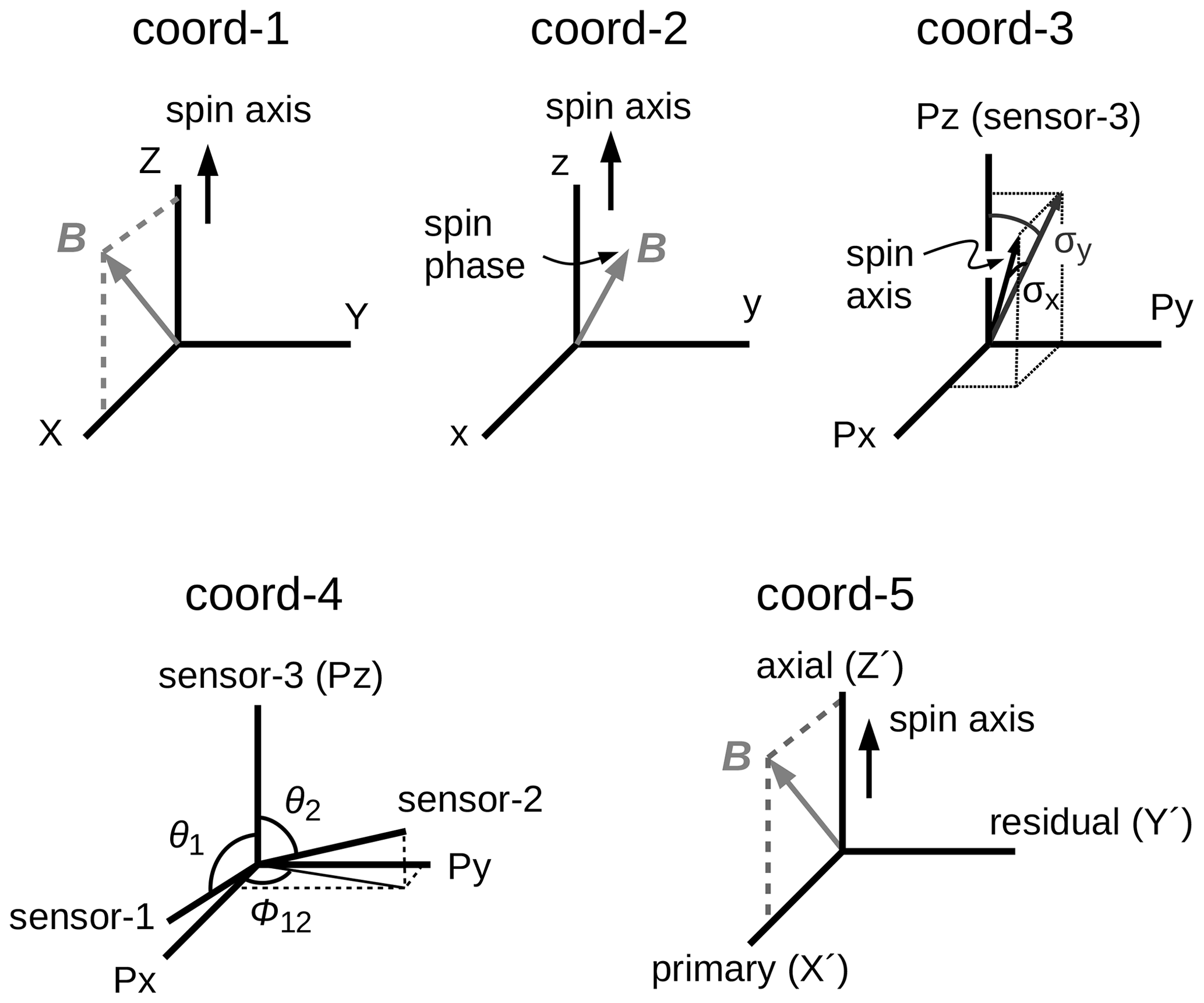
The true or model ambient field is set in the inertial (i.e., non-spinning) orthogonal spacecraft spin-axis-aligned coordinate system (the coord-1 system in Fig. 1) with the spin-plane component in the X direction (BX=Bp) and the spin-axis component in the Z direction (BZ=Ba). There is no magnetic field in the rest spin-plane component, BY=0, because the coord-1 system spans the spacecraft spin axis (in the Z direction) and the ambient field in the X–Z plane. The magnetic field is modeled in the coord-1 system as
-
The model ambient field in the coord-1 system is transformed into the spinning orthogonal spin-axis-aligned system (the coord-2 system in Fig. 1) with the magnetic field components Bx, By, and Bz by referring to the spin axis as the z direction and rotating the spin plane around the spin axis by the spacecraft spin phase −ωt (here ω is defined as the de-spinning frequency and −ω as the spin frequency; t the time) as
The magnetic field vector in the coord-2 system is symbolically related to that in the coord-1 system as
where Ω−1 is the spin rotation matrix. Note that Ω is defined as the de-spinning matrix here.
-
The field is then transformed into the spinning, orthogonal sensor package system (the coord-3 system in Fig. 1) first by rotating around the spin axis by correcting for the magnetometer boom extension and a possible misalignment of the fluxgate sensor in the spin plane (with the rotation angle ϕa in the xy plane around the spin axis in the coord-2 system) and then by orienting the Pz axis in the sensor-3 direction with the spin-axis tilt angles σPx and σPy (with respect to the Pz axis) to obtain the magnetic field components as BPx, BPy, and BPz (here, P in the subscript stands for the sensor package). Here, σPy is the angle between the Pz axis and the projection of the spin axis on the (Pz,Py) plane. σPx is the angle between the spin axis and the (Pz,Py) plane. The magnetic field vector in the coord-3 system is symbolically related to that in the coord-2 system as
where Φ−1 is the azimuthal rotation matrix in the spin plane (around the spin axis in the coord-2 system) and Σ−1 is the transformation matrix to orient the z axis in the direction to the sensor package Pz direction. Again the matrices without inversion are used for the reconstruction of the model magnetic field in the calibration.
-
The field is further transformed into the spinning, non-orthogonal sensor-axis-aligned system (the coord-4 system in Fig. 1) by correcting for the elevation angles θ1 (between the sensor-1 and the sensor-3 directions) and θ2 (between the sensor-2 and the sensor-3 directions) and also for the azimuthal separation angle ϕ12 (between the sensor-1 and sensor-2 projected onto the plane normal to the sensor-3 direction) to obtain the magnetic field components B1, B2, and B3 in the directions of the sensor axes including the gains and the offsets. The magnetic field vector in the coord-4 system is symbolically related to that in the coord-3 system as
where Γ−1 is the transformation matrix using three angles (θ1, θ2, and ϕ12), G−1 is the gain matrix, and Os is the offset vector.
-
Finally, in the calibration procedure, the above transformations are inverted to estimate the ambient field from the sensor output. The estimated or reconstructed field is expressed in the de-spun inertial coordinate system (the coord-5 system in Fig. 1) with the spin-plane primary component (), spin-plane residual component (), and spin-axis component (). The primed field expression in the coord-5 system (, , and ) is identical to the model ambient field BX, BY, and BZ in the coord-1 system if the calibration parameters are all accurately known. The model magnetic field is reconstructed from the sensor magnetic field as
If the calibration parameters are all known, the reconstructed field Bc5 restores the model field Bc1.
Note that the forward transformation is defined for the conversion of the sensor output (in the coord-4 system) into the magnetic field in the physically relevant system (the coord-1 system). In the error estimate study, the inverse transformation from the coord-1 system to the coord-4 system is more instructive in order to compare the calibrated magnetic field vector in the coord-5 system with the model ambient field in the coord-1 system.
The relation between the sensor-output magnetic field Bs=Bc4 (introduced in the coord-4 system) and the model ambient field in the spinning frame Bc2 (introduced in the coord-2 system, Eqs. 3–5) is expressed by a set of transformation matrices and an offset vector Os as in Plaschke et al. (2019):
Here, the set of transformation matrices is composed of (1) the inverse rotation matrix around the spin axis Φ−1 by the rotation angle ϕa, (2) the inverse rotation matrix Σ−1 correcting for the tilt of spacecraft spin axis to the Pz direction (transforming the coord-2 system into the coord-3 system), (3) the inverse conversion matrix Γ−1 (transforming the coord-3 system into the coord-4 system), and (4) the inverse gain matrix G−1. The sensor-output field is then corrected for the offset vector Os in the sensor-axis directions. The matrices are constructed as follows (Plaschke et al., 2019).
The calibrated magnetic field vectors depend on the ambient magnetic field (Bp in the spin plane and Ba along the spin axis) and the following calibration parameters:
-
gain ratio g between the two spin-plane sensors
-
absolute gains in the spin plane Gp and that in the spin-axis direction Ga
-
offsets in the three sensor directions O1, O2, and O3
-
spin-axis tilt angles σPx and σPy in sensor package system (σPy is the angle between the sensor-3 direction and the projection of the spin axis onto the sensor package Py–Pz plane; σPx is the angle of spin axis and the sensor package Py–Pz plane)
-
deviation of elevation angles from 90∘ defined as δθ1 and δθ2, for the sensors 1 and 2, respectively
-
deviation of azimuthal angle from 90∘ defined as δϕ12
-
rotation angle ϕa in the spin plane.
Note that the orthogonality nearly holds such that the elevation and azimuthal angles exhibit only a small deviation from 90∘:
Also the tilt angles are small and close to zero:
The relative gain and the two absolute gains are close to unity:
The sensor output in the de-spun coordinate system (including the temperature dependence) is expressed up to the second-lowest order of the spin frequency as in Plaschke et al. (Eqs. 24–26 in 2019):
Here, the magnetic field vector (, , ) is represented in the coord-5 system and hence ideally reproduces the model magnetic field in the coord-1 system. That is, the z component is in the direction of spacecraft spin axis and the x component is is in the spin plane. The y component is also in the spin plane but should ideally not contain the ambient field. If the calibration parameters were all accurately known, the residual component () would be zero and the ambient field reproduced or reconstructed by the calibration would have the spin-plane component () and the spin-axis component (). The directions of the three components are orthogonal if the calibration is accurate. Non-orthogonality may arise due to the uncertainties in the calibration parameters. The spacecraft spin frequency ω (as angular frequency) is assumed to be well known. t denotes time in Eqs. (23)–(25). We also assume that the calibration parameters do not change over time or along the spacecraft orbit.
2.1 Spin-plane primary component
The systematic error of magnetic field data is analytically derived by perturbing the calibration equations (Eqs. 23–25). The error in the X′ component (spin-plane primary component) is denoted by . The spin-plane primary component is assumed to be aligned with the ambient field direction in the spin plane after calibration. On the assumption of the constant spin frequency , the error is derived by perturbing Eq. (23) as follows:
Here, the function max(x,y) returns the larger value from two variables, x and y, and is defined as
The function max(x,y) takes the largest amplitude from an elliptically shaped time series signal such as xcos (ωt)+ysin (ωt). After differential calculus (see Appendix), the expression of error is arranged to that of calibration parameters (gains, offsets, and angles):
It is useful to introduce the following variables to simplify the notations:
If the gains (both absolute and relative ones) are close to unity (g≃1, Gp≃1) and the misalignments are small (σPx≪1 rad, σPy≪1 rad, δθ1≪1 rad, δθ2≪1 rad, δϕ12≪1 rad), Eq. (28) is simplified with the leading terms:
We assume (which is realized when ϕa≤1 holds), then Eq. (32) is further simplified into a more practical form:
2.2 Spin-plane residual component
Derivation of the error in the Y′ component (which is residual to the primary component after determination or reconstruction of the ambient field in the spin plane) nearly follows that in the X′ component. Note that the Y′ component only has a tiny amount of the ambient field because of its residual character. The Y′ component vanishes if the calibration is properly and accurately done. After derivative calculations (see Appendix), the error of the residual component is estimated as
Equation (34) is sorted to the errors of calibration parameters as
Again, as done in the calculation of the X′ component, we take the leading terms (the first-order terms) and obtain a simplified expression of the error of the residual component as
The differences from (Eq. 33) are 2Δ(δϕ12) and Δϕa in the second term in Eq. (36). The appearance of Δϕa means that the uncertainty of the magnetometer boom extension angle (the spin-plane rotation angle) causes a finite residual component; that is, the spin-plane ambient field is erroneously projected to yield the residual component Y′ by an angle of Δϕa. The effect of Δϕa on the spin-plane primary field component is of the second order, while that on the residual component is of the first order. According to our estimate of the calibration parameter errors (Table 1), the first-order errors are in the range between 10−2 and 10−4 and the second-order errors (due to the couplings of calibration errors with the other small parameters) are in the range between 10−5 and 10−8.
2.3 Spin-axis component
The error of spin-axis component is derived from Eq. (25) in a straightforward fashion:
For a nearly unit gain in the axial direction (Ga≃1) and small misalignments (σPx≪1, σPy≪1), the expression of error estimate is simplified into
Equation (39) indicates that an error occurs in the spin-axis direction (1) when the offset ΔO3 is present, (2) when the axial (absolute) gain Ga has an uncertainty, or (3) when the spin-axis angle relative to the sensor Z direction has an uncertainty (which introduces a mixing or projection of the spin-plane component by the spin-axis component).
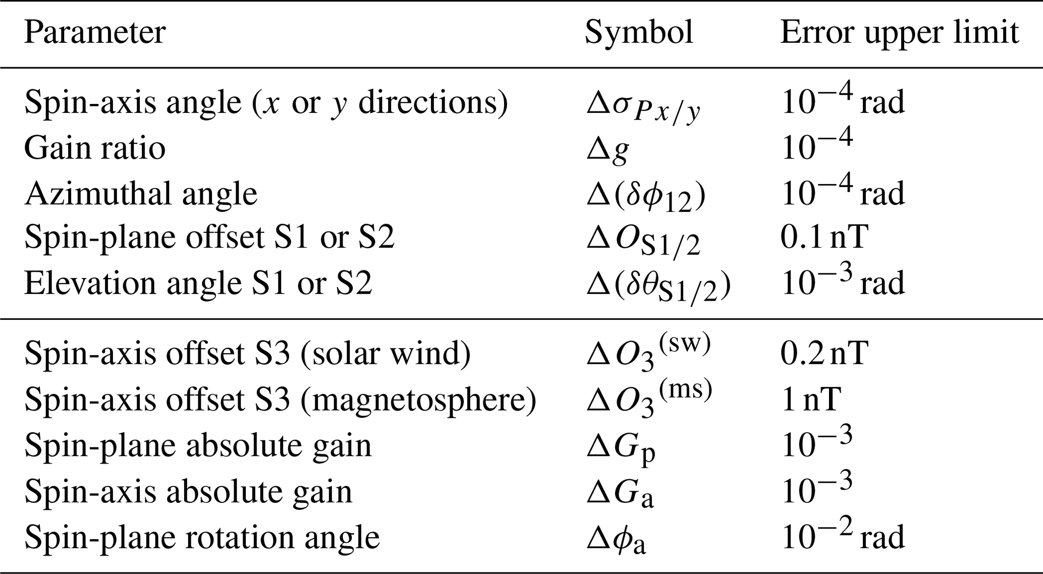
Nominal errors (as upper limits) of calibration parameters are summarized in Table 1 as lessons from Earth-orbiting spinning spacecraft Cluster (Escoubet et al., 2001; Baloghet al., 2001), THEMIS (Time History of Events and Macroscale Interactions during Substorms) (Angelopoulos, 2008; Auster et al., 2008), and MMS (Magnetospheric Multiscale) (Burch et al., 2016; Russell et al., 2016).
The spin-plane-related calibration parameters are assessed in detail by Plaschke et al. (2019). The accuracy studies on the spin-axis offset are presented by Alconcel et al. (2014), Frühauff et al. (2017), Plaschke (2019), and Schmid et al. (2020). In the following, we review the uncertainties of calibration parameters.
Table 1Nominal errors of calibration parameters. The five lines at the top (spin-axis angles, gain ratio, azimuthal angle, spin-plane offsets, and elevation angles) represent the in-flight calibration for THEMIS (Plaschke et al., 2019). The nominal error of spin-axis offset may vary between 0.2 nT in the solar wind (Plaschke, 2019) and 1 nT in the magnetosphere from temperature drift studies by Alconcel et al. (2014) and Frühauff et al. (2017). Absolute gains in the spin plane and along the spin axis are taken from the ground calibration experience. Spin-plane rotation angle is taken from the magnetometer boom design for BepiColombo Mio.
3.1 Offset error
The offsets in the spin plane (O1 and O2) are determined by the in-flight calibration. The error of spin-plane offsets on in-flight calibration is, after Plaschke et al. (2019), minimized down to the sum of (1) spin-plane component of natural fluctuation at the spin frequency (denoted by Fp), (2) the projection of the spin-axis ambient field by an error of spin-axis angle BaΔσPx∕y, and (3) the projection of the spin-axis ambient field by an error sensor elevation angle BaΔ(δθS1∕2):
The lesson from the in-flight calibration for the THEMIS magnetometer data indicates that an offset value of about 0.1 nT or better (i.e., smaller) can be reached using spacecraft spin (Plaschke et al., 2019).
The offset in the spin-axis direction cannot be determined from the spacecraft spin but needs to be determined in different ways, for example, using additional measurements such as absolute magnetic field magnitude (Nakamura et al., 2014; Plaschke et al., 2014) or using plasma physical properties such as the nearly incompressible fluctuation nature in the solar wind (Hedgecock, 1975; Leinweber et al., 2008), the highly compressible fluctuation nature in which the fluctuations are nearly aligned with the ambient field (Plaschke and Narita, 2016; Plaschke et al., 2017), or the magnetic null environment in diamagnetic cavities around comets (Goetz et al., 2016a, b). The uncertainty in the spin-axis offset can empirically be minimized to 0.2 nT when using the solar wind fluctuations (Plaschke, 2019) and the mirror-mode fluctuations (Plaschke and Narita, 2016; Frühauff et al., 2017). The accuracy of spin-axis offset determination can be improved when a larger amount of data is available. An accuracy of 0.5 nT or 1.0 nT is regarded as representative using the mirror-mode fluctuations (Schmid et al., 2020). It is also worth noting that the offset drift is up to 1 nT per year as lessons from Cluster (Alconcel et al., 2014) and THEMIS (Frühauff et al., 2017), which may be used as a nominal value of spin-axis offset error when the spacecraft stays in the magnetosphere and the in situ offset determination using solar wind or mirror-mode fluctuations is not possible.
3.2 Gain error
The error of gain ratio in the spin plane is minimized to the natural fluctuation amplitude at the second harmonic of spin frequency in the spin plane (denoted by F2p) relative to the spin-plane ambient field Bp (Plaschke et al., 2019):
The gain ratio can be determined to a reasonably accurate level using the spacecraft spin, down to an uncertainty of about 10−4 (Plaschke et al., 2019). It is true that the gain ratio in the spin plane g is related to the sensitivity measurements during the ground calibration through
where Sx and Sy are the sensitivity (absolute gain) of the two spin-plane sensors, but the gain ratio obtained from the in-flight calibration is sufficiently accurate () in practical applications.
3.3 Sensor-axis non-orthogonality
Sensor-axis non-orthogonality includes errors of the elevation angles Δ(δθ1) and Δ(δθ2) and azimuthal angles between S1 and S2 Δ(δϕ12). The error of elevation angles Δ(δθ1) and Δ(δθ2) is, after Plaschke et al. (2019), minimized to the sum of (1) natural frequency at the spin frequency relative to the ambient spin-axial field, (2) offset error relative to the ambient spin-axial field, and (3) uncertainty of the spin-axis angle as
The elevation angles Δ(δθ1) and Δ(δθ2) are the angles between the sensors S1 and S3 and between S2 and S3, respectively. The angle uncertaintiesΔ(δθ1) and Δ(δθ2) can be obtained both from the ground calibration and from the in-flight calibration. Errors of the elevation angles are about 10−3 in the in-flight calibration (Plaschke et al., 2019).
The azimuthal angle deviation δϕ12 is also related to the ground-calibrated sensor angles ξ12, ξ13, and ξ23. By using the trigonometric relations, it is straightforward to show that the relation is
For smaller deviation angles of ϕS12, ξ12, ξ13, and ξ23 (i.e., if the sensors are nearly orthogonal to one another), the relation is simplified into
The azimuthal angle δϕS12 can thus be obtained both from the ground calibration and from the in-flight calibration, and its uncertainty can be sufficiently minimized down to about 10−4 rad in the in-flight calibration (Plaschke et al., 2019).
3.4 Misalignment to the spacecraft reference direction
Angular deviation of the spin axis from the normal direction of the sensor x–y plane is characterized by two angles: σPx and σPy. The error of misalignment angles σPx and σPy is estimated as the ratio of the spin-axis natural fluctuation amplitude at the spin frequency to the spin-plane ambient field,
and the value of σPx∕y is empirically about 10−4 rad (Plaschke et al., 2019). The angles σPx and σPy need the determination or knowledge of spacecraft spin axis and cannot usually be evaluated during the ground calibration of the sensors.
The remaining angle is the rotation angle in the spin plane The rotation angle can be determined in flight using Earth's magnetic field model in the case of Earth-orbiting spacecraft, and the method works better in a high-field environment. For example, the rotation angle is determined to an accuracy of 0.5∘ or better when using the magnetic field data around the perigee with a field magnitude of about 8000 nT. In-flight determination of the rotation angle is meaningful when the accuracy in the in-flight method is better than the knowledge from the boom design with ground verification. We take the case of the BepiColombo Mio magnetometer because the magnetometer boom extension direction is known to be within an uncertainty of 0.5∘ (which gives ) from the spacecraft design and ground verification. As we will see in the next section, the uncertainty of rotation angle in the spin plane plays an important role in the final error estimate in a high-field environment.
The individual error sources are combined using the first-order expressions (Eqs. 33, 36, and 39) to evaluate the error of calibrated magnetometer data for the nominal parameters (Table 1). Here, the errors represent the upper limits of the three magnetic field data in three directions (spin-plane primary, spin-plane residual, and spin-axis components). For a practical purpose, the combined errors in Eqs. (33), (36), and (39) are reformulated in an approximate form using the values given in Table 1:
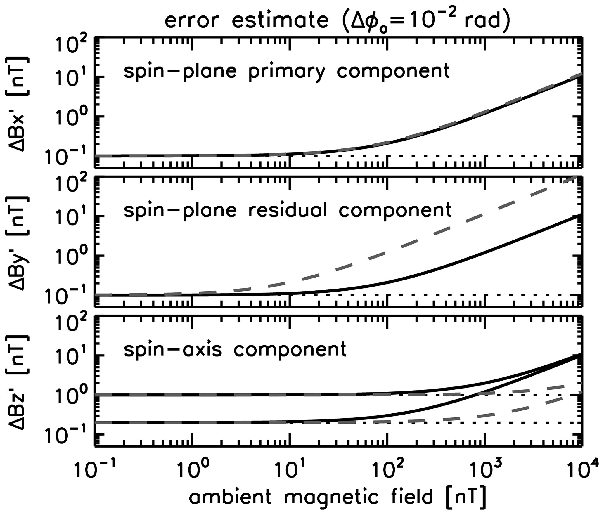
The combined errors are graphically displayed in Fig. 2 as a function of the ambient magnetic field in the spin-axis direction (0∘, data curves in black) and spin-plane direction (90∘, data curves in gray).
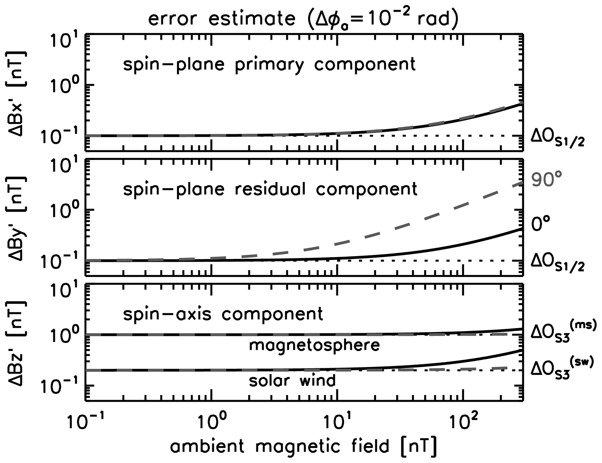
Figure 2Error of in-flight calibrated magnetometer data for an error of magnetometer boom angle (the case for the BepiColombo Mio magnetometer). Curves in black and in gray represent for the axial ambient magnetic field (0∘ to the spin axis) and the spin-plane ambient field (90∘), respectively.
Equations (33), (36), and (39) and Fig. 2 indicate that the calibration error has two distinct domains: (1) the offset-dominant domain in a low-field, up to an ambient field of about 1 nT when the field is along the spin axis (curves in black in Fig. 2), and up to 10 nT when the field is in the spin plane (curves in gray in Fig. 2) and (2) the ambient field-dependent domain in a high field (above 1 or 10 nT). In the low-field case, the offset dominates the magnetometer data error and the offset value is expected to be in the range between 0.1 to 1 nT. In the high-field case, the error grows linearly with the ambient field and the relative error is expected to be between 1 % (which comes from Δϕa) and 0.1 % (which comes from the absolute gain error and the elevation angle error).
The error depends on the angle between the ambient field and the spacecraft spin axis. The gain errors, azimuthal angle error, and boom misalignment are coupled to the spin-plane ambient field in the spin-plane components (Eqs. 33 and 36). The spin-axis misalignment and elevation angle errors are coupled to the spin-axis field. The axial gain and the spin-axis misalignment are coupled to the spin-axis and spin-plane ambient field, respectively, in the expression of spin-axis component (Eq. 39).
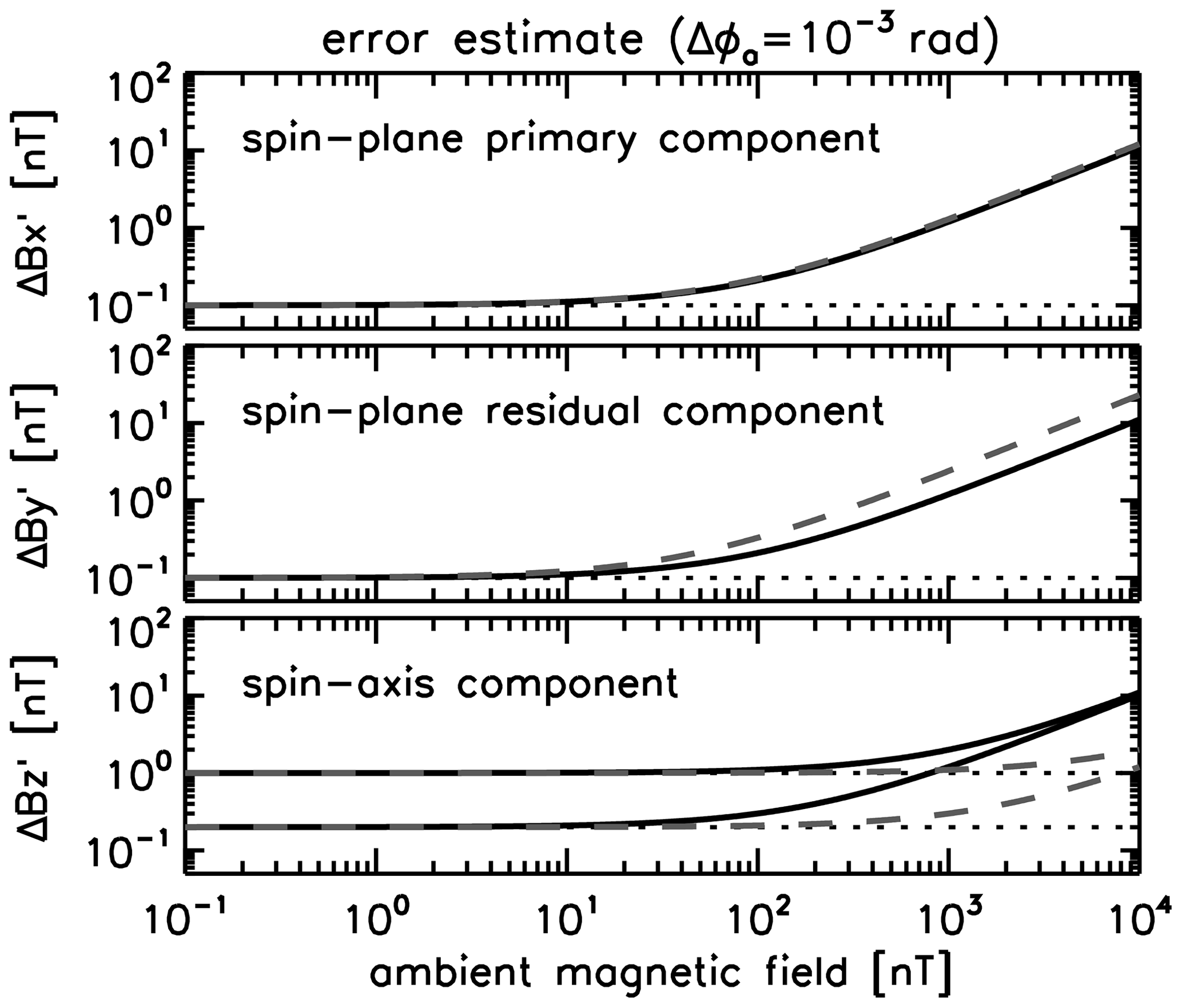
The residual component has the largest uncertainty in Fig. 2, which comes from the uncertainty of spin-plane rotation angle Δϕa. For reference purposes, Fig. 3 exhibits the combined error estimate for the error of the azimuthal angle smaller than that for Fig. 2 by an order of magnitude rad. In that case, the angle errors in the calibration parameters fall into nearly the same order (between 10−4 rad and 10−3 rad). The final error is then below 1 nT (up to an ambient field of 300 nT) even when the ambient field is along the spin axis.
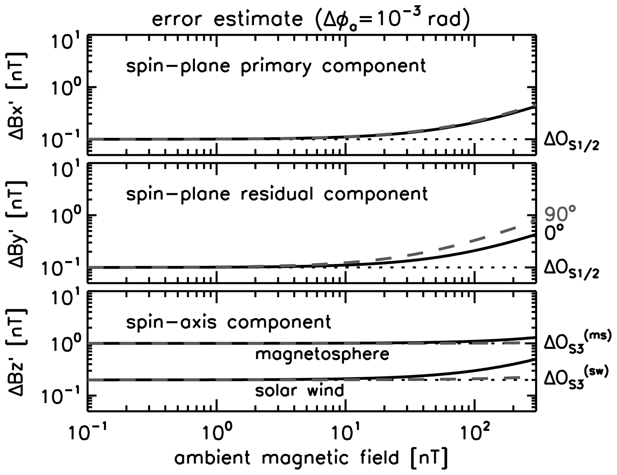
Figure 3The same plot style as Fig. 2 but for the improved error of magnetometer boom angle .
The graphical representation of the error estimates is extended to an ambient field of up to 10 000 nT and is plotted again for different values of rotation angle ( and ) in Figs. 4 and 5, respectively,
Fluxgate magnetometers are widely used in a wide range of spacecraft missions for the study of Earth's and planetary magnetospheres, solar system bodies, and the heliosphere. The magnetometer and the associated calibration process are necessarily accompanied by uncertainties that arise from various error sources. We conclude the error estimate on magnetometer in-flight calibration as follows.
-
Errors appear both as absolute ones (which are the offsets) and as relative ones (angle errors, gain errors). First-order expressions (Eqs. 33–39) (also graphically displayed in Figs. 2–5) are of practical use and show that the offset errors dominate in a low ambient field (typically below 10 nT), while the relative errors (proportional to the ambient field) dominate in a high ambient field.
-
The largest uncertainty sources are (1) the spin-axis offset error and (2) the spin-plane rotation angle error. The offset error appears as the dominant error in the low-field environment. The spin-plane rotation angle error plays a major role in a high-field environment, particularly when the ambient field is aligned in the spin plane.
The uncertainties are obtained by perturbing the calibration parameters proposed by Plaschke et al. (2019). When simplified into the first-order expression, the magnetometer data errors primarily represent the offset errors as constant and the errors of gains and angles as a relative error to the ambient field. Our derivation shows how the uncertainty sources combine through the calibration process both linearly (which is dominant) and nonlinearly through the coupling of calibration parameter errors (which is only of secondary importance when the errors of calibration parameters are small). The error formulas are presented with analytical expressions (Eqs. 33, 36, and 39) and are expected to serve as a useful tool in various applications, for example, to further minimize the final error in designing a magnetometer with a boom and verifying the error thoroughly in the ground calibration (particularly the spin-plane rotation angle) and to report the error of scientific studies which are based on magnetometer data.
It should be noted that the calibration parameters are treated as time-independent in our study. In reality, however, the calibration parameters (such as offsets and gains) depend on the temperature and can evolve along the orbit. A time-dependent picture of the calibration parameters needs an extensive in-flight calibration experience.
The errors associated with the uncertainties in calibration parameters are studied in this paper. In a low-field environment such as in interplanetary space the sensor nonlinearity (which originates in the nonlinearity of gain) is usually considered negligible. In a low Earth orbit the situation may be different. Modern sensors, which are often double wound and even triple wound, have excellent linearity (typically to an accuracy of about 10−4 per axis), but this is not always the case. The MAGSAT single-wound sensor (Acuña, 1980; Langel et al., 1982), for example, suffered from about 1 % nonlinearity, and the same sensor design was used more recently on MESSENGER (Solomon et al., 2007; Anderson et al., 2007). With the present thinking about the possibility of deploying large fleets of small-magnetometer CubeSats with just as small sensors one might ask whether nonlinearity issues can arise again.
Detailed derivative calculations in Sect. 2 are presented here.
No data sets were used in this article.
YN wrote, revised, and coordinated the work; FP, WM, DF, and DS participated in discussion and writing.
The authors declare that they have no conflict of interest.
This work was financially supported by the Austrian Space Applications Programme (ASAP) at the Austrian Research Promotion Agency under contract 865967. Yasuhito Narita also acknowledges financial support by the Japan Society for the Promotion of Science, Invitational Fellowship for Research in Japan (long term) under grant FY2019 L19527. Yasuhito Narita also thanks the research and administration staff members in the Hoshino laboratory group at the University of Tokyo for discussions, support, and organization during the fellowship program and the University of Tokyo Mejirodai International Village (MIV) for the arrangement and hospitality during the pleasant and productive stay in Tokyo.
This research has been supported by the Österreichische Forschungsförderungsgesellschaft (grant no. 865967).
This paper was edited by Valery Korepanov and reviewed by two anonymous referees.
Acuña, M. H.: The MAGSAT precision vector magnetometer, Johns Hopkins APL Technical Digest, 1, 210–213, 1980. a
Acuña, M. H.: Space-based magnetometers, Rev. Sci. Instrum., 73, 3717, https://doi.org/10.1063/1.1510570, 2002. a
Alconcel, L. N. S., Fox, P., Brown, P., Oddy, T. M., Lucek, E. L., and Carr, C. M.: An initial investigation of the long-term trends in the fluxgate magnetometer (FGM) calibration parameters on the four Cluster spacecraft, Geosci. Instrum. Method. Data Syst., 3, 95–109, https://doi.org/10.5194/gi-3-95-2014, 2014. a, b, c
Anderson, B. J., Acuña, M. H., Lohr, D. A., Scheifele, J., Raval, A., Korth, H., and Slavin, J. A.: The magnetometer instrument on MESSENGER, Space Sci. Rev., 131, 417–450, https://doi.org/10.1007/s11214-007-9246-7, 2007. a
Angelopoulos, V.: The THEMIS mission, Space Sci. Rev., 141, 5, https://doi.org/10.1007/s11214-008-9336-1, 2008. a
Auster, H. U., Glassmeier, K. H., Magnes, W., Aydogar, O., Baumjohann, W., Constantinescu, D., Fischer, D., Fornacon, K. H., Georgescu, E., Harvey, P., Hillenmaier, O., Kroth, R., Ludlam, M., Narita, Y., Nakamura, R. Okrafka, K., Plaschke, F., Richter, I., Schwarzl, H., Stoll, B., Valavanoglou, A. and Wiedemann, M.: The THEMIS Fluxgate Magnetometer, Space Sci. Rev., 141, 235–264, https://doi.org/10.1007/s11214-008-9365-9, 2008. a
Balogh, A., Carr, C. M., Acuña, M. H., Dunlop, M. W., Beek, T. J., Brown, P., Fornacon, K.-H., Georgescu, E., Glassmeier, K.-H., Harris, J., Musmann, G., Oddy, T., and Schwingenschuh, K.: The Cluster Magnetic Field Investigation: overview of in-flight performance and initial results, Ann. Geophys., 19, 1207–1217, https://doi.org/10.5194/angeo-19-1207-2001, 2001. a
Burch, J. L., Moore, T. E., Torbert, R. B., and Giles, B. L.: Magnetospheric Multiscale overview and science objectives, Space Sci. Rev., 199, 5–21, https://doi.org/10.1007/s11214-015-0164-9, 2016. a
Escoubet, C. P., Fehringer, M., and Goldstein, M.: Introduction The Cluster mission, Ann. Geophys., 19, 1197–1200, https://doi.org/10.5194/angeo-19-1197-2001, 2001. a
Frühauff, D., Plaschke, F., and Glassmeier, K.-H.: Spin axis offset calibration on THEMIS using mirror modes, Ann. Geophys., 35, 117–121, https://doi.org/10.5194/angeo-35-117-2017, 2017. a, b, c, d
Goetz, C., Koenders, C., Hansen, K. C., Burch, J., Carr, C., Eriksson, A., Frühauff, D., Güttler, C., Henri, P., Nilsson, H., Richter, I., Rubin, M., Sierks, H., Tsurutani, B., Volwerk, M., and Glassmeier, K. H.: Structure and evolution of the diamagnetic cavity at comet 67P/Churyumov-Gerasimenko, Mon. Not. R. Astron. Soc., 462, S459–S467, https://doi.org/10.1093/mnras/stw3148, 2016a. a
Goetz, C., Koenders, C., Richter, I., Altwegg, K., Burch, J., Carr, C., Cupido, E., Eriksson, A., Güttler, C., Henri, P., Mokashi, P., Nemeth, Z., Nilsson, H., Rubin, M., Sierks, H., Tsurutani, B., Vallat, C., Volwerk, M., and Glassmeier, K.-H.: First detection of a diamagnetic cavity at comet 67P/Churyumov-Gerasimenko, Astron. Astrophys., 588, A24, https://doi.org/10.1051/0004-6361/201527728, 2016b. a
Hedgecock, P. C.: A correlation technique for magnetometer zero level determination, Space Sci. Instrum., 1, 83–90, 1975. a
Kepko, E. L., Khurana, K. K., Kivelson, M. G., Elphic, R. C., and Russell, C. T.: Accurate determination of magnetic field gradients from four point vector measurements. I. Use of natural constraints on vector data obtained from a single spinning spacecraft, IEEE T. Magnet., 32, 377–385, https://doi.org/10.1109/20.486522, 1996. a, b
Langel R., Ousley G., Berbert J., Murphy J., and Settle M.: The MAGSAT Mission. Geophys. Res. Lett., 9, 243–245, https://doi.org/10.1029/GL009i004p00243, 1982. a
Leinweber, H. K., Russell, C. T., Torkar, K., Zhang, T. L., and Angelopoulos, V.: An advanced approach to finding magnetometer zero levels in the interplanetary magnetic field, Meas. Sci. Technol., 19, 055104, https://doi.org/10.1088/0957-0233/19/5/055104, 2008. a
Nakamura, R., Plaschke, F., Teubenbacher, R., Giner, L., Baumjohann, W., Magnes, W., Steller, M., Torbert, R. B., Vaith, H., Chutter, M., Fornaçon, K.-H., Glassmeier, K.-H., and Carr, C.: Interinstrument calibration using magnetic field data from the flux-gate magnetometer (FGM) and electron drift instrument (EDI) onboard Cluster, Geosci. Instrum. Method. Data Syst., 3, 1–11, https://doi.org/10.5194/gi-3-1-2014, 2014. a
Plaschke, F., Nakamura, R., Leinweber, H. K., Chutter, M., Vaith, H., Baumjohann, W., Steller, M., and Magnes, W.: Fluxgate magnetometer spin axis offset calibration using the electron drift instrument, Meas. Sci. Technol., 25, 105008, https://doi.org/10.1088/0957-0233/25/10/105008, 2014. a
Plaschke, F. and Narita, Y.: On determining fluxgate magnetometer spin axis offsets from mirror mode observations, Ann. Geophys., 34, 759–766, https://doi.org/10.5194/angeo-34-759-2016, 2016. a, b
Plaschke, F., Goetz, C., Volwerk, M., Richter, I., Frühauff, D., Narita, Y., Glassmeier, K.-H., and Dougherty, M. K.: Fluxgate magnetometer offset vector determination by the 3D mirror mode method, Mon. Not. R. Astron. Soc., 469, S675–S684, https://doi.org/10.1093/mnras/stx2532, 2017. a
Plaschke, F., Auster, H.-U., Fischer, D., Fornaçon, K.-H., Magnes, W., Richter, I., Constantinescu, D., and Narita, Y.: Advanced calibration of magnetometers on spin-stabilized spacecraft based on parameter decoupling, Geosci. Instrum. Method. Data Syst., 8, 63–76, https://doi.org/10.5194/gi-8-63-2019, 2019a. a, b, c, d, e, f, g, h, i, j, k, l, m, n, o, p
Plaschke, F.: How many solar wind data are sufficient for accurate fluxgate magnetometer offset determinations?, Geosci. Instrum. Method. Data Syst., 8, 285–291, https://doi.org/10.5194/gi-8-285-2019, 2019b. a, b, c
Russell, C. T., Anderson, B. J., Baumjohann, W., Bromund, K. R., Dearborn, D., Fischer, D., Le, G., Leinweber, H. K., Leneman, D., Magnes, W., Means, J. D., Moldwin, M. B., Nakamura, R., Pierce, D., Plaschke, F., Rowe, K. M., Slavin, J. A., Strangeway, R. J., Torbert, R., Hagen, C., Jernej, I., Valavanoglou, A., and Richter, I.: The Magnetospheric Multiscale Magnetometers, Space Sci. Rev., 199, 189–256, https://doi.org/10.1007/s11214-014-0057-3, 2016. a
Schmid, D., Plaschke, F., Narita, Y., Heyner, D., Mieth, J. Z. D., Anderson, B. J., Volwerk, M., Matsuoka, A., and Baumjohann, W.: Magnetometer in-flight offset accuracy for the BepiColombo spacecraft, Ann. Geophys., 38, 823–832, https://doi.org/10.5194/angeo-38-823-2020, 2020. a, b
Solomon, S. C., McNutt Jr., R. L., Gold, R. E., Domingue, D. L.: MESSENGER mission overview, Space Sci. Rev., 131, 3–39, https://doi.org/10.1007/s11214-007-9247-6, 2007. a
- Abstract
- Introduction
- Systematic error on in-flight calibration
- Estimate of calibration parameter errors
- Combined errors of calibrated magnetometer data
- Conclusions
- Appendix A: Derivatives
- Data availability
- Author contributions
- Competing interests
- Acknowledgements
- Financial support
- Review statement
- References