the Creative Commons Attribution 4.0 License.
the Creative Commons Attribution 4.0 License.
 | 18 Aug 2021
Production of definitive data from Indonesian geomagnetic observatories
Relly Margiono
Christopher W. Turbitt
Ciarán D. Beggan
Kathryn A. Whaler
Measurement of the geomagnetic field in Indonesia is undertaken by the Meteorological, Climatological, and Geophysical Agency (BMKG). Routine activities at each observatory include the determination of declination, inclination, and total field using absolute and variation measurements. The oldest observatory is Tangerang (TNG), started in 1957, followed by Tuntungan (TUN) in 1980, Tondano (TND) in 1990, Pelabuhan Ratu (PLR) and Kupang (KPG) in 2000, and Jayapura (JAY) in 2012. One of the main obligations of a geomagnetic observatory is to produce final versions of data, released as definitive data, for each year and make them widely available both for scientific and non-scientific purposes, for example to the World Data Centre of Geomagnetism (WDC-G). Unfortunately, some Indonesian geomagnetic observatories do not share their data with the WDC-G and often have difficulty in producing definitive data. In addition, some more basic problems still exist, such as low-quality data due to anthropogenic or instrumental noise, a lack of data-processing knowledge, and limited observer training. In this study, we report on the production of definitive data from Indonesian observatories, and some recommendations are provided about how to improve the data quality. These methods and approaches are applicable to other institutes seeking to enhance their data quality and scientific utility, for example in main field modelling or space weather monitoring. The definitive data from the years 2010 to 2018 are now available in the WDC-G.
- Article
(6772 KB) - Full-text XML
- BibTeX
- EndNote


A geomagnetic observatory is a permanent site or installation at which the geomagnetic field vector and strength is continuously recorded as a function of time at the Earth's surface. The main objective of an observatory is to record the change of geomagnetic field over both short (e.g. daily variation, magnetic storms) and long (e.g. secular variation) periods. Unfortunately, the spatial distribution of geomagnetic observatories is uneven, and they are concentrated in the Northern Hemisphere (Rasson et al., 2011). Although recent satellite missions such as CHAMP and Swarm (Friis-Christensen et al., 2006; Reigber et al., 2002) have extended global coverage of the magnetic field, there is no guarantee that satellites will continue to operate over an extended period. In addition, satellite measurements are affected by ionospheric current systems and are subject to time–space ambiguity. Therefore, installing and maintaining ground observatories is a sensible way to guarantee the continuity of magnetic data records.
In order to reach high-quality levels of geomagnetic data useful for scientific purposes, it is generally necessary to adhere to standards, for example those defined by INTERMAGNET (St-Louis, 2012), an international body whose members agree to a set of defined rules and metrics for the consistent operation of observatories. Not all geomagnetic observatories are part of this network, as there are minimum requirements in terms of the type and quality of observatory instrumentation, data processing, and transmission. Currently there are around 130 INTERMAGNET observatories, but again the spatial distribution is still weighted to the European and North American sectors. It is obligatory for each observatory to send their final definitive data once per year, though they also can provide data after preliminary processing, which are referred to as quasi-definitive (QD) data (Clarke et al., 2013; Peltier and Chulliat, 2010). In addition, INTERMAGNET also allows observatories to send their data in near real time through Geomagnetic Information Nodes (GINs). Note that these near-real-time data are not definitive either but can be useful for purposes such as space weather applications. Observatories that do not reach INTERMAGNET standards can alternatively provide their data to the World Data Centre of Geomagnetism (WDC-G). However, the data should be definitive.
Indonesia has six geomagnetic observatories, which are operated by the Meteorological Climatological and Geophysical Agency (BMKG). Unfortunately, the data quality is often poor, due to noise in the measurements and poor data processing techniques. In addition, there is a tendency for slow transmission of the data, and thus no observatory has joined the INTERMAGNET network yet. There is also a lack of Indonesian observatory data in the WDC-G, which means geomagnetic data in this region cannot be fully utilised. This is particularly unfortunate as the equatorial regions display magnetic field features, such as the Equatorial Electrojet (EEJ) (Sugiura and Cain, 1966), and currently exhibit rapid secular variation and acceleration (Kloss and Finlay, 2019). For these reasons, we have made considerable efforts to create definitive data from Indonesian observatories and store them in the WDC-G data portal. This paper reports the work undertaken to produce definitive data from Indonesian observatories and provides recommendations for improvement. In addition, we offer it as a template for other institutes wishing to identify issues and improve the quality of data from their observatory network.
We utilised data from four Indonesian observatories, Tuntungan (TUN), Pelabuhan Ratu (PLR), Tondano (TND), and Kupang (KPG); their locations are given in Table 1, and a map of the observatories is displayed in Fig. 1. The data consist of raw magnetic measurements from variometers and scalar instruments, as well as absolute observations. For modern geomagnetic observatories, two types of observation are made that consist of absolute measurements and relative measurements or variations. An absolute measurement is a manual observation to determine the true strength and direction of the magnetic field vector in the geographic reference frame at a particular time (typically only once or twice per week) using an absolute magnetometer (e.g. declination inclination magnetometer, proton precession magnetometer), whereas relative measurements are continuous observations (usually once per second) of the variations in the field vector using an automatically recorded variometer (e.g. a Fluxgate magnetometer). This type of instrument is installed on a stable pillar to reduce the effect of movement or drift over time.
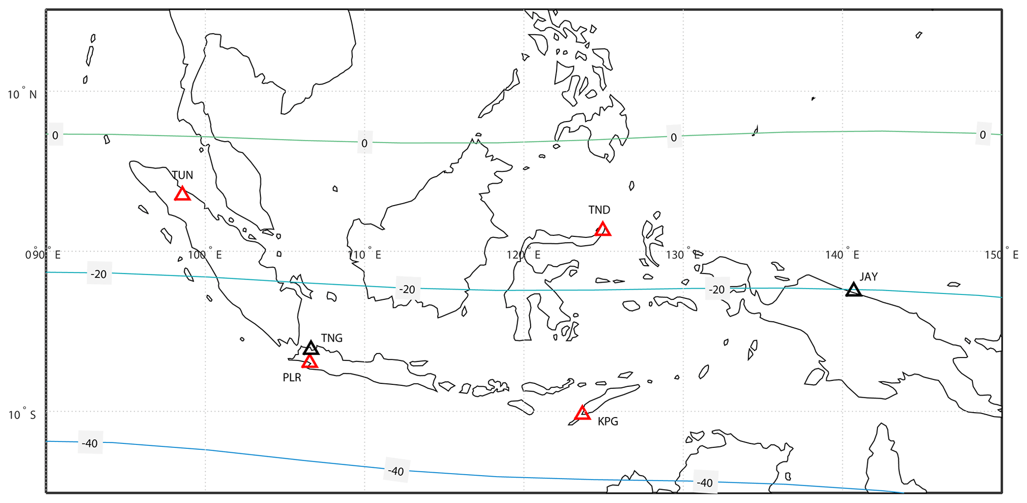
Figure 1Indonesian geomagnetic observatory map. The red triangles are observatories from which data are used in this paper. The black triangles are observatories from which data are not used in this paper. The IAGA codes are depicted by the three-letter names of each observatory (JAY is still a provisional code). The contours are of the inclination of magnetic field in degrees from the 2015 WMM (World Magnetic Model) (Chulliat et al., 2015).
Table 1Indonesian observatories which are used to derive definitive data.

Measurements in Indonesia are a combination of several instruments of different type and age depending on the observatory in question. Note that due to the large size of the country, the observatories operate as semi-independent services that provide data to BMKG as the central hub and funder. As part of the study we wished (a) to understand the data issues at each of the observatories and (b) to produce a revised set of magnetic field measurements that are as close to definitive data as possible. In order to do this, we asked for the raw magnetic data from the observatories by means of an individual direct request. Once we had collected the raw data, depending on the availability of both variation and absolute data (see Table 1), we began to examine each dataset to identify the root causes of any issues and prepare a processing chain to produce definitive data.
Definitive data production
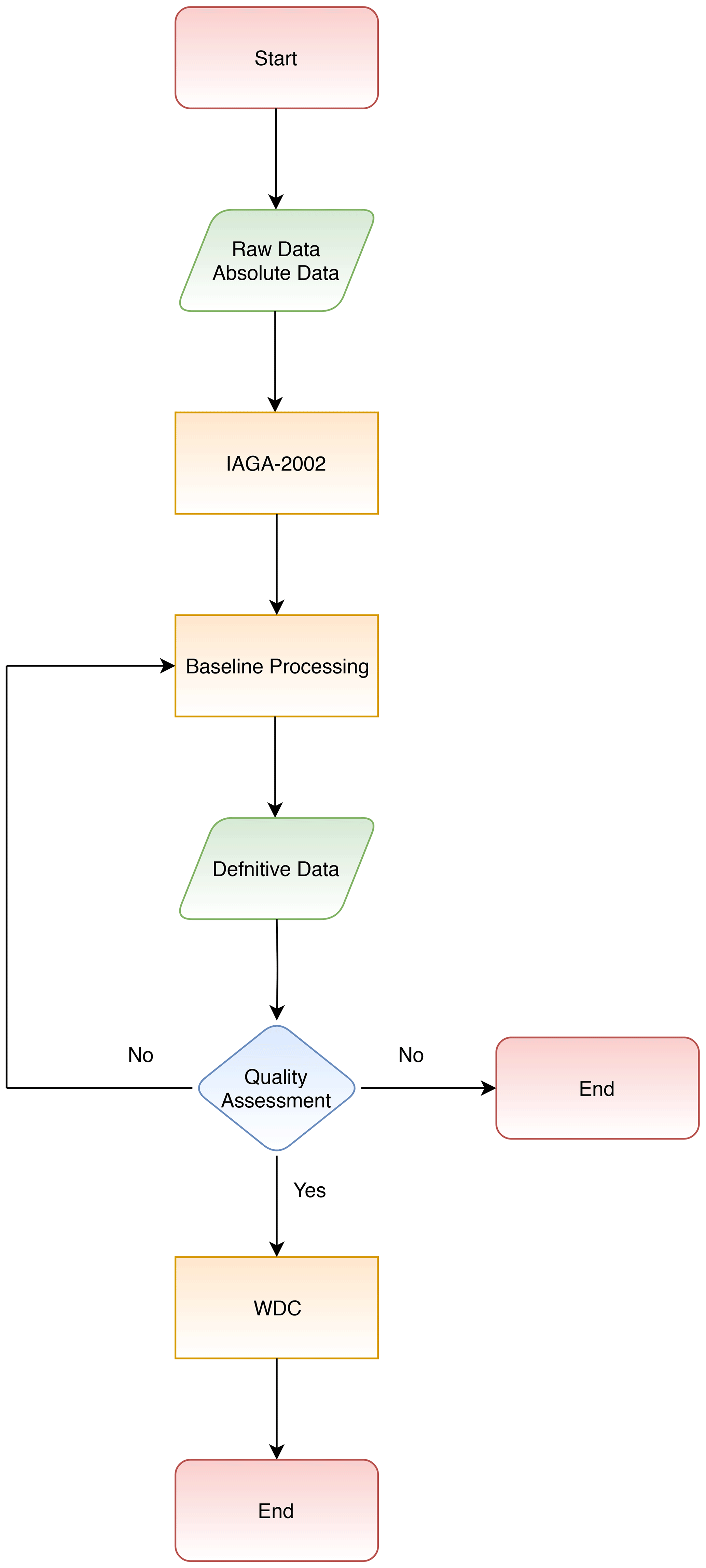
Figure 2 shows a flowchart of the definitive data processing steps we adopted. Producing definitive data begins by collecting absolute and variometer raw data, as seen in Table 1. We note that each observatory has a different sampling rate depending on the instruments deployed (e.g. 1 s, 5 s). We initially tried to produce variation data using the 1 min IAGA-2002 format (https://www.ngdc.noaa.gov/IAGA/vdat/IAGA2002/iaga2002format.html, last access: 10 August 2021) as the standard data format by applying the Gaussian filters recommended by INTERMAGNET. We also checked the raw variometer data prior to the conversion to the standard format to assess whether or not the raw data were noisy (i.e. containing unwanted, artificial signal); any noisy data were removed following the method of Khomutov et al. (2017). Normally, each observatory has a single data logger to capture the variometer and scalar proton data; however, if the loggers are separate, we performed additional processing to ensure that both datasets are correctly combined (e.g. aligning by timestamp).
The next stage, baseline calculation, is an important part of the processing, and the stability of the result determines the absolute accuracy of the processed data. Inaccuracy in the processing will affect the final definitive data released. To provide an accurate calculation, first we should understand the orientation of the variometer sensor. The HEZ (magnetic north, magnetic east, vertically downwards) orientation is the most popular at a magnetic observatory due to the ease of the installation, i.e. it only requires orienting one of the horizontal sensors to the magnetic east direction (indicated by a zero value in the output of the E sensor) so that the orthogonal sensor is directly pointing to magnetic north. In contrast, some researchers argue that the geographic XYZ (north, east, vertically downwards) orientation will produce a more stable installation because the sensor does not need a readjustment in the future and is very suitable for observatories that are located at high latitudes (Jankowski and Suckdorff, 1996). However, installation in the XYZ direction needs proper initial measurement to determine the geographic north (X) or geographic east (Y) direction prior to the installation, and observatories can unintentionally introduce errors during the installation stage should the sensors be installed with some alignment errors (Rasson, 2005). However, Gonsette et al. (2017) show it is possible to determine a baseline from all types of sensor orientation using correction methods even with a non-ideal installation (e.g. an unstable pillar). Their method needs a high frequency of absolute measurements, which can be made using an automatic observatory (Poncelet et al., 2017) but might be difficult to apply at a normal observatory. In this paper, we will describe how we determined an instantaneous baseline from the HEZ sensor orientation.
The definition of the magnetic field vector and of the magnetometer sensor orientation often leads to confusion because the magnetometer can be oriented in a different position (HEZ, XYZ, DFI) to the field vector. After installation, the magnetometer remains static, but the vector field changes over time. Here, we describe the three orthogonal magnetometer sensors of the fluxgate as P, Q, and Z (Fig. 3). In this description, both the vertical downward magnetic field vector and vertical component sensor (Z) are the same.
A fluxgate magnetometer only measures a relative variation of the magnetic field. These variation data must be corrected with an offset value in three components, commonly known as the instrument baselines, which includes terms accounting for the bias field applied to the sensor, electronic offsets, and gradients in the magnetic field vector between the variometer position and the absolute measurement position (Turbitt, 2003). Where a continuously recording scalar instrument (such as a proton precession magnetometer or PPM) is also being operated, a similar baseline measurement, known as a site difference, is applied to account for field gradients between the scalar instrument and the absolute measurement position. The site difference can be evaluated by temporarily running a secondary scalar instrument at the absolute measurement position. This value is then used both as a quality reference for the variometer data and in the process of determining the field vector at the absolute measurement position during manual measurements.
Typically, a manual absolute measurement resolves the time-varying field vector in the spherical components set defined as declination (DA(t)), inclination (IA(t)), and total field (FA(t)). Other commonly used components (e.g. HA(t) and ZA(t)) can be derived using Eqs. (1) and (2). The absolute values for D and I are typically computed from the average of four measurements made with a fluxgate magnetometer attached to a non-magnetic theodolite. Details of how to make the absolute observations and the recommended procedure can be found in Jankowski and Suckdorff (1996), Rasson (2005), and Turbitt (2003).
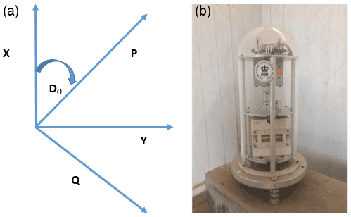
Figure 3Sensor orientation (a) of a typical fluxgate magnetometer (b) in the horizontal plane. P and Q define the orthogonal sensors aligned in the horizontal plane, Do is the declination, and X and Y are geographic north and east.
Details of baseline calculation for each component (vertical, horizontal and declination components) are given in Appendix A.
Finally, data quality assessment is performed. In this paper, we will focus on presenting the data quality by measuring ΔF, as this value can describe the quality of recording (Reda et al., 2011). The ΔF value is the difference between the total field calculated from the fluxgate (Fcal) and scalar proton (Fsc) magnetometers. This value, which should be a straight line, is significant for checking the quality of a recording. Spikes in ΔF are commonly detected due to an internal or external problem such as fluxgate electronic failure or a car parked near the variometer building. The length of the spike corresponds to the length of the perturbation. When the source of the perturbation is removed, the spike will also disappear. Jumps or long-term drift in ΔF indicate a problem in the baseline. When the ΔF plot is similar to the variation data, it can be concluded that there is a problem in the scale value. The scale value is a scale to convert the fluxgate output from volts to nanoteslas (nT). In addition, we will also analyse the temperature of both the fluxgate electronics and fluxgate sensor. The fluxgate sensor is temperature dependent, and an unstable temperature will undermine the quality of the recording (Reda et al., 2011).
Figure 4 shows definitive data for four Indonesian magnetic observatories (TUN, KPG, TND, PLR). Note that the Jayapura (JAY) and Tangerang (TNG) observatories have not been included in the results as their data quality was not good enough to be added to the WDC-G. In the case of TNG, the data have problems due to numerous spikes and steps (Fig. 5a). This noise is assumed to be associated with electric trains that operate in Tangerang City. The railway, installed in 1997, runs less than 1 km from the observatory. Consequently, the electrical current from the train leaks into the ground and interferes with the geomagnetic data (Pirjola, 2011; Curto et al., 2008). Jankowski and Suckdorff (1996) stated that a geomagnetic observatory should be at least 300 m from other buildings and 1 km from a railway. If the train system is electric, the distance should be several kilometres (tens of kilometres for DC trains). For this reason, we can conclude that the location of TNG is no longer suitable for recording geomagnetic activity. However, TNG's night-time data are potentially usable, as in this period trains are not running, meaning that the data are quieter than during the day. JAY is a new observatory and thus is not included due to insufficient data being available at present from this station.
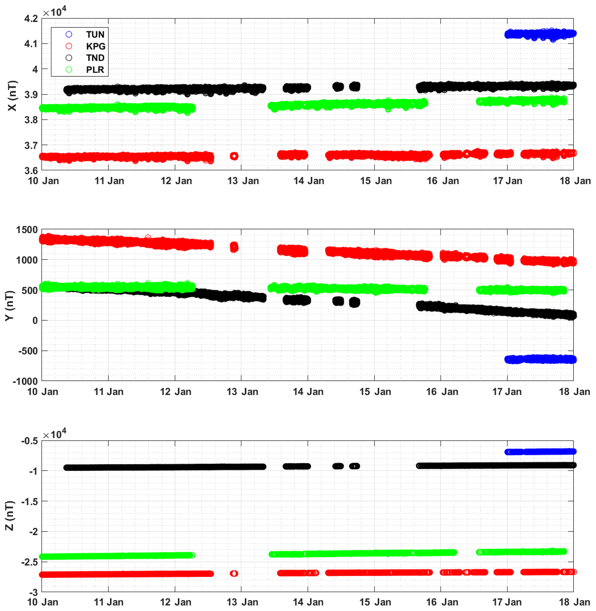
Figure 4Hourly means at Indonesian observatories in the WDC-G data portal for the period 2010–2017.
Figure 4 shows that from the beginning of 2010, all observatories generally have excellent data continuity, but from 2012 onward gaps appear in their records. The INDIGO project, which helps to build new observatories and supports the existing observatories in Indonesia, was launched in early 2010. This project gave digitisers and magnetometers to the Indonesian observatories under coordination of the British Geological Survey (BGS) and Institut Royal Météorologique de Belgique (IRM) (Rasson et al., 2011). A couple of years after this project was initiated, problems such as sensor and digitiser faults arose. In addition, the local operators do not have the ability to fix the instrument themselves, instead returning the instrument to the UK to be repaired, delaying their return to service. The broken instruments meant the complete observation of magnetic fields could not be carried out, and this impacted the quantity of data available.
Starting in 2016, BMKG initiated a project to standardize the sampling rate of fluxgate data recording. The institution preferred to have a faster sampling rate (e.g. 1 s) as BMKG wishes to detect magnetic anomalies perhaps associated with events, e.g. earthquake precursors (Ahadi et al., 2015). BMKG also required all observatories to use the LEMI format (Lviv, 2008) as standard, and thus the old (INDIGO) format was replaced. The change of data format resulted in a new problem as the LEMI format gives a pseudo-offset in the fluxgate data. This offset produced discontinuities in the baseline record. Consequently, some observatories have had to adjust their baseline calculation to produce the correct baseline. In addition, other problems such as timing inaccuracies between fluxgate sensors and scalar proton magnetometers arose because the new systems were not recording to a single data logger, as was the case with INDIGO equipment. Thus, the observers needed to manually fix these issues if timing discrepancies occurred.
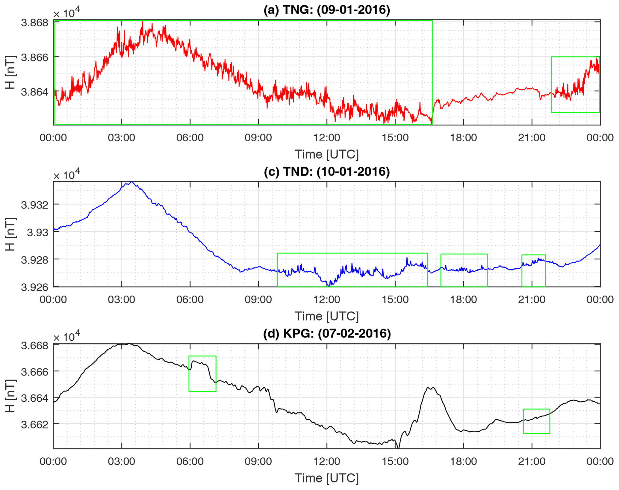
Figure 5Example artificial disturbance (or “noise”) in Indonesian observatory data during 2016. Data are the computed minute-mean values. The green boxes indicate the periods of disturbance.

Figure 6Histogram of rate of change and step periods at KPG observatory. Panels (a), (b), and (c) are histograms of the rate of change in the H, E, and Z components, respectively, and (d) is the step period. Magenta lines in the histograms of the rate of change are the assumed step threshold.
At some of the observatories, gaps after 2016 are due to the occurrence of noise in the data. This noise was identified as random noise at TNG (Fig. 5a) and TND (Fig. 5b) and steps in KPG (Fig. 5c). We found that the random noise at TND and TNG was difficult to treat, and the best way of dealing with it was to delete the noisy segments (Khomutov et al., 2017), consequently producing large gaps of missing data.
Removing the step noise at KPG is difficult as the magnitude of the steps varies every day and there is no fixed pattern, meaning that automatic detection via an algorithm is not possible. We constructed histograms of the first differences or rates of change for each component (, , and ) for a year of minute-mean variations of KPG data and assumed that absolute rates of change > 0.5 nT/min were most likely steps created by artificial disturbance rather than natural field variations (Fig. 6a, b and c). From Fig. 6a–c, we can see that the rate of change follows a Laplacian distribution and that the majority of the rates of change are within the step threshold. The step durations in the minute-mean variation data were estimated by eye (Fig. 6d) as the steps vary in amplitude (which is why they are difficult to detect automatically). We can see (Fig. 6d) that the duration of a step is typically less than 1 h (the histogram is binned every 60 min), from which we can conclude that filtering the data with a span of 1 h or less will not attenuate the effect of these artificial signals from the time series; i.e. the steps will be evident in 1 min and hourly mean values. However, the symmetrical distribution of these disturbances and their relatively short duration mean that we are able filter out these steps by means of daily mean values.
Regarding the assessment of the data quality, we plot ΔF for the individual variometers of the observatories in Fig. 7. The plots are divided into two categories: daily mean and daily range of ΔF. The daily means of ΔF are close to zero, and the daily ranges of ΔF are below 2 nT. From these plots we can conclude that the data quality is good enough from all observatories.
The temperature analysis is depicted in Fig. 8. Indonesia is a tropical country that only has two seasons in a year (rainy and dry season), and the average temperature is 28 ∘C (https://en.wikipedia.org/wiki/Climate_of_Indonesia, last access: 10 August 2021). The temperature difference between day and night is not too wide, but in terms of geomagnetic data quality, the temperature in the variometer building should remain constant. From Fig. 8, it is obvious that the daily and monthly temperature prior to 2017 shows a wide range, especially for PLR and KPG. This means that the variometer buildings were not set up properly and the buildings were not temperature insulated. In mid-2016 for PLR and early 2017 for KPG, the daily and monthly temperature range were better. In addition, the temperature range for TND remains steady from 2010 to 2017. In Appendix B, we add a new recommendation for BMKG to maintain the stability of temperature in the variometer buildings because it can affect the data quality.
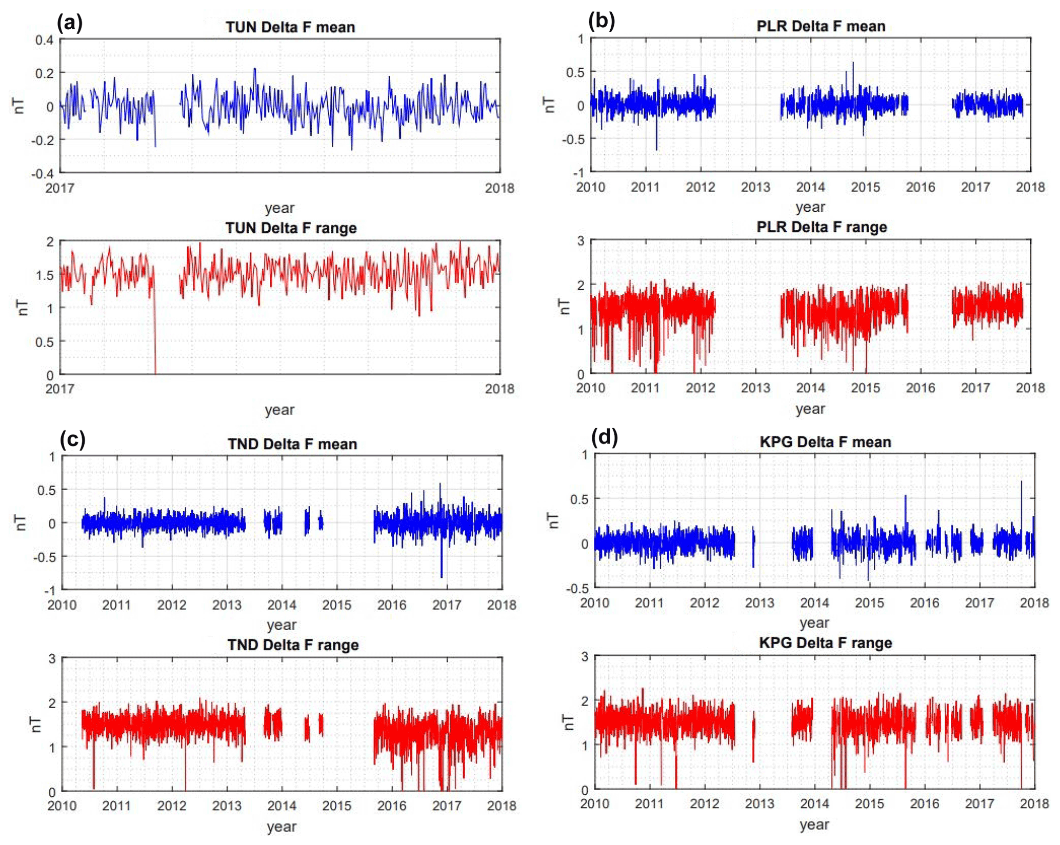
Figure 7Daily mean (blue lines) and daily range (red lines) of the ΔF plot from four Indonesian observatories. The panels show data from (a) TUN, (b) PLR, (c) TND, and (d) KPG.
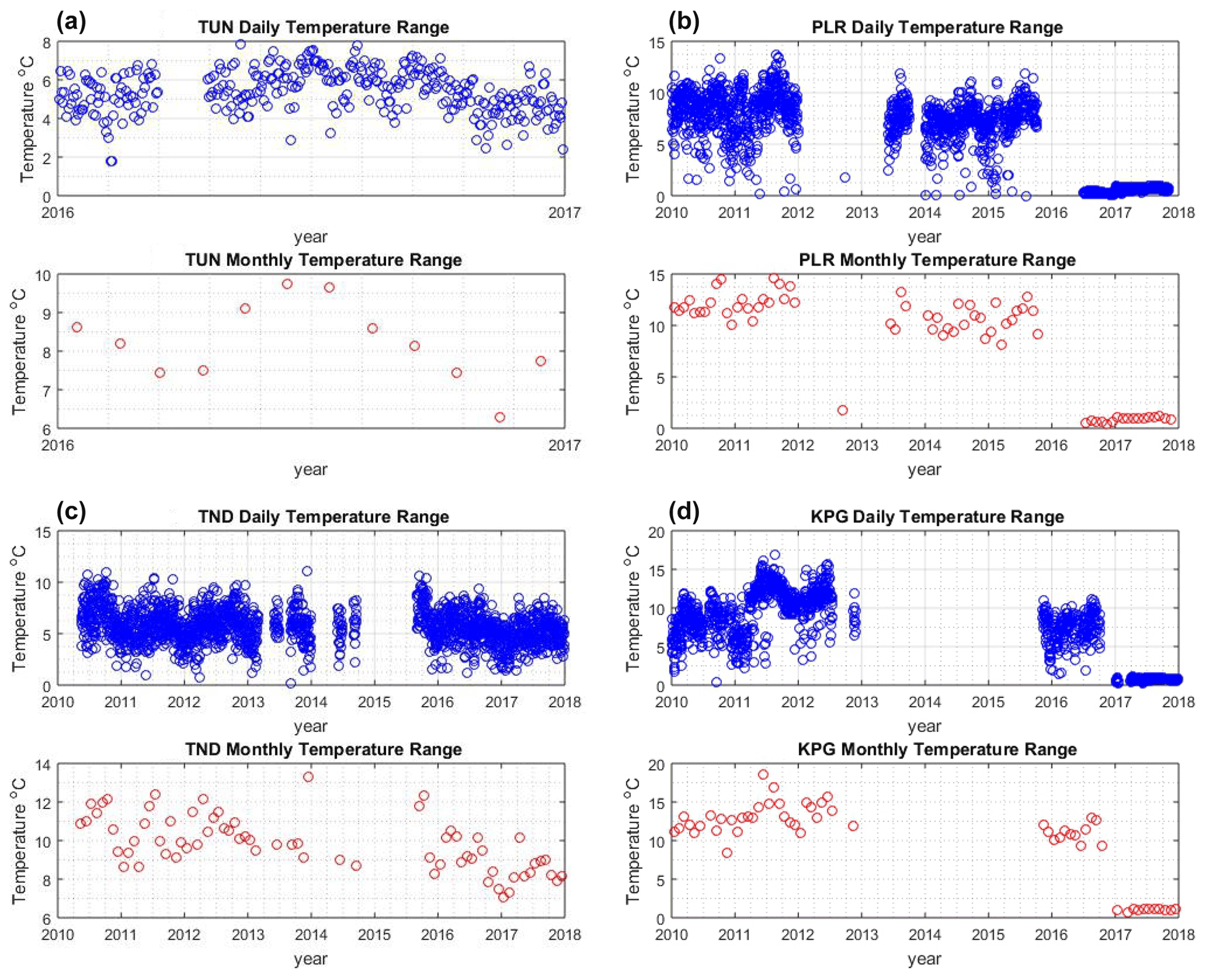
Figure 8Daily range (blue circle) and monthly range (red circle) of temperature from four Indonesian observatories. The panels show data from (a) TUN, (b) PLR, (c) TND, and (d) KPG.
To measure how well the Indonesian observatory data monitor secular variation, we compared the data to the main field model CHAOS-6 (Finlay et al., 2016) as seen in Fig. 9. The secular variation is computed using annual differences of monthly means. From Fig. 9, we can see that the vertical component secular variation (in nT/year) has an increasing and decreasing pattern. KPG secular variation matches the overall trend of the CHAOS-6 model, as does KDU as reference. PLR shows a trend similar to the CHAOS-6 model, but this is dominated by large variations in the secular variation values, which are also present in the TND data, and are characterised by bigger RMS differences from CHAOS-6. This large variation is possibly due to the presence of an external magnetic field signal such as the Equatorial Electrojet (EEJ). If this is the case, further processing would be required to isolate secular variation from the PLR and TND data, such as the proxy method (Cox et al., 2018; Brown et al., 2013). Isolating the secular variation could yield signals such as geomagnetic jerks (Brown et al., 2013), for which there is a lack of data in the Indonesian region.
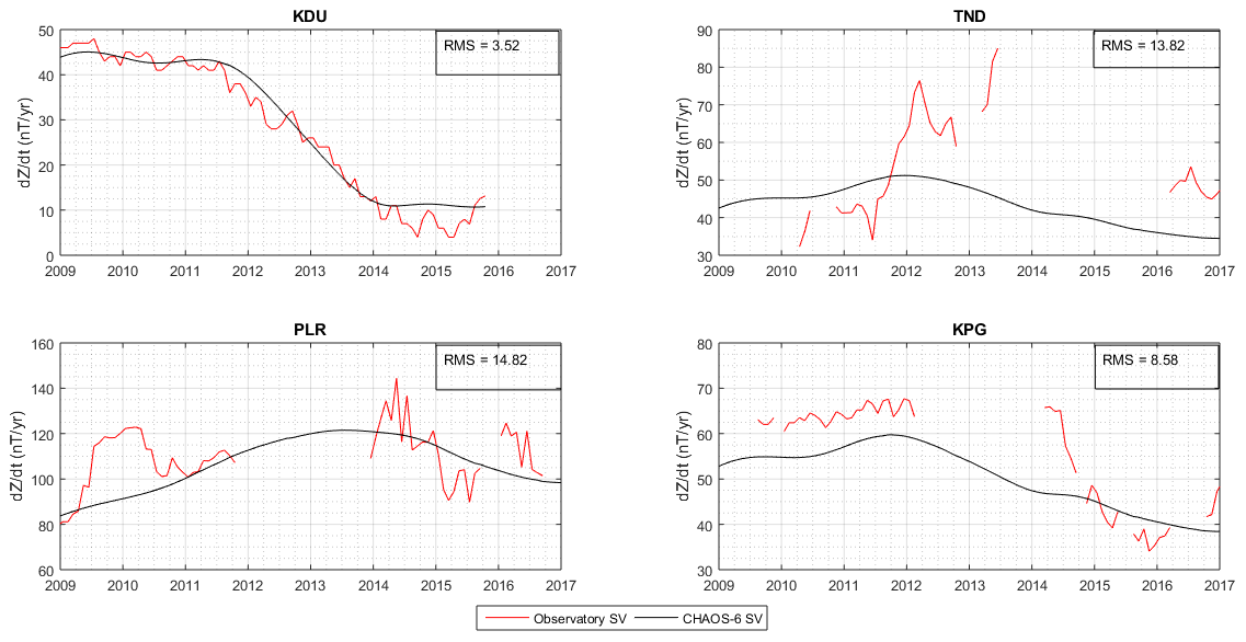
Figure 9Secular variation comparison between Indonesian Observatory Data (KPG, PLR and TND) and CHAOS-6 model (Finlay et al., 2016). Kakadu (KDU) is included as a reference observatory near to Indonesia. The secular variation is computed using annual difference of monthly means. RMS values indicate the difference from CHAOS-6 in nT/year.
In Sect. 2, some methods to improve geomagnetic data quality are described. We have applied those methods to assess Indonesian data quality and found that each observatory has its own specific problems; for each we recommended some improvements that were implemented to enhance the data quality. However, issues related to making the absolute observations and data processing remain. The major problem we found was in producing definitive data as a final step in the geomagnetic processing chain. Before this study began, there was a lack of Indonesian definitive data in the WDC portal. Consequently, Indonesian observatory data could not be used for applications such as geomagnetic modelling (e.g. McLean et al., 2004; Gillet et al., 2015).
Absolute geomagnetic observations at the magnetic observatory require proper care and attention. For absolute observations, the role of the observer is a vital consideration in order to produce high-quality data. An observer needs suitable knowledge about the technical aspects of absolute measurement, and an adequate understanding of the science of the magnetic field is also necessary. We found that some observers at Indonesian observatories only focused on the technical aspects, regardless of the fundamental science, causing mistakes to be made. For example, some of them still had magnetic materials on them while performing absolute observations (e.g. mobile phones or jewellery); in fact, these materials clearly contributed to measurement errors. The only way to make better absolute measurements is by considering all aspects both technical and practical and improving the operator skill level; subsequently, a series of workshops and seminars were organised to educate and inform the observers and encourage them to raise their own standards.
Variation measurements are the other form of observation at an observatory. These observations mainly depend on the performance of the automated instruments that measure the magnetic field continuously. The basic requirement to achieve excellent recording is to locate the sensor at a quiet place so that it only measures the natural magnetic field. Some Indonesian geomagnetic observatories are not located in ideal places, and this problem will only be overcome by moving the observatory to a better location with initial and proper site surveying prior to installation. In addition, the sensor orientation and related installation techniques have to be considered. A poor installation can have an impact on baseline processing and ultimately on the absolute accuracy of the published definitive data. The HEZ orientation is popular in our observatories as this is easy to install and (as shown) the derivation of its instrument baselines is relatively straightforward. However, one observatory does use the XYZ orientation, which is more challenging to process as any error in installation is difficult to compensate for in post-processing.
Geomagnetic data processing is the next stage after absolute and variation observations are performed. The primary sources for this processing are raw data from absolute and variation observation. These raw data are then processed to produce final definitive data. We found that Indonesian observatories did not use standard processing tools. At some observatories, data processing relied on manual processing assisted by use of a computer spreadsheet, while others had established their own data processing using tools written in common programming languages. The lack of a data processing standard made the final definitive data production difficult, especially for the observatories that still use manual calculation. Although they produced daily means, monthly means, and annual means, the data format was not standardised. As manual processing is slow, it cannot handle more challenging tasks such as data conversion, data merging, and transmission. To remedy this, we introduced a user-friendly software, namely GDASview (http://www.geomag.bgs.ac.uk/code/GdasView/launch.html, last access: 10 August 2021), developed by the British Geological Survey, to help automate data processing at Indonesian observatories.
Finally, the data from four Indonesian observatories are now available at the WDC data portal. These definitive data still have limitations such as data gaps and less accurate baselines, but the quality is reasonable enough to be made available to the international community. The justification for this is based on visual analysis, data quality checks, and the implementation of a standardised method to produce definitive data. We hope the data quality will improve and that all of the Indonesian observatories will obtain INTERMAGNET certification in the near future. In addition, robust data quality measurements that include more numerical calculation are recommended, such as using momentary values (Curto and Marsal, 2007) or a more statistical approach (Zhang et al., 2016), but both methods rely on complete data series. This should be accomplished in the next few years. We expect that this work will have an impact on the science of geomagnetism, e.g. that the data can be used to derive the next IGRF model or to observe detailed secular variation and acceleration around the equatorial region, such as in the study by Kloss and Finlay (2019). There are fewer observatories in the Southern Hemisphere and over the Pacific, and thus the availability of quality Indonesian observatory data would fill a significant gap. In addition, the data availability would improve analysis of jerks in the western Pacific region (Torta et al., 2015). Furthermore, this work also can be used as a reference for Indonesian observatories or other magnetic observatories that have the same problems to improve their data quality (e.g. better observations and data processing). We have produced some recommendations for Indonesian geomagnetic observatories below.
In this paper, a new set of definitive data for four Indonesian observatories is described and presented. We have produced definitive data from the observatories using the methods described to create a standardised high quality set of measurements for scientific exploitation. We explain the steps taken to improve upon the data collection and processing protocols that previously existed for the four main observatories in the network. From this we identified issues in the manner in which absolute and relative measurements were being made and suggested improvements in processing and training to enhance the quality of the magnetic time series. The final definitive data have been published at WDC-G (Edinburgh; http://www.wdc.bgs.ac.uk/dataportal/, last access: 10 August 2021). The data fill a gap in the Pacific region and can provide input into geomagnetic modelling and secular variation studies. In the next few years, Indonesian geomagnetic observatories should maintain and enhance their quality, with the main institution BMKG taking responsibility for ensuring continued improvement.
A1 Vertical component baseline
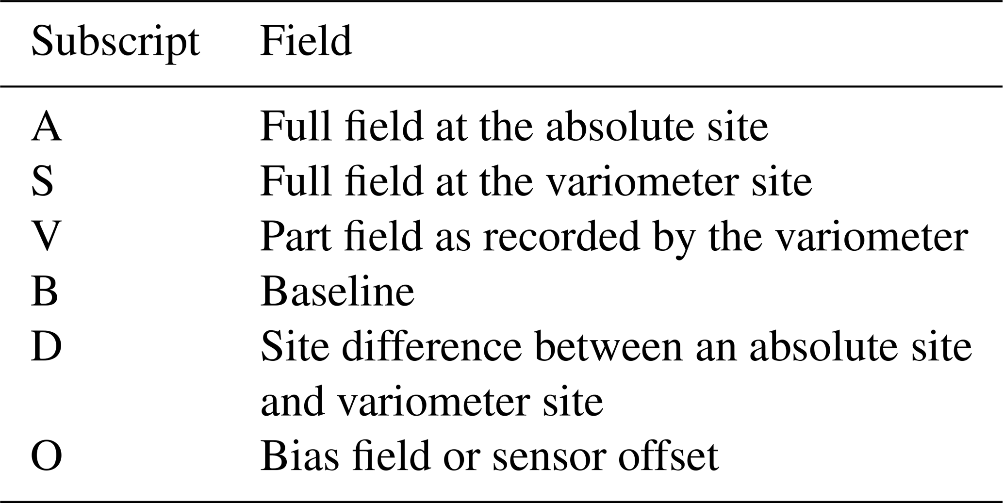
Table A1 defines the subscripts used to label the field measurements used in the baseline calculation. The measurements consist of full field, part field, baseline, and offset both at the absolute and variometer pillars.
The vertical sensor (Z), which is aligned vertically downward, measures the variation of the magnetic field at the variometer site (ZS(t)). Upon installation (t0), a bias field is applied to this sensor with the same magnitude but opposite direction to that of the main field, and thus the initial value is close to zero. At any time of measurement, the field is thus defined as ZV(t). The P and Q sensors are located in the horizontal plane, and the P sensor makes an angle D0 with true north (X) as shown in Fig. 3. In the installation, there is no bias applied to the orthogonal Q sensor because this sensor is rotated to the position where its value is zero (i.e. indicating the Q sensor is oriented in the magnetic east direction). This procedure will align the P sensor to the instantaneous horizontal field (magnetic north) at the variometer site HS(t0), and the angle D0 will approximate the instantaneous value of declination DS(t0). In the initial installation, the bias field is applied to the P sensor, and thus the output of the sensor in any point measurement is PV(t).
The Z baseline value can be determined by subtracting the absolute Z value (ZA(t)) from the variation ZV(t). In this calculation, the Z baseline also can be determined as the sum of the sensor offset (ZO(t)) and the site difference ZS(t).
A2 Horizontal component baseline
The H baseline can be processed similarly to the Z baseline; however, because both sensors (P and Q) cannot be assumed aligned or orthogonal to the H vector after the initial installation (owing to the field changing with time), the processing is slightly different. HS(t) can be determined from P and Q sensor values using vector relationships, as given by Eq. (A2).
The equation then can be re-expressed in terms of variometer output,
As noted above, there is no offset applied to the Q sensor, so Eq. (A3) becomes
Equation (A4) then can be written in terms of the field at the absolute site by adding the site difference.
The site difference of the Q sensor can be approximated to zero assuming the observatory is placed at a magnetic clean site with low gradient. In addition, PO(t)+PD(t) can be combined in terms of the baseline (PB(t)):
Finally, the baseline can be defined as follows:
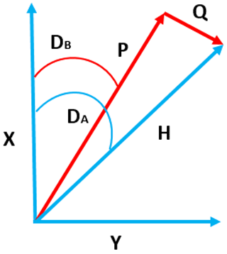
Figure A1Variation of declination angle at the variometer sensor. The difference between DA (absolute declination) and DB (baseline declination) is the declination variation in the variometer sensor.
A3 Declination component baseline
The declination baseline, DB(t), is an imaginary angle at the absolute site between absolute declination, DA(t), and variation (angle between QA(t) and HA(t)), as shown in Fig. A1. If the variometer is aligned such that the P sensor makes an angle (DB) to the true north, the angle of declination at the absolute site can be determined as
This equation can be written in terms of the variometer site:
Because the values of QO(t) and QD(t) are very small (and unknown), we can make the following approximation:
and the final baseline calculation can be written as follows:
The exact time of baseline calculation depends on the four circle readings of absolute measurement made using the theodolite, and thus the variometer data captured at the same time should also be averaged. If the baseline does not vary significantly, the baseline equation can be derived from the variometer data as in Eq. (A11).
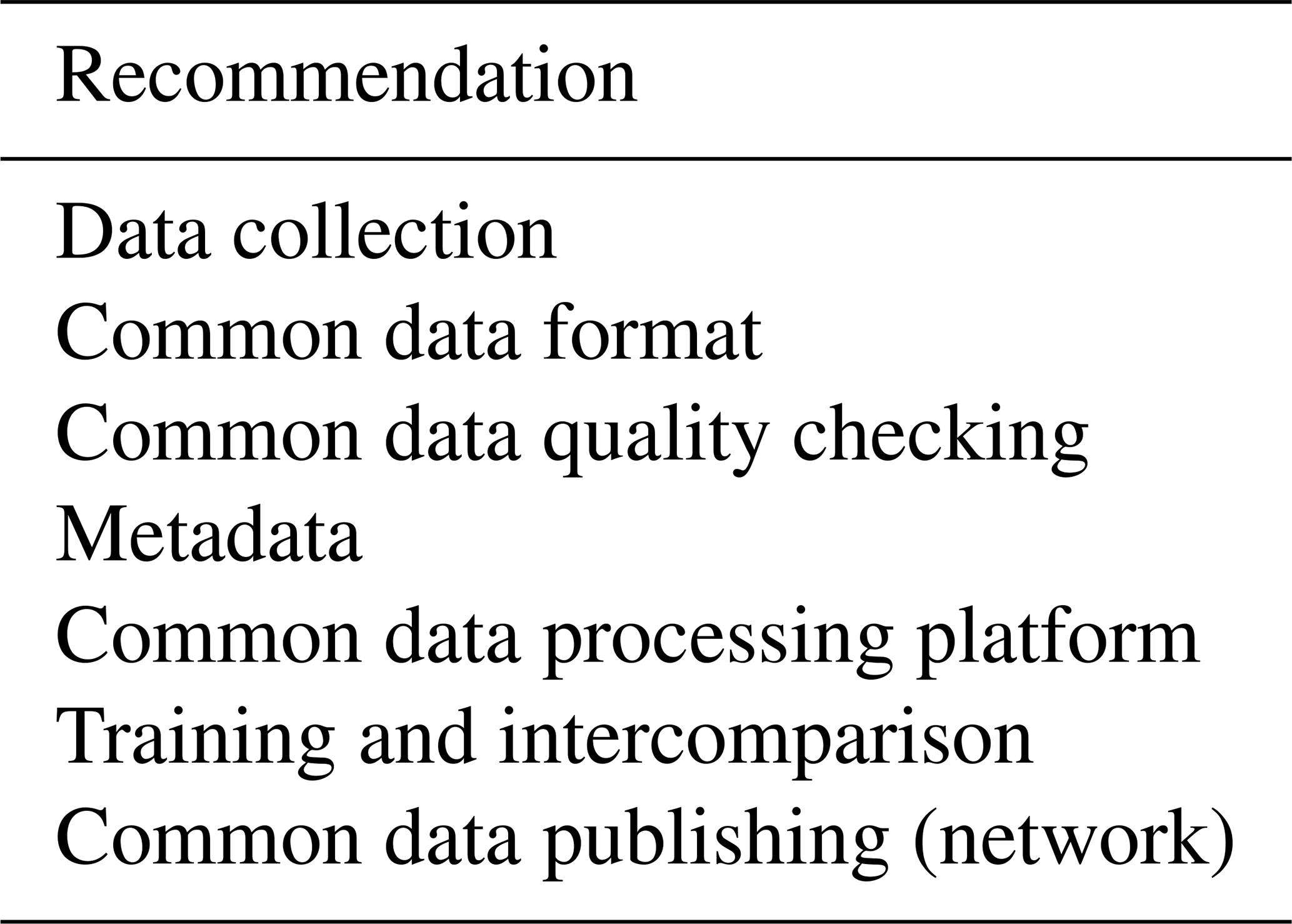
BMKG is the central institution for all geomagnetic observatories in Indonesia. If it can make good policy or provide standard operational procedures, it will have a strong impact on the quality of magnetic observatories in remote areas. Table B1 shows the summary recommendations for the central institution.
First, it is advisable to centralise the collection of data. Currently, this stage is achieved by the collection of raw data using a file transfer protocol (FTP) from the magnetic observatory to the central BMKG office. This data collection can be extended by including absolute observation data so that the central institution can make comparison results for the baselines.
Second, it is advisable to introduce standardisation of data reporting, including common data formats and sampling rates. This issue has been achieved by standardisation of all magnetic observatory raw data to 1 s data using the LEMI format. These raw data should be converted to the standard magnetic data format (e.g. IAGA-2002 format) after the raw data are processed and definitive data are produced.
Third, centralised quality control of data should be implemented. This can be done by day-to-day checking of the quality of raw data and weekly checking of absolute measurements. If the central institution finds an error in the raw data (noise, jumps, missing data, abnormal data), it should be confirmed with the observatory to determine what happened so that a quick solution can be found. In addition, BMKG also has to confer with the observatory if the absolute observation results are less accurate or a jump is identified in the baseline. It can request an alternative version or repeat of the absolute measurement. This aims to encourage observers to make absolute observations carefully. BMKG should also request additional measurements from the observatory, such as a site difference measurement, as this measurement is very important. A 3-month interval is appropriate and the results should be documented in the metadata. In addition, the temperature in the variometer building should be maintained constant as the sensor is temperature dependent.
Fourth, complete metadata should be stored at the central institution. The metadata consist of observatory instrument records, diaries of observatory changes, latitude, longitude, contact person, address, updated instrumentation, bulletin, and site plan. These metadata should be updated as soon as there are any changes at the observatory. These metadata are very important, especially if there is a problem in the data processing, as inaccurate metadata can produce errors in the data processing (e.g. sensor orientation).
Fifth, BMKG should provide a common data processing procedure. This procedure should state how to process raw data, absolute data, baseline calculations, and data transmission. These procedures can be accomplished by providing user-friendly software or a calculation template. BMKG should provide a guide and tools for standard data processing software (e.g. GDASview, MAGPY) or MATLAB scripts to be implemented at magnetic observatories. All the observatories should have a similar data processing procedure so that the output of the processing is standard. The implementation of the data processing can be given by on-site training or in a workshop.
Sixth, training of the observers should take place at least once a year. This training should attract observer representation from all Indonesian observatories. In the training or workshop, it is necessary to make an inter-comparison of instruments, simultaneous absolute observations, and practise data processing. The aims of this training are to produce standard approaches for all the observers and to build a network of colleagues that can advise and help each other.
Lastly, the observatory should publish their definitive data to the WDC so that the data can be used by the international community. In addition, each observatory should aspire to join INTERMAGNET or become certified so that its data quality will be assessed continuously by the organisation.
Table B1Summary of recommendations for Indonesian observatories.
The final definitive data have been published at WDC-G (http://www.wdc.bgs.ac.uk/dataportal, World Data Centre for Geomagnetism, 2021). The data can be accessed using IAGA's code for the following Indonesian Geomagnetic Observatories: TUN, PLR, TND, KPG.
RM initiated this paper, which is related to his MPhil studies. CWT guided the definitive data processing, including providing training in relevant software use, and CDB and KAW helped by providing useful discussions and in writing the manuscript.
The authors declare that they have no conflict of interest.
Publisher's note: Copernicus Publications remains neutral with regard to jurisdictional claims in published maps and institutional affiliations.
We thank all of the Indonesian geomagnetic observatory staff that helped with data requests and discussions (TUN: Yosi Setiawan; TND: Edward Mengko, Muhammad Zulkifli, Imam Muslih; KPG: Netrin Ndeo, Ricky Daniel, Aditya Nguru; PLR: Andi, Sofyan, Arafah; TNG: Dinda, Fani; JAY: Jambari; Central BMKG: Mahmud Yusuf, Aziz, Muhamad Syirojudin, Suaidi Ahadi). We are also grateful to the two anonymous reviewers for their valuable remarks that helped us to improve the paper. Relly Margiono also thanks John Riddick, who provided advice and useful discussions during this study. The research reported in this paper was begun during the MPhil programme of Relly Margiono at the University of Edinburgh.
This paper was edited by Luis Vazquez and reviewed by two anonymous referees.
Ahadi, S., Puspito, N. T., Ibrahim, G., Saroso, S., Yumoto, K., and Muzli: Anomalous ULF Emissions and Their Possible Association with the Strong Earthquakes in Sumatra, Indonesia, during 2007-2012, Journal of Mathematical and Fundamental Sciences, 47, 84–103, https://doi.org/10.5614/j.math.fund.sci.2015.47.1.7, 2015. a
Brown, W., Mound, J., and Livermore, P.: Jerks abound: An analysis of geomagnetic observatory data from 1957 to 2008, Phys. Earth Planet. In., 223, 62–76, https://doi.org/10.1016/j.pepi.2013.06.001, 2013. a, b
Chulliat, A., Macmillan, S., Alken, P., Beggan, C., Nair, M., Hamilton, B., Woods, A., Ridley, V., Maus, S., and Thomson, A.: The US/UK World Magnetic Model for 2015–2020, Tech. rep., BGS and NOAA, available at: http://nora.nerc.ac.uk/id/eprint/510709 (last access: 11 August 2021), 2015. a
Clarke, E., Baillie, O., J. Reay, S., and Turbitt, C. W.: A method for the near real-time production of quasi-definitive magnetic observatory data, Earth Planets Space, 65, 16, https://doi.org/10.5047/eps.2013.10.001, 2013. a
Cox, G. A., Brown, W. J., Billingham, L., and Holme, R.: MagPySV: A Python Package for Processing and Denoising Geomagnetic Observatory Data, Geochem. Geophy. Geosy., 19, 3347–3363, https://doi.org/10.1029/2018GC007714, 2018. a
Curto, J. and Marsal, S.: Quality control of Ebro magnetic observatory using momentary values, Earth Planets Space, 59, 1187–1196, https://doi.org/10.1186/BF03352066, 2007. a
Curto, J., Marshal, S., Torta, J., and Sanclement, E.: Removing Spikes from Magnetic Disturbances Caused by Trains at Ebro Observatory, in: Proceeding of the XIIIth IAGA Workshop on Geomagnetic Observatory Instruments, Data Acquisition, and Processing, available at: https://pubs.usgs.gov/of/2009/1226/ (last access: 11 August 2021), 2008. a
Finlay, C. C., Olsen, N., Kotsiaros, S., Gillet, N., and Tøffner-Clausen, L.: Recent geomagnetic secular variation from Swarm and ground observatories as estimated in the CHAOS-6 geomagnetic field model, Earth Planets Space, 68, 112, https://doi.org/10.1186/s40623-016-0486-1, 2016. a, b
Friis-Christensen, E., Lühr, H., and Hulot, G.: Swarm : A constellation to study the Earth's magnetic field, Earth Planets Space, 58, 351–358, https://doi.org/10.1186/BF03351933, 2006. a
Gillet, N., Barrois, O., and Finlay, C.: Stochastic forecasting of the geomagnetic field from the COV-OBS.x1 geomagnetic field model, and candidate models for IGRF-12, Earth Planets Space, 67, 1–14, https://doi.org/10.1186/s40623-015-0225-z, 2015. a
Gonsette, A., Rasson, J., and Humbled, F.: In situ vector calibration of magnetic observatories, Geosci. Instrum. Method. Data Syst., 6, 361–366, https://doi.org/10.5194/gi-6-361-2017, 2017. a
Jankowski, J. and Suckdorff, C.: Guide for Magnetic Measurement and Observatory Practice, IAGA, available at: http://www.iaga-aiga.org/publications/guides/ (last access: 11 August 2021), 1996. a, b, c
Khomutov, S. Y., Mandrikova, O. V., Budilova, E. A., Arora, K., and Manjula, L.: Noise in raw data from magnetic observatories, Geosci. Instrum. Method. Data Syst., 6, 329–343, https://doi.org/10.5194/gi-6-329-2017, 2017. a, b
Kloss, C. and Finlay, C. C.: Time-dependent low-latitude core flow and geomagnetic field acceleration pulses, Geophys. J. Int., 217, 140–168, https://doi.org/10.1093/gji/ggy545, 2019. a, b
Lviv: Fluxgate Magnetometer Lemi-018 User Manual, LVIV Centre of Institute of Space research, LVIV, Ukraine, 2008. a
McLean, S., Macmillan, S., Maus, S., Lesur, V., Thomson, A., and Dater, D.: US/UK World Magnetic Model for 2005-2010, Tech. rep., NOAA Technical Report NESDIS/NGDC-1, NOAA/BGS, Boulder/Edinburgh, 2004. a
Peltier, A. and Chulliat, A.: On the feasibility of promptly producing quasi-definitive magnetic observatory data, Earth Planets Space, 62, e5–e8, https://doi.org/10.5047/eps.2010.02.002, 2010. a
Pirjola, R.: Modelling the magnetic field caused by a DC-electrified railway with linearly changing leakage currents, Earth Planets Space, 63, 991–998, https://doi.org/10.5047/eps.2011.06.032, 2011. a
Poncelet, A., Gonsette, A., and Rasson, J.: Several years of experience with automatic DI-flux systems: theory, validation and results, Geosci. Instrum. Method. Data Syst., 6, 353–360, https://doi.org/10.5194/gi-6-353-2017, 2017. a
Rasson, J. L.: About Absolute Geomagnetic Measurements in the Observatory and in the Field, Institut Royal Météorologique, Institut Royal Météorologique De Belgique, Brussel, 2005. a, b
Rasson, J. L., Toh, H., and Yang, D.: The Global Geomagnetic Observatory Network, 1–25, Springer Netherlands, Dordrecht, https://doi.org/10.1007/978-90-481-9858-0_1, 2011. a, b
Reda, J., Fouassier, D., Isac, A., Linthe, H.-J., Matzka, J., and Turbitt, C. W.: Geomagnetic Observations and Models, Springer, 2011. a, b
Reigber, C., Lühr, H., and Schwintzer, P.: CHAMP mission status, Adv. Space Res., 30, 129–134, https://doi.org/10.1016/S0273-1177(02)00276-4, 2002. a
St-Louis, B.: INTERMAGNET Technical Reference Manual v4.6, Natural Resources Canada, Observatory Crescent, Ottawa, Ontario K1A 0 Y3, Canada, 2012. a
Sugiura, M. and Cain, J. C.: A model equatorial electrojet, J. Geophys. Res., 71, 1869–1877, https://doi.org/10.1029/JZ071i007p01869, 1966. a
Torta, J. M., Pavón-Carrasco, F. J., Marsal, S., and Finlay, C. C.: Evidence for a new geomagnetic jerk in 2014, Geophys. Res. Lett., 42, 7933–7940, https://doi.org/10.1002/2015GL065501, 2015. a
Turbitt, C.: Procedure for Determining Instantaneous GDAS Variometer Baselines from Absolute Observation, British Geological Survey, Edinburgh, 2003. a, b
World Data Centre for Geomagnetism: Geomagnetism Data Portal, available at: http://www.wdc.bgs.ac.uk/dataportal, last access: 10 August 2021. a
Zhang, S., Fu, C., He, Y., Yang, D., Li, Q., Zhao, X., and Wang, J.: Quality Control of Observation Data by the Geomagnetic Network of China, Data Sci. J., 15, p. 15, https://doi.org/10.5334/dsj-2016-015, 2016. a
- Abstract
- Introduction
- Data and methods
- Results
- Improving the entire processing chain
- Conclusions
- Appendix A: Baseline calculation
- Appendix B: Recommendations for Indonesian geomagnetic observatories
- Data availability
- Author contributions
- Competing interests
- Disclaimer
- Acknowledgements
- Review statement
- References