Passive seismic experiment “AniMaLS” in the Polish Sudetes (NE Variscides)

The paper presents information about the seismic experiment “AniMaLS” which aims to provide a new insight into the crust and upper mantle structure beneath the Polish Sudetes (NE margin of the Variscan orogen). The seismic network composed of 23 temporary broadband stations was operated continuously for about 2 years (October 2017 to October 2019). The dataset was complemented by records from eight permanent stations located in the study area and in the vicinity. The stations were deployed with an inter-station spacing of approximately 25–30 km. As a result, recordings of local, regional and teleseismic events were obtained. We describe the aims and motivation of the project, the station deployment procedure, as well as the characteristics of the temporary seismic network and of the permanent stations. Furthermore, this paper includes a description of important issues like data transmission setup, status monitoring systems, data quality control, near-surface geological structure beneath stations and related site effects, etc. Special attention was paid to verification of correct orientation of the sensors. The obtained dataset will be analysed using several seismic interpretation methods, including analysis of seismic anisotropy parameters, with the objective of extending knowledge about the lithospheric and sublithospheric structure and the tectonic evolution of the study area.

1 Introduction

The passive seismic experiment “AniMaLS” (Anisotropy of the Mantle beneath the Lower Silesia) aims at studying the structure of the crust and upper mantle of the Polish Sudetes and Sudetic Foreland, as well as the processes of their orogenic evolution, using seismological and petrological methods. Up to now, the upper mantle in this region was only sparsely sampled by seismic data (Wilde-Piórko et al., 1999, 2008). A temporary seismic array deployed in the Polish Sudetes in the period from October 2017 to October 2019 collected broadband seismological data, which are an important prerequisite to image the lithospheric and sublithospheric properties of the Sudetes and the Lower Silesia.

The Lower Silesian region comprises two major tectonic units: the Sudetes mountains and the Sudetic Foreland, forming the northeastern part of the Bohemian Massif (BM) and representing NE termination of the Variscan internides in central Europe (Figs. 1 and 2). The lithosphere of this area was consolidated during the Variscan orogeny (Late Devonian to Early Carboniferous) as the result of a multi-stage collision between the palaeocontinents of Laurussia and Gondwana and accretion of a group of smaller, Gondwana-derived Proterozoic to Palaeozoic microplates (Armorican Terrane Assemblage, ATA) at the Laurussian margin (Franke et al., 2017). Accreted Neoproterozoic to Cambrian metamorphic blocks and nappe complexes, as well as early Palaeozoic volcano-sedimentary rocks, were intruded by several Carboniferous granitoid plutons. In some parts, the region of the Sudetes was covered by sedimentary sequences of Late Carboniferous syn- and post-orogenic intramontane basins and Cretaceous to Cenozoic cover (Mazur et al., 2007).

Figure 1 Location map of the AniMaLS experiment. The red circles are the temporary broadband sites with 120 s sensors, the red squares are temporary sites with 30 s sensors, the dark red triangles are permanent stations (120 s sensors). Blue squares are short-period (1 s) temporary stations. LGCD is the Legnica–Głogów Copper District. The yellow star indicates epicentre of the local event discussed in Sect. 3. Elevation map based on GTOPO30 dataset (US Geological Survey, 1996).

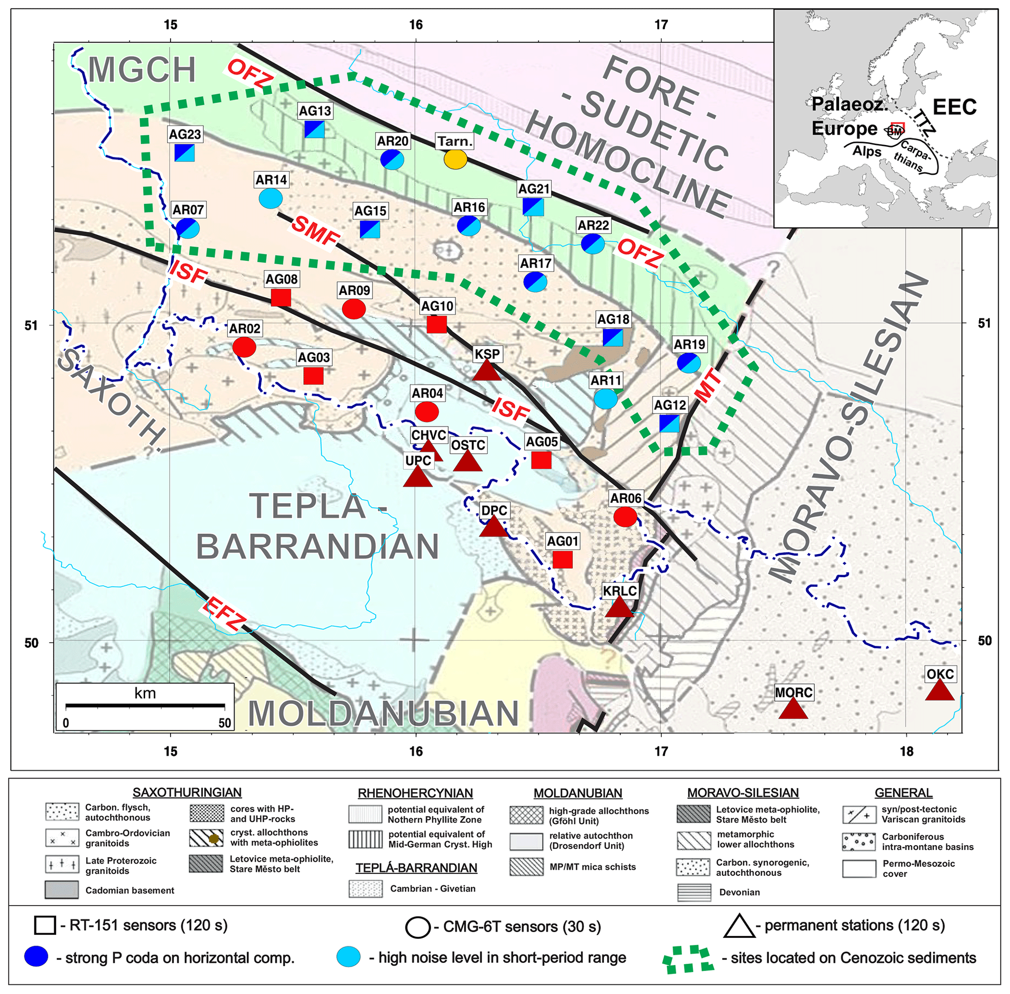
Figure 2 Locations of temporary (circles and squares) and permanent (triangles) stations used in the experiment on a background of a tectonic map (modified after Franke et al., 2017). BM – Bohemian Massif, EEC – East European Craton, EFZ – Elbe Fault Zone, ISF – Intra-Sudetic Fault, MGCH – Mid-German Crystalline High, MT – Moldanubian Thrust, OFZ – Odra Fault Zone, SMF – Sudetic Marginal Fault, TTZ – Teisseyre–Tornquist Zone. The dotted green line delimits area where observation sites are located on Cenozoic sediments. Other stations are mostly located on Palaeozoic or Proterozoic basement, and two stations are on Cretaceous rocks. Light blue marks – stations with high noise amplitude in the short-period range; dark blue marks – stations showing high amplitude, long coda of the P phase on horizontal components (see Sect. 3.1). Yellow circle – location of station in Tarnówek (Mendecki et al., 2016), discussed in Sect. 3.1.

At present, the lithosphere of the Sudetes is a mosaic of several units with distinct tectonic histories and with consolidation ages ranging from the upper Proterozoic to the Quaternary. The area is cut by three major right-lateral faults with WNW–ESE general orientation: Odra Fault Zone (OFZ), Sudetic Marginal Fault (SMF) and Intra-Sudetic Fault (ISF) (Aleksandrowski et al., 1997). The SMF divides the Sudetes block into the Sudetes mountains and Sudetic Foreland (Fig. 2). The mountain ridge originated from the Cenozoic rejuvenation and differential uplift of an old Variscan area due to collision-related intraplate stress at the Alpine foreland during the last episode of formation of the Alps and Carpathians. As a result of the uplift, the Sudetes mountains are the most exposed fragment of the NE Variscan basement in Europe (Mazur et al., 2007).

Due to complex structure of the region, several controversies and open questions concerning its evolution are still present – e.g. on the validity of the strike-slip tectonics model vs. oroclinal bending model as general mechanism responsible for the present-day lithospheric structure (Mazur et al., 2020), as well as more detailed issues, concerning, for instance, the roles of the regional fault and shear zones, the relationships between individual tectonic units and their ties to the structure and deformations of the underlying mantle. Therefore, the presented project attempts to provide new data on the structure, tectonic evolution and geodynamics of the NE Variscides with the use of seismic methods, based on recordings of local, regional and teleseismic events. The depth range of the experiment comprises the crust and the mantle lithosphere, the lithosphere–asthenosphere boundary (LAB) and the sublithospheric upper mantle.

Interpretation of the data with the P- and S-receiver function method will be attempted in order to trace the lithospheric and deeper (410 and 660 km) discontinuities. The project seeks to determine with more detail seismic anisotropy of the mantle with the use of the shear-wave-splitting method applied to SKS and SKKS phases. The analysis of the P-wave polarization may also contribute to anisotropy studies. Seismic anisotropy is closely related to mantle processes – its character reflects the degree and the direction of tectonic deformations of the lithosphere (or the orientation of the sublithospheric mantle flow). Potential spatial variations of anisotropy parameters can be a proxy for discrimination between lithospheric blocks with different petrological composition or subject to different tectonic evolution. Obtained seismic results will be complemented with information from ongoing petrological studies of anisotropy of the mantle xenoliths in the Cenozoic volcanics, abundant in the Sudetes (Puziewicz et al., 2015), in order to get more constraints on the nature of the mantle anisotropy. Acquired recordings of local events may also be useful for other fields of seismological research, e.g. for studies of the local seismicity, seismotectonics and seismic hazard assessment.

Previous seismic research on the Polish Sudetes involved mainly studies of the crust and sub-Moho mantle with wide-angle reflection/refraction method (e.g. Majdański et al., 2006; Růžek et al., 2007; Grad et al., 2008) or, recently, with ambient noise tomography (Kvapil et al., 2021). The upper mantle in this area was studied with various methods by the PASSEQ 2006–2008 experiment (e.g. Wilde-Piórko et al., 2008; Vecsey et al., 2014; Knapmeyer-Endrun et al., 2013). Numerous other seismic studies of the upper mantle, concentrating mainly on neighbouring parts of the Bohemian Massif, are also closely related to the objective of the presented experiment (e.g. Babuška, 2008; Kind et al., 2017; Geissler et al., 2012; Karousová et al., 2012; Plomerová et al., 2012).

The main purpose of this paper is to present the research objectives of the AniMaLS project, technical information concerning the data acquisition and obtained dataset. In Sect. 2.1, we describe the characteristics of the temporary seismic network and of the permanent stations in the study area. Also, in Sect. 2.2–2.5, we present details of the stations deployment procedure, including the site selection, sensor orientation, data transmission setup and status monitoring systems. We describe the technical aspects of field measurements, distribution, acquisition parameters of the stations and stages of data quality control. The near-surface geological setting of the sites is presented in Sect. 2.6. We describe data completeness and present data examples in Sect. 3. The noise characteristics, observed site effects and their relation to near-surface geology are discussed in Sect. 3.1. Finally, in Sect. 3.2, attention is paid to the data-based verification of the sensor orientation.

2 Station deployment

2.1 The network layout and equipment

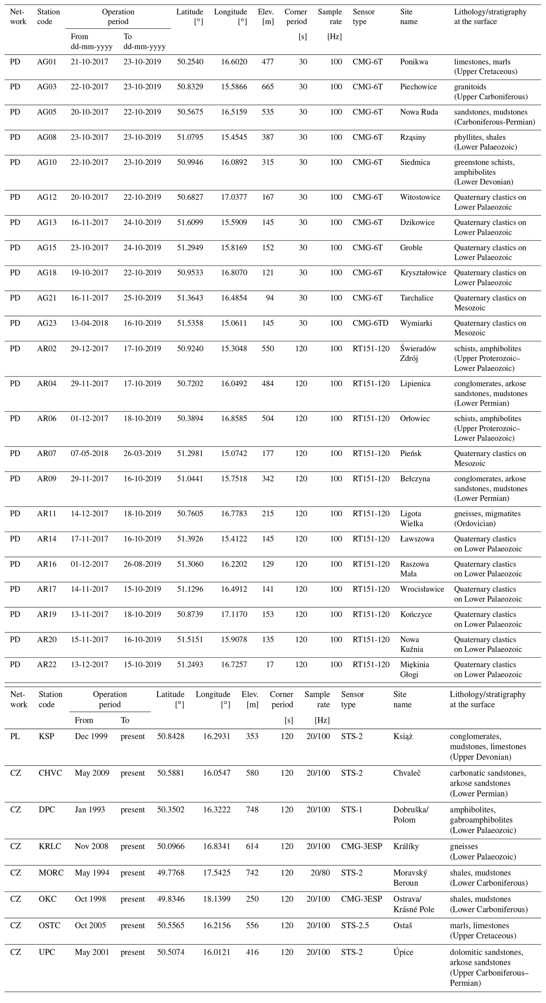
The AniMaLS seismic network had been deployed between October 2017 and January 2018 and was operated for a period of about 2 years, until October 2019. Two institutions contributed to the temporary seismic network – the Institute of Geophysics, Polish Academy of Sciences (IG PAS) provided 10 Güralp CMG-6T (30 s corner period) seismometers with Güralp DM24S3EAM data acquisition units and one CMG-6TD 30s seismometer and data acquisition unit. The Institute of Geophysics of the University of Warsaw (IG UW) supplied 12 Reftek-130B data acquisition systems with broadband seismometers Reftek 151–120 “Observer” with bandwidth of 0.0083–50 Hz (120–0.02 s). Additionally, for observations of local seismicity, IG PAS deployed six units with short-period (1 s corner period) Mark L-4C sensors. All stations had a 130 dB dynamic range and used 100 Hz sampling frequency. Timing was provided by GPS receivers. The average inter-station distance in the array was about 25–30 km.

As several permanent seismic stations were operated in the study area, it was possible to enlarge the dataset with recordings of stations: KSP (Polish Seismological Network) and CHVC, DPC, KRLC, MORC, OKC, OSTC and UPC (Czech Regional Seismic Network), all equipped with 120 s sensors. The short-period (1–5 s sensors) LUMINEOS network, designed by IG PAS for monitoring of the induced seismicity in Legnica-Głogów Copper District (LGCD) (Mirek and Rudziński, 2017), is also in the area we are investigating. The distribution of the AniMaLS stations and permanent seismic stations used in the experiment is shown in detail in Fig. 2. The coordinates of the stations, location names and technical details are summarized in Table 1.

2.2 Site selection and array design

Usually, the sites for permanent broadband seismic stations are carefully selected in areas with extremely low noise. The sensors are located in vaults designed to minimize noise resulting from thermal and atmospheric variations. Such a careful site preparation and installation is often not possible in the case of temporary seismic projects, where selection of the location, installation and formal issues (permissions, rental contracts) have to be done in a short time and with limited resources. Additionally, to form a more or less uniform network, the sites should be located at similar inter-station distances, which is another constraint for the site location. When deploying the array, we attempted to obtain a compromise between several factors: low seismic noise, site availability, continuous power supply and high signal level of the mobile telecommunications network (UMTS/LTE). An important issue was a high level of security, in order to avoid the damage or loss of the equipment. Meeting all these requirements was not straightforward, since in most of the locations the level of anthropogenic noise was elevated due to high population density and industrial activities. In these areas, fulfilling both constraints (station spacing and low noise) has been extremely hard. When possible, we placed the units at the unused basements of buildings, in the outbuildings or in rarely used public utility buildings. The sensors were placed on a hard surface – concrete or tiled floor, and in some cases a 5 cm thick granite slab was used for this.

At the sites, a thermal insulation of the sensor was ensured in the form of a styrofoam box covering the sensor. A few pictures from installation of a typical station are shown in Fig. 3. Each station was powered by a power grid system. The 12 V power supply was buffered with 40–60 Ah batteries in order to ensure continuous operation of the units in the case of the power outages. Near-real-time data transfer was done with the use of UMTS/LTE mobile network connection.

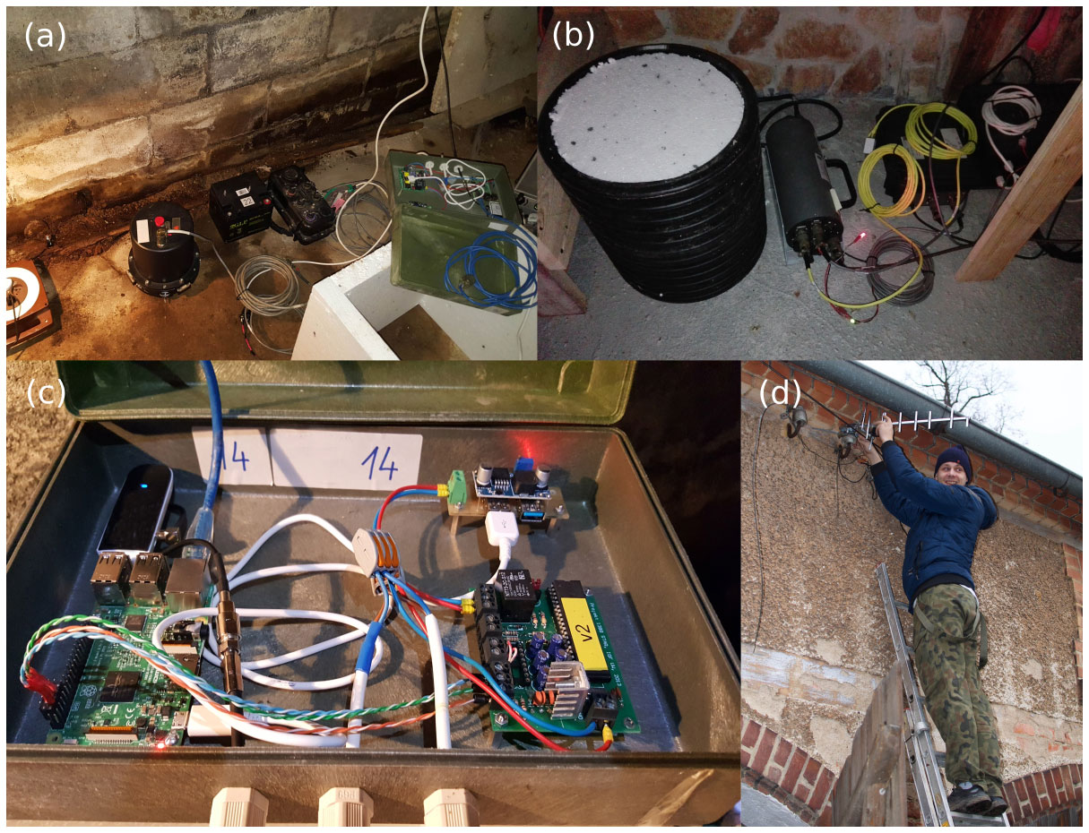
Figure 3 Deployment of seismic stations in the Sudetes: (a) Reftek unit during installation, (b) installed Güralp unit, (c) data-transmission module – Raspberry Pi microcomputer with UMTS modem and watchdog, (d) installing the UMTS antenna for data transmission.

2.3 Orientation of sensors

A precise orientation of seismic sensor axes with respect to geographical north direction is of great importance during installation of a three-component seismic station. Incorrect orientation of the seismometer can result in substantial errors when using three-component methods of interpretation, e.g. in the case of shear-wave-splitting analysis (Ekström and Busby, 2008; Vecsey et al., 2014; Wang et al., 2016). The simplest method of geographical north determination, using a magnetic compass, often results in uncertainty exceeding 5^∘ (Vecsey et al., 2017), which is not satisfactory for some interpretation methods. The modern approach, involving the use of an optical gyrocompass, allows for much higher precision but requires expensive equipment.

Taking these limitations into account, we have designed our own low-cost system for precise orientation of the seismometers deployed in the project. For the determination of the geographical north direction in the field, we used a global navigation satellite system (GNSS) unit with a real-time kinematic (RTK) positioning technology unit and ASG-EUPOS network (Ryczywolski et al., 2008) for receiving location corrections. Two ways for transferring the north direction to the seismometer location were considered. The first method was geodetic tacheometry. However, this method is not only time-consuming but also causes problems in less accessible locations such as basements. To solve this problem, we developed a simple device for azimuth transfer which makes the process more time efficient while retaining satisfactory precision.

The core of the device is a MEMS (micro-electro-mechanical system) triple-axis accelerometer and gyroscope unit MPU-6050, controlled by a single-board Raspberry Pi microcomputer. The data communication between device modules is based on I2C serial protocol over the general-purpose input/output (GPIO) ports. The code for processing the data from the gyroscope unit was written as a Python script. Raw data from the unit are converted into stable values of the rotation angle of the device. The problem of the gyroscope drift was solved by calibration of the immobile device prior to the measurement phase. During calibration the drift is evaluated, and, based on this, corrections for drift are continuously applied during the measurement.

Orienting the seismometer towards the geographic north with this method is done in two stages. First, GNSS RTK unit is used to obtain precise positions of two points of a baseline outside of the station site and to calculate the azimuth of the baseline as a reference. Next, the azimuth is transferred to the place where the seismometer will be installed. To this end, the gyroscope device is aligned parallel to the baseline using laser pointer, and a GNSS-measured reference azimuth value is used as input to the device. The device is then moved indoor to the station site where it is rotated to the north, according to displayed current azimuth, and the N–S line is marked on the floor at the location of the sensor. Finally, to check if the device readings were stable during the north measurement at the site, the device is moved back to the baseline and oriented along it, where, ideally, reference azimuth value should be again displayed. If the value differs substantially from the reference, it indicates excessive/variable drift or other errors, and the measurement is considered to be invalid. The procedure is repeated until two to three stable (negligible drift) and consistent measurements are obtained. Assuming availability of the GNSS RTK unit, this method is an affordable solution which allows for orientation of the sensor with the error determined in field tests to be at the level of ±2^∘. Additionally, a data-based verification of the orientations was done with use of polarization analysis. The results are discussed in Sect. 3.2.

Table 1 Location and technical parameters of the temporary and permanent stations used in the experiment, with lithology and stratigraphy information for observation sites.

2.4 Real-time data transmission and data storage

The seismic data were written in the internal storage of the data acquisition units (Güralps – 16 GB flash memory, Reftek 2 × 16 GB CF cards) and, simultaneously, they were transmitted in near-real time to dedicated acquisition servers at the IG PAS. Additionally, state of health (SOH) information including temperature, voltage and mass positions were transmitted. The data transmission was done using UMTS internet connection, with all devices running an IPsec VPN system to securely connect all the stations to the data acquisition server and to protect the system from unauthorized access. The Güralp units were connected to the network using Mikrotik routers with LTE modems. The data transfer to a dedicated CMG-NAM data hub was based on GDI protocol with a back-fill buffer, which allows for handling temporary loss of internet connection and retransmission of missing data packets after the connection is re-established. Connection loss and router/modem hang-up situations were handled by a data acquisition unit by an implemented software watchdog, which allowed for three levels of action: (1) soft reset of the modem, (2) power cycling of the modem and (3) power cycling of the unit and of the modem. For data transmission from Reftek units, a modified system designed at IG UW (Polkowski, 2016), based on Raspberry Pi Linux microcomputers with UMTS or LTE wireless modems was used. The Raspberry Pi units served both as routers and as devices scheduling the data transmission – collecting data from acquisition units and sending them to server (FTP, rsync and SSH protocols). The control scripts (PHP, bash) were designed to check for gaps in transferred data (due to, e.g. network connection loss, server or device hang-up) and to schedule data retransmission, if necessary. Hardware watchdog devices, designed at IG UW (Polkowski, 2016), were used to assure automatic restart of the transmitting unit on no connection or hang-up.

Both the Güralp and Reftek stations were remotely controlled and monitored using their proprietary software providing a WWW control interface. It allowed for checking the status of the individual units, mass positions, timing, voltages, temperature, as well as setting various recording parameters. For Reftek units, the control interface allowed for monitoring of mass positions and mass centring. Also, automatic mass centring could be triggered if mass voltages exceeded a threshold after a user-defined time.

The near-real-time data transfer has well-known advantages – inspection of the current data flow and access to current SOH information is useful for monitoring of the data quality and allows for fast detection of failures, such as power supply malfunctions or timing problems. Also, an increase of the noise level or the signal distortion due to an inadvertent moving or tilting of the sensor can be detected, and necessary station maintenance can be planned. This saves the number of the field trips needed for servicing the stations and helps to quickly re-establish proper acquisition of the seismic data.

The gaps in transmitted data resulting from the lack of UMTS connection were filled by periodic retrieving of the recorded data directly from the data acquisition system memory during stations maintenance in the field, if needed. The transmitted and patched data were stored in miniSEED format. After unification of information in headers, the daily miniSEED files were finally stored in the form of SeisComP data structure (SDS) – a hierarchical structure with file and directory naming convention which allows for easy access to the data, e.g. with the ObsPy package.

2.5 Station timing

The seismic studies require exact measurement of absolute time of the seismogram to be able to determine the arrival times of the analysed phases. An incorrect timing may lead to erroneous identification of the phases or incorrect travel-time determination. Currently, the seismic acquisition systems use GPS/GNSS receivers that allow for the synchronization of the internal clock with a high accuracy (±10 µs). However, in practice, technical malfunctions or loss of GNSS signal can introduce timing errors, and such problems should be recognized. If possible, incorrect timing should be corrected during initial data processing, or reported, to avoid using badly timed data for the interpretation. During the data acquisition for the project, an important problem with timing occurred for five Reftek acquisition units due to the “week number roll-over” (WNRO) issue in the GPS system in 2019, which affected the GPS receivers with older hardware that were not designed to cope with this issue. As a result, in July 2019, some of the stations started to report the date with wrong year (e.g. 2099) and incorrect day of year. However, the correct time of the day was preserved; therefore, it was easy to obtain the proper date by shifting the time by a fixed amount of full days. The corrected date/time was then written into miniSEED headers. Nevertheless, the wrong date caused malfunction of the online data transmission system, which expected a correct date in the transmitted file names and in the headers. The transmission system software had to be temporarily modified in order to avoid the problem. A permanent solution of the problem was later achieved by updating recorders' firmware with a patched, WNRO-aware version.

Other problem was detected at the AG23 station, equipped with CMG-6TD data logger: after a few weeks, the internal clock lost synchronization with GPS time, in spite of a properly working and locked GPS receiver. This resulted in a linear increase of the time difference, which reached ∼ 20 s after few months of recording. In this case, only an approximate time correction was possible. By comparing the timing of good-quality arrivals in seismograms from AG23 and neighbouring, correctly timed stations, it was possible to measure the time differences over the recording period and to apply appropriate corrections. Here, the accuracy of time determination after the correction was estimated to ∼ 1 s. This is a relatively large value, and it prevents such data from being used for modelling methods which require exact knowledge of the absolute time, as, e.g. seismic tomography. Nevertheless, such data can still be used in methods based on the relative time of the seismogram components, as receiver function method or shear-wave splitting. More precise determination of timing corrections for this station is planned with the use of a method based on the noise correlation between recordings from incorrectly timed station and neighbouring, correctly timed ones (Sens-Schönfelder, 2008).

2.6 Characteristics of observation sites and near-surface geology

The geology of the near-surface sequences varies considerably over the study area, ranging from Proterozoic crystalline rocks to unconsolidated Quaternary sequences. The geological structure of the basement at the observation site can heavily affect the character of the recorded seismograms; therefore, we summarize the differences in the near-surface lithology and discuss their possible influence on the seismic data. Table 1 presents locations, technical information (sensor type, operation time), lithology and stratigraphy at the site for temporary and permanent stations. Geological information is based on the Geological Map of Poland 1 : 500 000 (Państwowy Instytut Geologiczny – Państwowy Instytut Badawczy, 2021) and the Geological Map of Czech Republic 1 : 50 000 (Czech Geological Survey, 2021).

In the SW part of the study area (roughly corresponding to the Sudetes mountains), the observation sites are located directly on consolidated rocks of Palaeozoic or Proterozoic basement (except AG01 and OSTC, positioned on Cretaceous rocks). The stations in the NE (the less elevated region of Sudetic Foreland) are located on a layer of Cenozoic unconsolidated sediments, overlying the Palaeozoic basement. This area is marked in Fig. 3 with a dotted green line. The presence of the low-velocity Cenozoic deposits at these sites has a distinct influence on the seismic records, and a more detailed discussion of these effects is presented in Sect. 3.1.

3 Data

Figure 4 presents the epicentres of the earthquakes with magnitude above 5.5 which occurred during the registration period (October 2017–October 2019), according to the International Seismological Centre (2020) catalogue (1285 events). Figure 5 shows the data availability diagram for the stations of the network, produced using ObsPy package (Krischer et al., 2015). Several shorter gaps, mostly resulting from data transmission problems and some longer gaps (caused by hardware failures or power shortages due to heavy thunderstorms), are present. The overall completeness of the network-transmitted data, supplemented with untransmitted data after recovery in the field, is 97 %.

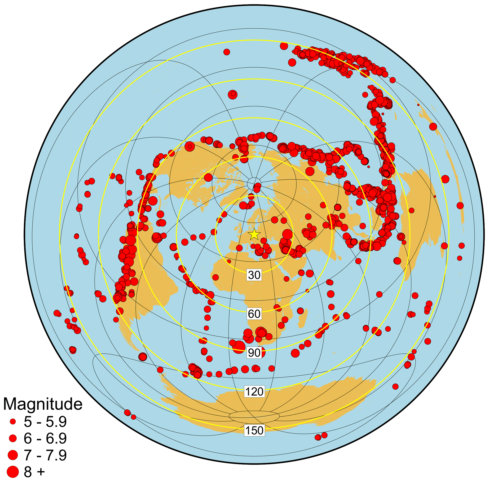
Figure 4 Distribution of the epicentres of M>5.5 earthquakes in the period from 18 October 2017 to 26 October 2019, according to the ISC catalogue (1285 events). The yellow asterisk represents the centre of the AniMaLS seismic array in the Sudetes. The yellow circles mark the distances (in degrees) from the array centre in 30^∘ steps.

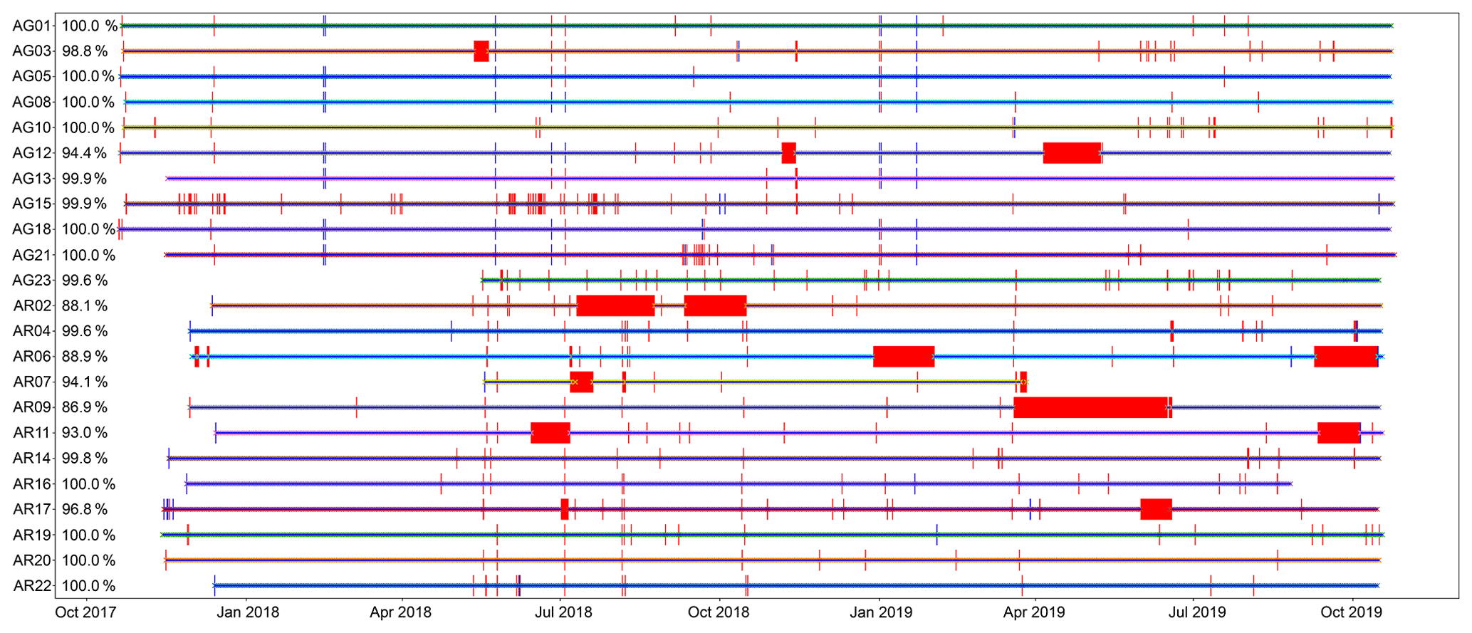
Figure 5 The diagram showing the data completeness for temporary stations. Red fragments – gaps in the data resulting from stations failures, memory card errors and power shortages.

Figure 6 presents an example of seismograms for an earthquake near Jan Mayen island. The seismograms show strong P-wave arrivals and lower-amplitude S arrivals, followed by high-amplitude surface (LR) waves, showing distinct dispersion. Figure 7 shows an example of a teleseismic earthquake from the Alaska area. Here, besides high-amplitude P and S waves, also free-surface reflections (PP, PPP, SS and SSS) can be clearly observed. Starting from ∼ 2050 s relative time, a long train of surface waves with substantial dispersion is visible. This figure clearly shows differences in frequency response of sensors for two groups of stations (it should be noted that records are scaled to maximum amplitude of each seismogram). For the AR (Reftek) and permanent stations, equipped with 120 s sensors, the strongest amplitude is seen for the earliest, long-period (∼ 50 s) pulses of surface wave at ∼ 2050–2150 s time. However, for AG stations, these long-period pulses are outside the 30 s corner frequency of the sensors and are strongly attenuated. With maximum trace amplitude scaling applied, this leads to substantial enhancement of amplitudes of remaining parts of the seismogram: the body-wave pulses and later surface wave trains (with periods < ∼ 30 s) for AG (Güralp) stations, relative to AR and permanent station records.

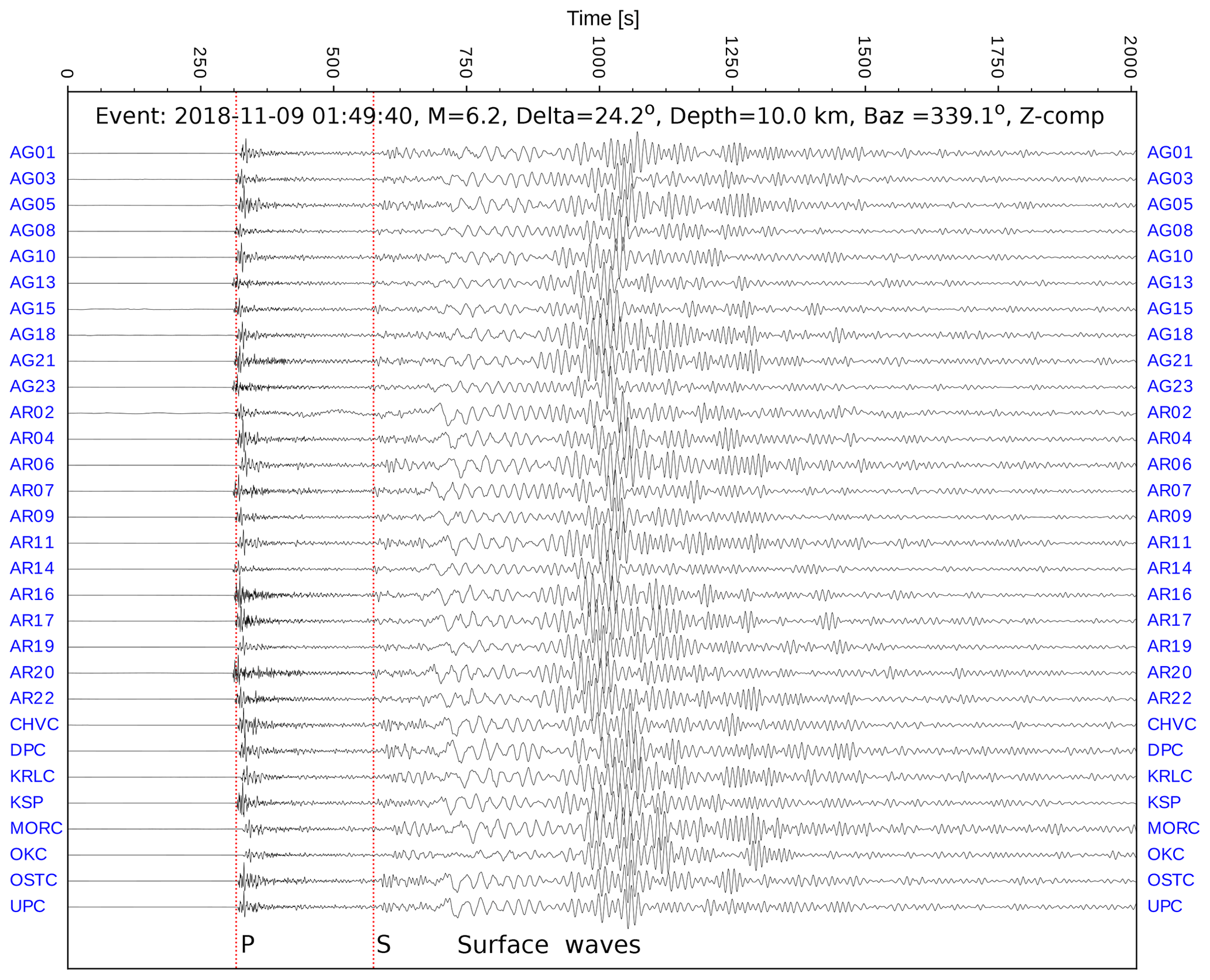
Figure 6 Example of vertical component of recorded waveforms for the M 6.2 teleseismic earthquake which occurred 9 November 2018 in Jan Mayen island region (lat: 71.6312, long: −11.2431, depth: 10.0 km after ISC). Red lines mark the theoretical onsets of P and S phases at the KSP station. All seismograms are low-pass filtered (<1 Hz).

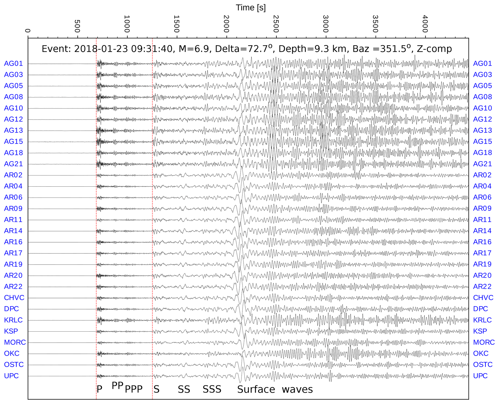
Figure 7 Example of vertical component of waveforms recorded for the M 6.9 teleseismic earthquake which occurred 23 January 2018 near Alaska (lat: 55.9315, long: −149.1877, depth: 9.3 km after ISC). Red lines mark the theoretical onsets of P and S phases at the KSP station. All seismograms are low-pass filtered (<1 Hz).

Figures 8 and 9 show local earthquakes from Legnica-Głogów Copper District and from Upper Silesia district, respectively. Both events are related to local mining activities. The figures show the Z component with 0.2–15 Hz bandpass filter. The epicentral distances are in the range of 0–240 km for the Legnica-Głogów event and 40–300 km for the Upper Silesia event. At these distances, we observe strong crustal phase (Pg) and mantle refraction (Pn phase) in the first arrivals. The Pn appears at offsets > ∼ 140 km. At larger times, strong S waves and surface waves are recorded.

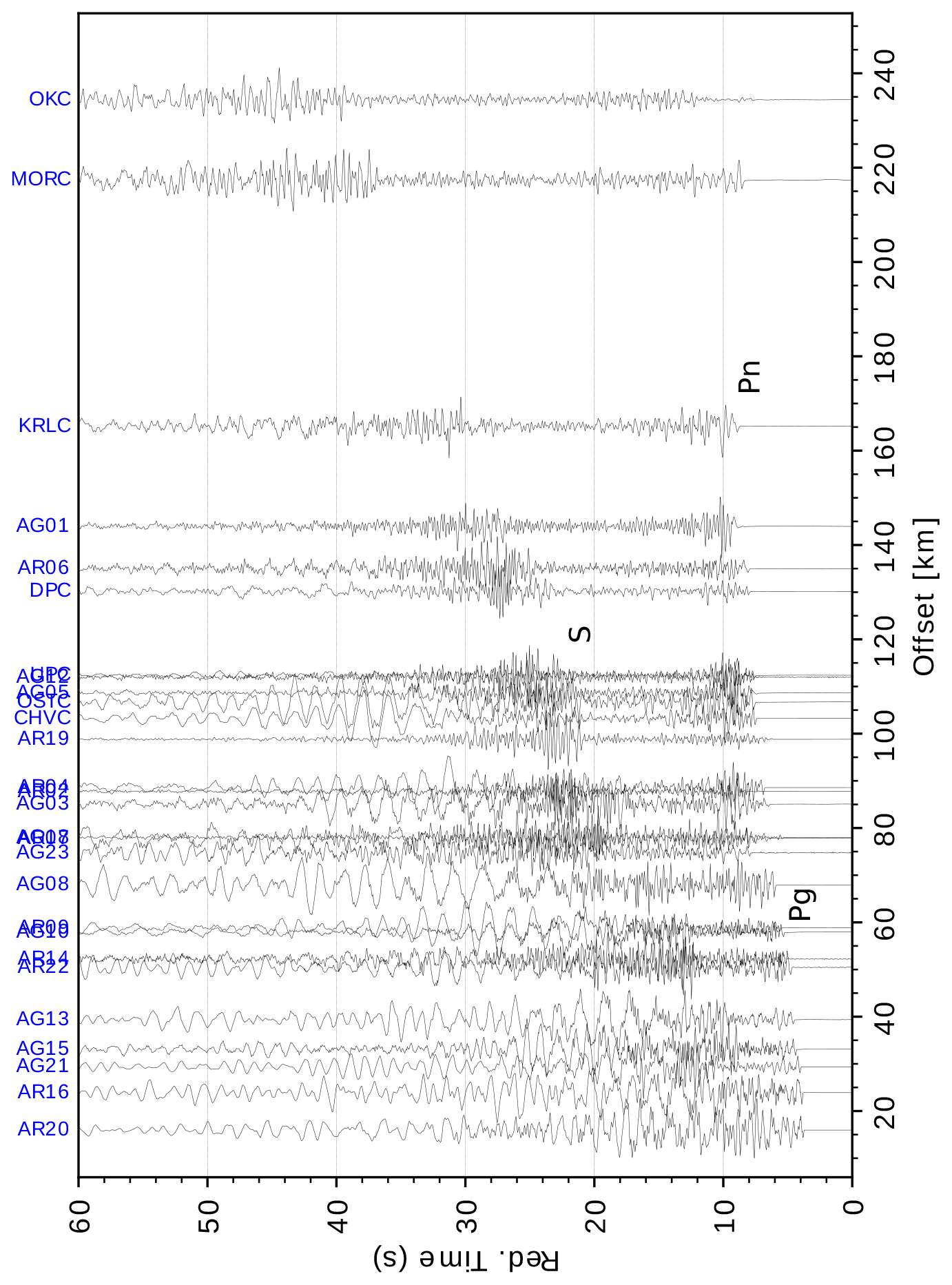
Figure 8 Example of waveforms recorded for the M4.4 local earthquake which occurred 3 July 2018, 19:38:47.75 UTC in Legnica-Głogów Copper District (lat: 51.5145, long: 16.1378, depth: 0.0 km after ISC). A band-pass filter of 0.2–15 Hz was used. Reduction velocity is 8 km/s. Location of the epicentre is shown in Fig. 2.

Figure 9 Example of waveforms recorded for the M3.9 local earthquake which occurred 22 January 2019, 22:35:30.08 UTC in Upper Silesia district (lat: 50.1095, long: 18.4559, depth: 5.5 km after ISC). Band-pass filter 0.2–15 Hz was used. Reduction velocity is 8 km/s.

An example of the time–frequency representation of the data is shown in Fig. 10. Here, a spectral seismogram obtained with the use of continuous wavelet transform (Daubechies, 1992) is presented for a teleseismic event (southern Alaska, epicentral distance 67^∘, back azimuth 353^∘) recorded by AR09 station. The Morlet wavelet was used. The onset of the P wave is visible at a ∼ 600 s relative time, in records of Z and N components, with maximum amplitude in the 2–4 s period range. At ∼ 1200 s travel time, the S waves with periods in the 12–15 s range are visible, with the largest amplitude on the E component. The body waves are much weaker than surface waves, which are visible at larger travel times. On the E component, corresponding approximately to transverse direction relative to ray back azimuth, the Love (LQ) waves with a period of 50–60 s can be seen at ∼ 1600 s time. The Rayleigh (LR) waves, best visible on N and Z component records at ∼ 1900 s, clearly show the dispersion, with period decreasing from 40 to 25 s.

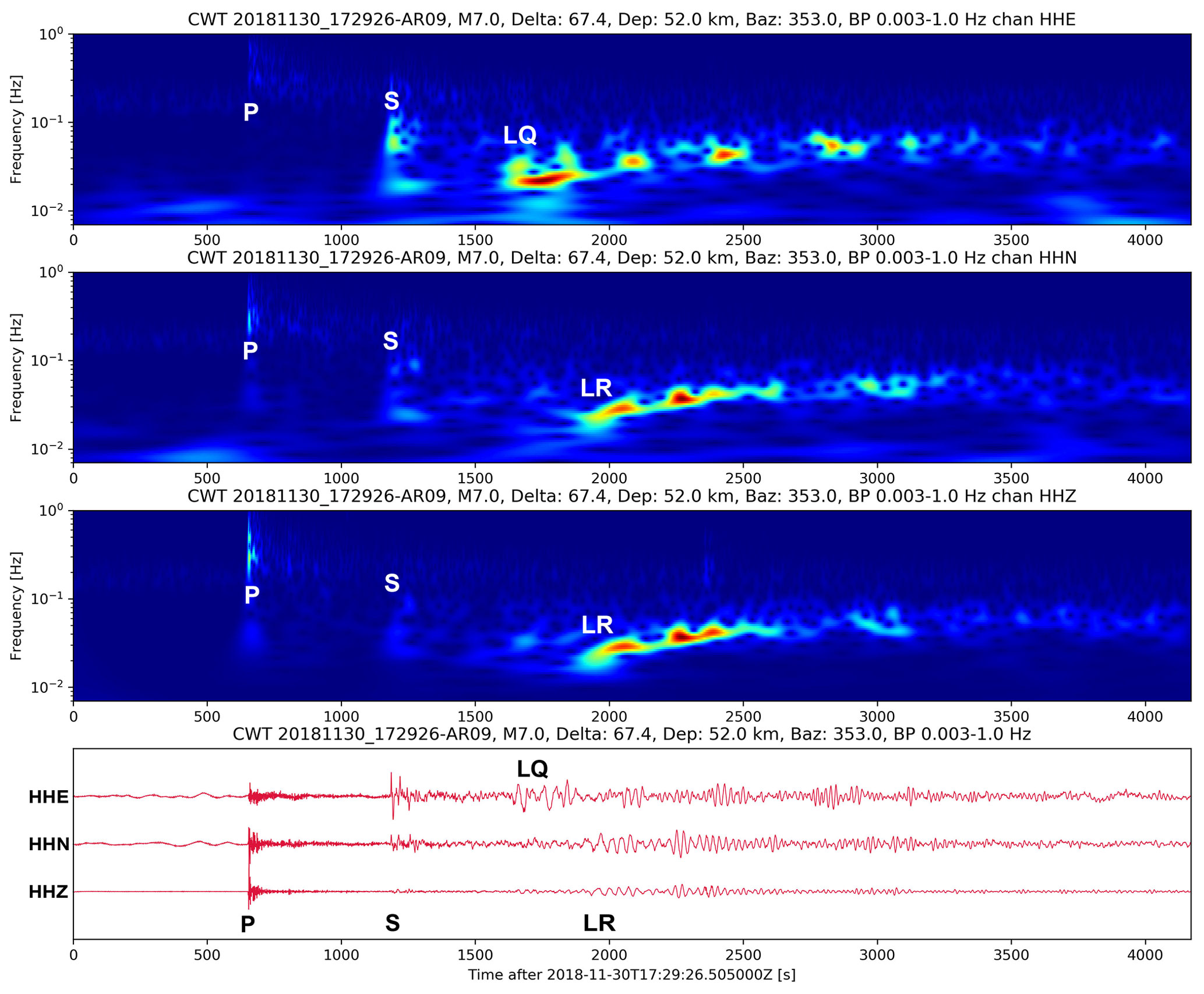
Figure 10 Spectral seismograms obtained with the use of continuous wavelet transform for station AR09, showing a teleseismic event from southern Alaska, 30 November 2018, 17:29:26 UTC. From top to bottom: E, N and Z components.

3.1 Seismic noise characteristics and site effect

To estimate the level of the ambient noise at various frequencies, we calculated the probabilistic power spectral density (PPSD) distributions (McNamara and Buland, 2004) for the data recorded at each station with the use of ObsPy package (Krischer et al., 2015). The PPSDs was calculated for continuous recordings from the period 1 December 2018–1 October 2019 (22 months).

The PPSD calculation was based on analysis of 1 h long windows of continuous seismic data (with 0.5 h overlap). The processing sequence consisted of demeaning, tapering, fast Fourier transform (FFT) computation and instrument response removal. The obtained frequency spectra for all windows were smoothed and summed to form a histogram representing the frequency distribution of noise amplitudes at various period ranges. The result shows which amplitudes are observed for a given period. The PPSD medians were also calculated.

Figure 11 shows a comparison of the PPSDs for three types of stations: AG10 (with 30 s CMG-6T sensor), AR06 (RT 151–120 s sensor) and permanent station UPC (STS-2 sensor). Diagrams for three components are presented. Figure 12 shows the PPSDs of Z component for 12 selected temporary and permanent stations used in this study (PPSDs for all stations are presented in Fig. S1 in the Supplement). Figure 13 shows a comparison of PPSD median curves for all sites used, including permanent and temporary stations. There is a systematic difference in the noise level between permanent and temporary sites. The difference is notable for long-period range (> 10 s) and is particularly large for the horizontal components. High amplitude of the noise for the long periods of the horizontal components is often experienced in the case of temporary stations, mainly due to an imperfect protection from environmental thermal/pressure changes or the sensor base tilt (Wilson et al., 2002). Another factor contributing to higher long-period amplitudes on the horizontal component with respect to vertical amplitudes, in particular for stations located on young/low velocity sediments, could be the ellipticity of the Rayleigh waves. In the presence of a low-velocity layer, the Rayleigh waves exhibit horizontally flattened particle motion, whereas at hard-rock sites on consolidated/crystalline basement, the particle motion is vertically elongated (Tanimoto et al., 2013). However, here, this factor seems to have a minor influence, considering relatively small (< 1 km) thickness of the low-velocity layer in this area, which should not affect the ellipticity of long-period (> 10 s) waves in question.

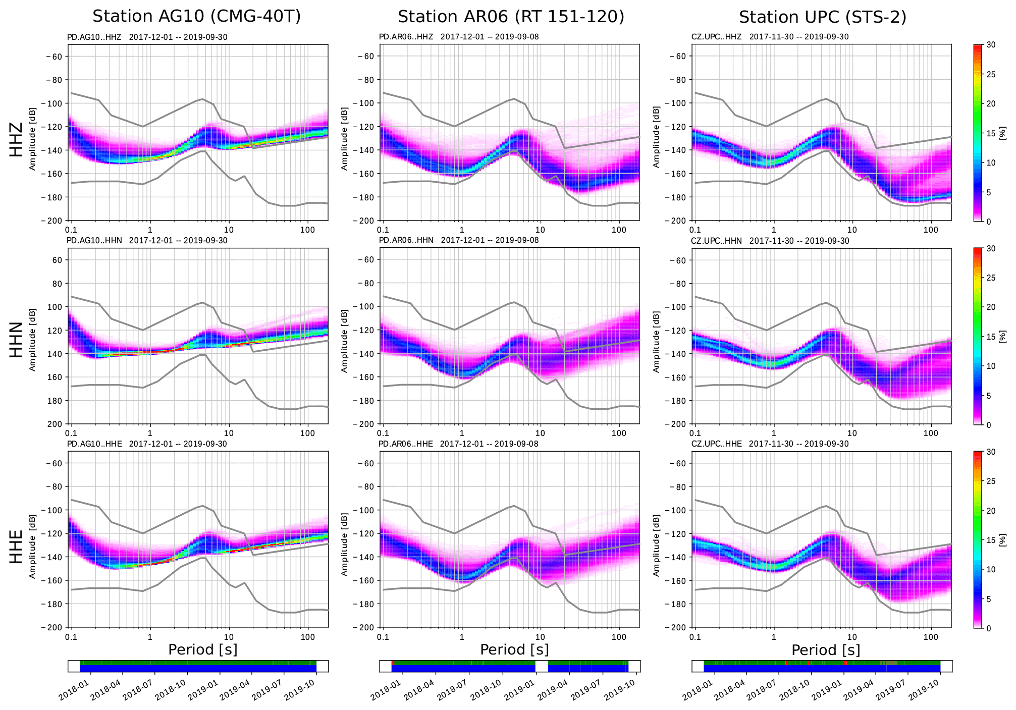
Figure 11 Probabilistic power spectral density (PPSD) for stations AG10 (CMG-6T), AR06 (RT 151–120) and permanent station UPC (STS-2). The Z, N and E components at the top, middle and bottom, respectively. The time span for calculation is 22 months (from January 2018 to October 2019). Black lines mark new high and low noise models (NHNM, NLNM; Peterson, 1993).

Figure 12 Probabilistic power spectral density (PPSD) on the Z component for 12 selected stations. (a) CMG-6T sensors, (b) RT 151–120 sensors, (c) permanent stations. Black lines mark new high and low noise models (NHNM, NLNM; Peterson, 1993).

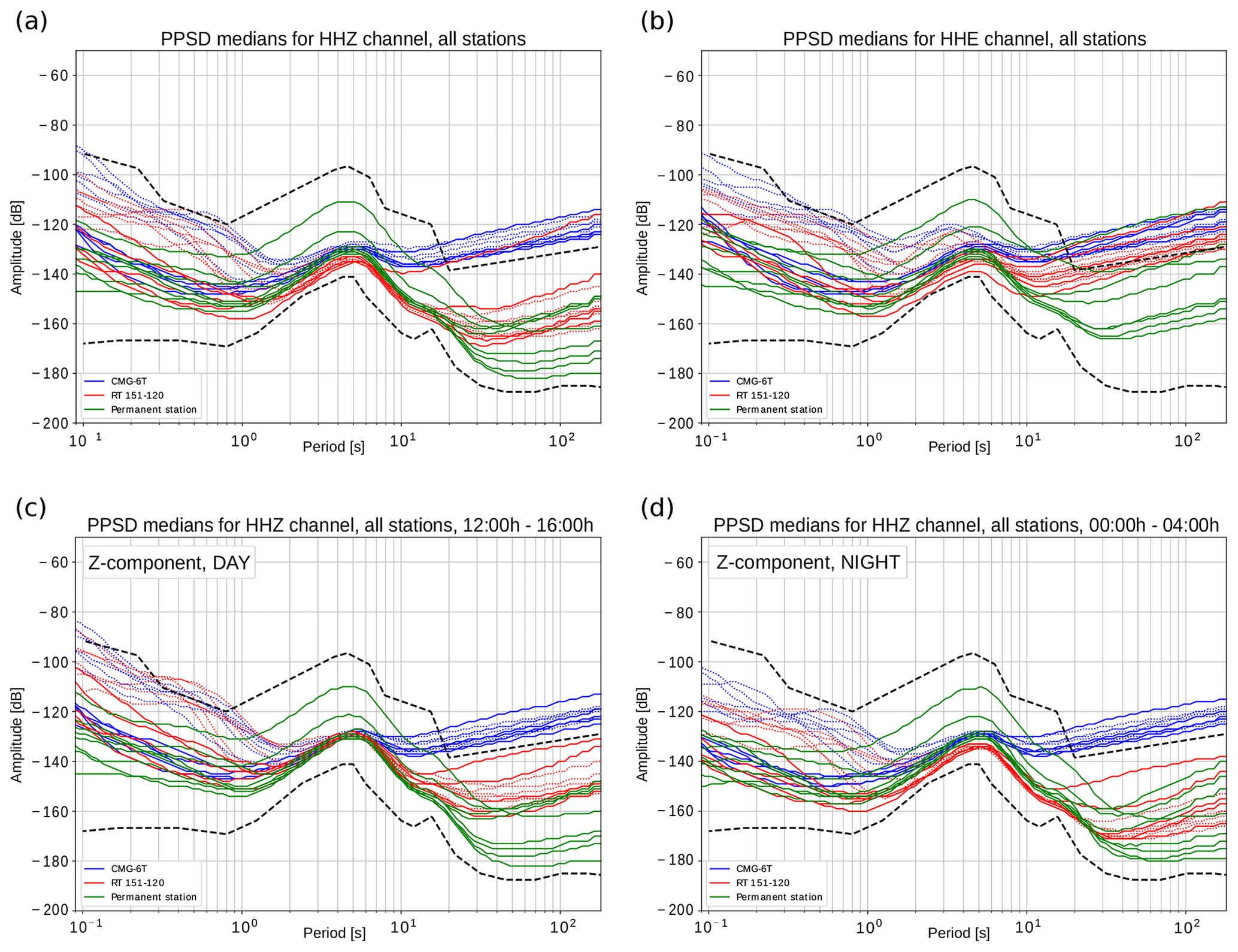
Figure 13 The PPSD median curves for all temporary and permanent stations. (a) Z component, (b) E component, (c) Z component, daytime hours only (12:00–16:00 LT), (d) Z component, nighttime hours only (00:00–04:00 LT). Dotted lines – stations located on Quaternary sediments, solid lines – stations located on Palaeozoic or older basement. Time span for calculation is 22 months (from January 2018 to October 2019). Black lines mark new high and low noise models (NHNM, NLNM; Peterson, 1993).

The highest amplitude of the long-period noise, often exceeding the new high noise model (NHNM) level, characterizes all sites with 30 s CMG-6T sensors. Similar behaviour of these sensors, independently of the actual noise at the site, was reported by Tilmann (2006). This is most likely due to high self-noise of this device type and, partially (for T_noise>30 s), to a lower corner period of the instrument (30 s vs. 120 s for other units). It is worth noting that the CMG-6T high long-period noise is at a very similar level to that for the ocean-bottom seismometer (OBS) version of the Güralp CMG-40T (30 s) sensor (Stähler et al., 2018), while the land version of CMG-40T shows substantially lower (by about 20 dB) self-noise in this period range (Custódio et al., 2014; Tasič and Runovc, 2012).

The short-period (SP) parts of the all PPSD medians (Fig. 13) show amplitude differences independent of the station type and can be subdivided into two groups. Stations located on Palaeozoic, or older, consolidated basement (solid lines in Fig. 13) show much lower noise in this part of the spectrum than the stations on the basement covered by unconsolidated, alluvial Cenozoic sequences (dotted lines). This area represents NE part of the network, marked with a dotted green line in Fig. 3. The stations with high amplitude of the short-period noise, marked with light blue colour, mostly fit into this region, which suggests a high correlation of this effect with the basement type. When attempting to interpret these differences in terms of the near-surface geology, care must be taken, because the high-noise sites installed on the Quaternary cover are, in the same time, located in the area with higher population density, denser network of roads, expressways and railroads, with typically higher anthropogenic noise. To check if the anthropogenic effects are responsible for these differences in short-period noise level, two variants of the PPSD medians were calculated for the same time span: only for daytime hours – from 12:00 to 16:00 LT, and only for nighttime hours – from 00:00 to 04:00 LT. Comparison of results (Fig. 13c, d) shows that the SP noise level during the daytime generally exceeds the nighttime noise by 5–15 dB for all stations, irrespective of their location. In the same time, differences in the short-period noise level between the sites located on old Palaeozoic rocks and the sites on the young Quaternary cover are of similar amplitude (∼ 25 dB) for day- and nighttime PPSDs, suggesting that they are indeed related to the basement type at the sites.

The presence of the low-velocity sediments in the area of Sudetic Foreland is also related to another effect, affecting the character of the P-phase onsets. The P-wave pulses on the horizontal components are followed by a prominent, high-amplitude coda/reverberations, extending over up to several hundreds of seconds (Fig. 14). The coda is characterized by a narrow frequency range, with a central frequency of 0.25–0.40 Hz (periods of 2.5–4 s), depending on the station location. The corresponding P pulses on the vertical component are much shorter and seem to be only weakly affected (or not affected) by the coda. In contrast, for the stations located on the consolidated basement, such reverberations are not observed on any component (Fig. 14a).

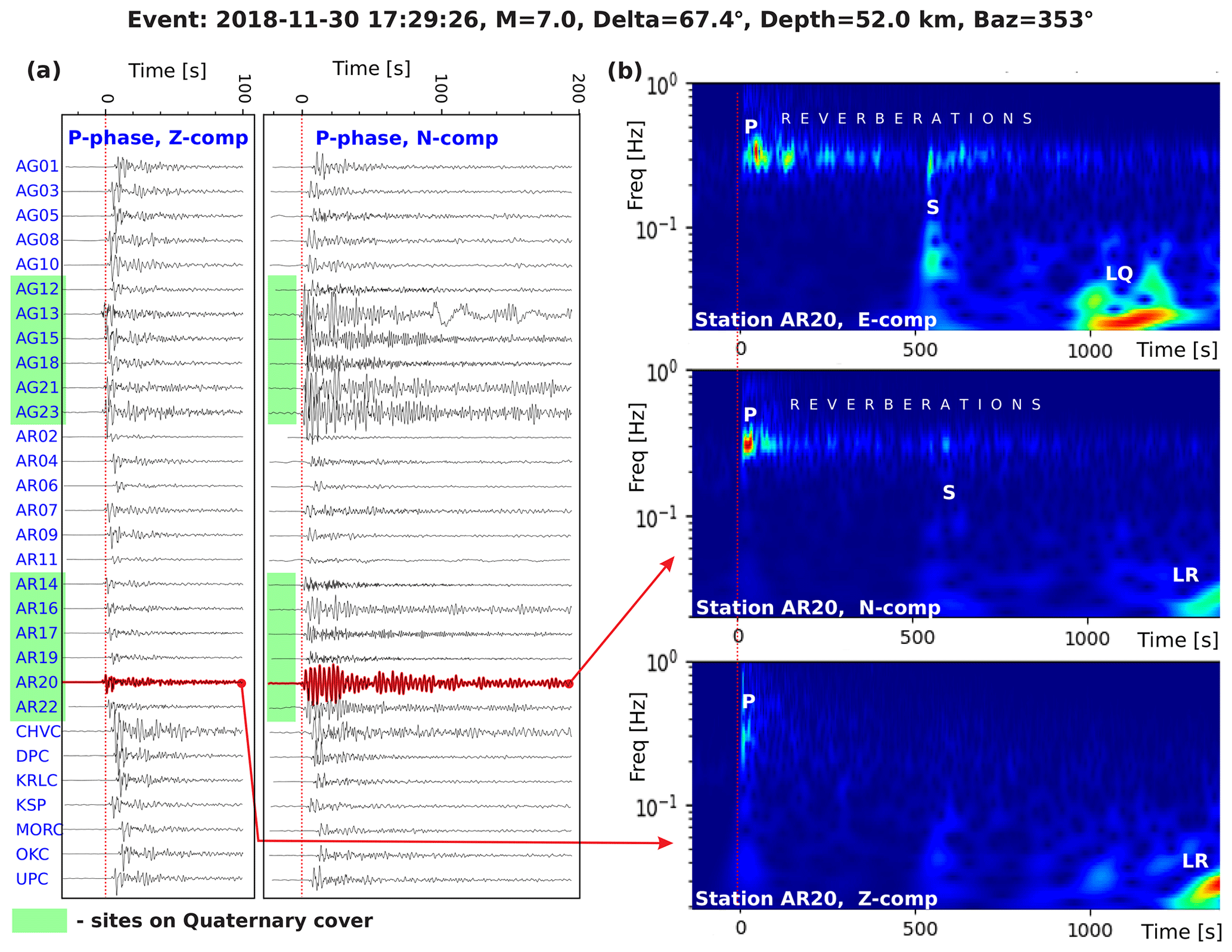
Figure 14 Seismic data example for event from 30 November 2018, 17:29:26 UTC, illustrating the differences in P-phase records between stations located on consolidated basement (short pulse, no reverberations) and sites located on young, unconsolidated cover (green rectangles, strong reverberations on the horizontal components). (a) Z and N component records for all the stations used. (b) Three-component spectral seismograms for station AG20. E and N components show high amplitude, >600 s long coda (reverberations) in a narrow frequency range, centred at 0.3 Hz. The coda is non-existent in the Z-component record. True amplitude scaling was applied. The timescale is relative to theoretical P-phase onset.

Such phenomenon is well known for a long time and described by several authors, e.g. by Zelt and Ellis (1999) or Yu et al. (2015), as it may heavily distort the results of the three-component interpretation methods. A layer of low-velocity sediments, with a strong impedance contrast relative to the consolidated or crystalline basement, produces multiple P-to-S conversions and reflections between the free surface and the base of the sediments. This results in high-amplitude reverberations in a narrow frequency range, mostly visible on the horizontal components. The frequency of the multiples is directly related to the seismic velocity and the thickness of the low-velocity layer. A systematic determination of the properties of the near-surface layer is out of scope of this paper. However, these observations can be compared with studies of the northeastern part of the study area (LGCD), where the properties of the low-velocity layer were studied by Mendecki et al. (2016). They used the horizontal-to-vertical spectral ratio (HVSR) method to analyse the resonance frequencies and amplification factors based on the data collected by a broadband station in Tarnówek (Fig. 3), located ∼ 15 km to the east of AR20 station. The HVSR peaks at 3.6–4.2 s were found, and V_s of ∼ 0.4 km/s was estimated for a ∼ 380 m thick Cenozoic layer at this location. In our study, the Fig. 14b shows a shorter (3.3 s) main period of the coda for AR20 station, which most likely corresponds to the thinning of the sedimentary layer or higher S-wave velocity.

The reverberations related to a low-velocity layer pose significant problems for the interpretation of the data, e.g. with the receiver function (RF) technique, as they overprint Ps conversion pulses on the radial component. One of the methods to overcome this problem was presented by Yu et al. (2015). As the reverberations exhibit a resonant frequency related to the two-way travel time of the wave in the sediment layer, the approach is based on designing a resonance removal filter in the frequency domain with filter parameters derived from the properties of the autocorrelation of the calculated RF. Our first tests showed that such a filter, applied to the data from Sudetic Foreland, is quite effective and significantly reduces the effect of reverberations.

3.2 Verification of sensors' misorientation

During the installation of stations in the field, to assure correct orientation, an azimuth measurement system with a GNSS RTK unit and a MEMS gyroscope was used, as described in Sect. 2.3. According to our estimates, such a system allows for determination of the north direction at the sensor location with ±2^∘ accuracy, if appropriate care is taken by the operator during all steps of the procedure. In order to additionally check for possible misorientation of the sensors after deployment, using the acquired data, a method based on the analysis of the P-wave polarization described by Fontaine et al. (2009) was applied. These estimates were verified with the use of a method proposed by Braunmiller et al. (2020), based on the P-wave polarization, and with the approach of Doran and Laske (2017) based on polarization of the Rayleigh waves. The two latter methods are implemented in the OrientPy package (Audet, 2020).

For a correctly oriented sensor and a homogeneous, isotropic medium, the polarization of the P-wave and of the Rayleigh wave particle motion is expected to be confined to the ray plane, and its horizontal component to be polarized parallel to the event back azimuth. The misorientation of the seismometer (deviation of the north seismometer axis from the geographical North by A degrees – equivalent to rotation of the coordinate frame of the measurement system) will obviously result in an apparent deviation of polarization of the P wave from the ray direction by an angle −A, independently of the event back azimuth. However, in a real medium, this deviation can be superimposed by the effects of the heterogeneity (dipping velocity discontinuities) or anisotropy of the medium under the station (Crampin et al., 1982; Schulte-Pelkum et al., 2001; Fontaine et al., 2009). These effects show a specific azimuthal dependence of resulting deviation angles (periodic with 180 or 360^∘ period); therefore, it is often possible to separate these factors, if data from a wide range of back azimuths are available. The total directional variability of the polarization deviation can be decomposed as (Schulte-Pelkum et al., 2001)

$$\begin{array}{}\text{(1)}& \begin{array}{rl}{D}_{\mathrm{pol}}\left(\mathit{\alpha }\right)& =A+B_{\sin }\left(\mathrm{2}\mathit{\alpha }\right)+C_{\cos }\left(\mathrm{2}\mathit{\alpha }\right)\\ & +D_{\sin }\left(\mathit{\alpha }\right)+E_{\cos }\left(\mathit{\alpha }\right),\end{array}\end{array}$$

where particular terms reflect the magnitude of various factors: A – the constant (azimuth-independent) component of polarization deviation, directly related to the incorrect sensor orientation; B and C – effect of anisotropy with horizontal symmetry axis; D and E – effect of anisotropy with inclined axis or effect of an inclined discontinuity; α – the event back azimuth.

For the analysis, from 165 events in the epicentral distance range of 5–100^∘, the recordings with high signal-to-noise ratio (SNR) on the vertical component of the P phase (SNR > 5) were selected for each station. Selected data were filtered (various sub-bands of 2–16 s period band were used) and 3-D particle motion at the P onset was analysed with the use of the orthogonal distance regression (ODR) method implemented in the ObsPy package, providing the azimuthal angle of the motion in the horizontal plane and incidence angle. Also, rectilinearity as defined by Fontaine et al. (2009) was calculated and was used to reject arrivals with poor rectilinearity of the particle motion, as contaminated by noise or other effects, and likely to produce distorted results. The error of the azimuthal angle was determined based on calculated eigenvalues of the particle motion (Fontaine et al., 2009). In order to improve stability of final results, individual D_pol values were sorted into back-azimuthal bins of 30^∘ width and averaged. Subsequently, these mean values were used for fitting the curve based on Eq. (1) and for calculation of A−E parameters. The constant parameter A corresponds to the sensor misorientation.

To verify the results, we also analysed the same dataset with a recently released software package OrientPy (Audet, 2020). The package implements two methods of determination of sensor orientation. The method described by Braunmiller et al. (2020) (BNG) determines the direction of P-wave polarization by minimizing the energy on the transverse component in a selected window around the P-wave onset (Wang et al., 2016). Subsequently, polarizations for all events are averaged. The averaged value represents the constant component of the azimuth-dependent deviations and is related to the misorientation angle for given station. It should be noted that the BNG method relies on relatively uniform back-azimuthal coverage of the analysed data – averaging of a non-uniformly sampled sinusoidal curve is likely to result in a biased estimate of the mean value. Obtaining the mean value A by fitting the function (Eq. 1) to the points as proposed by Fontaine et al. (2009) should produce a more reliable result if the azimuthal distribution of the data is highly inhomogeneous.

The Doran and Laske (2017) method (DL) is based on Rayleigh-wave polarization analysis. For each event, a search is done for an angle α (defined relatively to theoretical back azimuth) which maximizes the cross-correlation between the Hilbert transform of the vertical component and the radial component rotated by α. As in the BNG method, calculated individual deviations for all the analysed events are averaged to get a value of the misorientation of individual stations.

Figure 15 shows values of misorientations of all stations in the study area obtained with the use of three described methods; the permanent station GKP is outside the study area, but it is shown for comparison, as previous studies also reported its significant misorientation – Vecsey et al. (2014) reported 41^∘, Wilde-Piórko et al. (2017) reported 39 and 45^∘, and the result of this study is 34–37^∘. For many stations, the results derived from the three methods are more or less consistent but with some conspicuous exceptions. It can result from a small amount of recordings used for analysis because of low SNR for several stations.

Figure 15 Misorientation angles calculated for all stations using three described methods: red dots – Fontaine et al. (2009) method, green dots – BNG method, blue dots – DL method. Black circles with crosses – orientation angles of permanent stations from direct, high-accuracy measurements in field by gyrocompass (Luděk Vecsey, Institute of Geophysics of Czech Academy of Sciences, personal communication, 2020). Black squares with crosses (for GKP station) – orientation angles reported by other studies (Vecsey et al., 2014; Wilde-Piórko et al., 2017).

Table 2 Misorientation angles for all stations, obtained by different methods. Last column shows values from high-precision gyrocompass measurements or from other studies (if available).

^a Vecsey et al. (2014). ^b Wilde-Piórko et al. (2017).

For some permanent stations of the Czech Regional Seismic Network (CHVC, DPC, KRLC, OKC, OSTC and UPC), the orientation angles obtained from direct, high-accuracy gyrocompass measurements in field were available (Luděk Vecsey, Institute of Geophysics of Czech Academy of Sciences, personal communication, 2020). They are presented as a reference in Fig. 15. For almost all these stations (except CHVC) our results are in a good agreement (in a ± 2–3^∘ range) to the gyrocompass measurements.

It must be noted that the results of the indirect, polarization-based methods are not as precise as direct orientation measurements, e.g. with the optical gyrocompass. According to Rueda and Mezcua (2015), the Rayleigh wave polarization method achieves 1–5^∘ uncertainty in the case for long time spans of observations, e.g. at permanent stations, while for shorter time intervals the uncertainty can exceed 10^∘. Therefore, as pointed out by Vecsey et al. (2017), in the case of temporary arrays with limited period of data acquisition, the methods based on polarization analysis are able to detect only substantial ($>\sim$ 10^∘) misorientation of seismometers.

For most of the stations, the orientation values obtained from polarization analysis agree, within the error bounds, with the orientations measured directly at the sites with a GPS/gyroscope system, as can be seen in the Fig. 15 and in Table 2 (the estimated error bounds for both methods are $\sim \pm$ 3–7^∘ (largely) and ±2^∘, respectively). Therefore, we assume that the orientation of these stations determined by GPS/gyroscope can be considered as correct (0^∘ misorientation). However, for five other stations, the polarization analysis results differ significantly from the orientations measured at the sites – AR07, OSTC and GKP (absolute orientation values of ∼ 20–37^∘), CHVC and OKC (∼ 9^∘), suggesting that these sensors were incorrectly oriented during installation. The seismograms from these stations need to be rotated to a correct NE coordinate frame before use, and orientation codes in the headers of original (unrotated) data need to be set to Z, 1 and 2 instead of Z, N and E, according to the Standard for the Exchange of Earthquake Data (SEED) definition.

4 Conclusions and perspective

The AniMaLS project is an experimental seismic study of the physical properties and geological structure of the lithosphere and sublithospheric mantle beneath the Polish Sudetes (NE margin of the Variscan orogen), with a complex history of tectonic evolution. The acquisition of the seismic data involved deployment of 23 broadband stations for the period of about two years (October 2017–October 2019). The selection of sites and installation was done using a low-cost approach, with the stations deployed inside the unused basements, sheds or in rarely used public utility buildings. The stations were powered through the power grid, and the data were collected with the use of near-real-time data transmission over the UMTS network. During the measurement period, over 97 % of data were retrieved. Location of the sites in the inhabited areas increased the safety, the ease of installation and the reliability of the data transmission, however, at the cost of the noise level, which was higher compared to the permanent stations in the region. Overall, the installed network provided a reliable acquisition of the continuous, partly broadband seismic data in near-real time. The acquired records of local, regional and teleseismic events will be used as data for various seismic interpretation methods in order to determine velocity distribution, anisotropy and location of discontinuities in the upper mantle.

Obtained geophysical results will be integrated with geological research, as, e.g. studies of anisotropy of the mantle xenoliths from the Sudetes. A multidisciplinary synthesis involving the results of the seismic interpretation can serve as a basis for inferences about relative movements of the tectonic units forming the area, about the impact of orogenic and other deformational events on the present structure, and can help to reconstruct the history of geological evolution of the NE Variscan orogen and of the neighbouring areas.