Analysis and reduction of the geomagnetic gradient influence on aeromagnetic compensation in a towed bird

Aeromagnetic exploration is an important method of geophysical exploration. We study the compensation method of the towed bird system and establish the towed bird interference model. Due to the geomagnetic gradient changing greatly, the geomagnetic gradient is considered in the towed bird interference model. In this paper, we model the geomagnetic field gradient and analyze the influence of the towed bird system on the aeromagnetic compensation results. Finally, we apply the ridge regression method to solve the problem. We verify the feasibility of this compensation method through actual flight tests and further improve the data quality of the towed bird interference.

1 Introduction

Aeromagnetic exploration is generally used in geological research, mineral exploitation, and underground unexploded ordnance detection (Ekinci et al., 2020; Beamish and White, 2011; Doll et al., 2012). Since the magnetic field generated by the ferromagnetic material and metal-cutting geomagnetic wires on the aircraft platform will interfere with the magnetic detector, it will affect the quality of aeromagnetic survey data. Therefore, it is necessary to carry out aeromagnetic compensation (Chen et al., 2018).

In 1950, Tolles and Lawson (1950) summarized three sources related to aircraft maneuvers: the permanent field, the induced field, and the eddy current field. Leliak (1961) summarized the work of Tolles and Lawson and proposed a model of aeromagnetic compensation called the Tolles Lawson (T–L) model. As a linear solution, the T–L model faces the problem of multicollinearity (Leach, 1980; Bickel, 1979). In 1979, Bickel (1979) analyzed the multicollinearity of the T–L model and proposed a small signal solving method to reduce the linear relationship between features. In 1980, Leach used linear regression theory to study the T–L model and proposed a ridge regression algorithm to solve the multicollinearity problem in the T–L model (Leach, 1980). In recent years, the main methods to solve multicollinearity problems are the principal component analysis (Wu et al., 2018), the truncated singular value decomposition (TSVD) (Gu et al., 2013; Deng et al., 2013), the multi-model compensation method (Zhao et al., 2019), the wavelet analysis method (Deng et al., 2010; Dou et al., 2016a), and the improved recursive least-squares (Zhao et al., 2017). The above methods are all based on linear models. In 1993, Williams (1993) proposed a neural network nonlinear model to solve aeromagnetic interference, but this neural network model has an overfitting problem. On this basis, Ma et al. (2017) proposed a dual estimation compensation method of unscented Kalman filter and suppressed the problem of neural network overfitting by introducing measurement noise. Yu et al. (2021) proposed an aeromagnetic compensation model based on the generalized regression neural networks (GRNNs). The model combines linear regression and a neural network, which not only solves the insufficient fitting ability of linear regression but also weakens the influence of neural network overfitting. In practice, the measured value of the airborne magnetic sensor is the superposition of the geomagnetic field and interference field. The aeromagnetic interference value has been separated through a band-pass filter (Jia and Groom et al., 2004; Jia and Lo et al., 2004; Groom et al., 2004). However, due to the existence of a geomagnetic gradient, the filter cannot completely separate the geomagnetic field. In addition, the induced magnetic field component and the eddy current magnetic field component in the interference magnetic field are related to the geomagnetic field. Therefore, there is a strong coupling relationship between the geomagnetic field and magnetic interference (Dou et al., 2016b).

Figure 1 Towed bird system.

The measurement device and the electrified wire in the towed bird platform system will cause interference, so it is necessary to compensate for the interference of the towed bird platform. Because the towing bird system is affected by external factors, there are two modes of movement: swing and vibration. The swing amplitude is 10 m. The geomagnetic gradient is 0.5 nT m⁻¹, so the interference of the geomagnetic gradient on the towed bird is an important factor. In this paper, based on the towed bird interference model, the geomagnetic gradient component is introduced and solved by the ridge regression method. Through the actual flight data verification, this method can improve the data quality of pod interference.

Figure 2 Straight line and data.

2 Experiment and data introduction

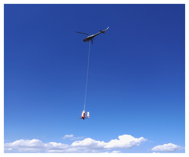
In the process of aeromagnetic exploration, most methods use fixed-wing platforms to compensate. When the magnetic sensor is located near the fuselage or inside the fuselage, the structure and changes of the interfering magnetic field generated by the aircraft in flight are complicated, which will also cause aeromagnetic interference (Xiu et al., 2018). To reduce the aeromagnetic interference, we used the helicopter towed bird method to conduct field test measurements in the Zhanhe area of Wudalianchi City, northern Heilongjiang Province. The towed bird is connected with the helicopter through a 30 m long rope in Fig. 1. Because the ferromagnetic material in the towed bird system will affect the measurement data of the magnetic sensor, it is necessary to compensate for the magnetic interference generated by the towed bird system. There are two kinds of motion modes in the motion process of the towed bird platform: one is the large amplitude swing mode influenced by the helicopter motion, the other is the amplitude vibration mode influenced by the wind speed. Under the joint action of the two motion modes, the measured data have interfered.

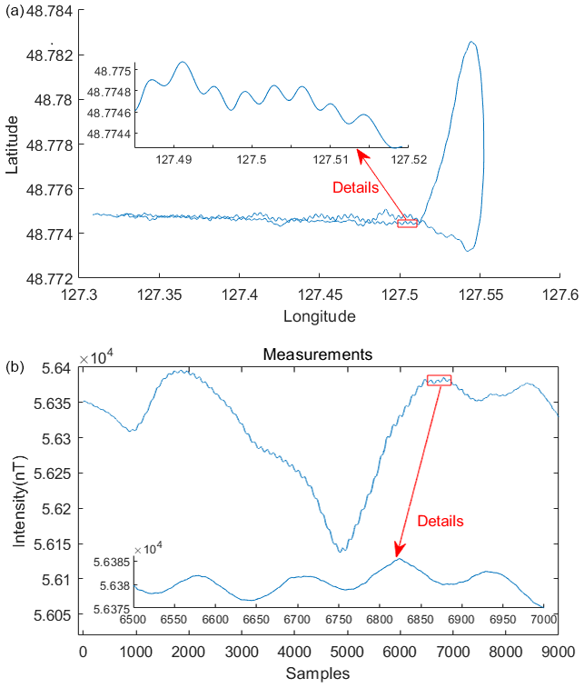
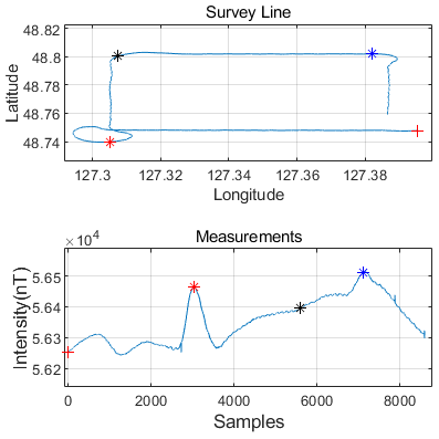
The experiment included three flights at an altitude of 1250 m. The first was a long straight flight. The purpose of the experiment was to observe the distribution of the geomagnetic field in the experimental area and the intensity of magnetic interference generated by the towed bird. Figure. 2a shows the flight path, where the survey line direction corresponds to the measured value in Fig. 2b. The swing range of the pod system platform is 10 m in Fig. 2a, and the measured value in Fig. 2b shows that the magnetic interference is about 5 nT. In Fig. 2b, the magnetic field difference between 5000–7000 sampling points is 250 nT. The distance is 500 m, so the geomagnetic gradient is 0.5 nT m⁻¹. In Fig. 3 the diamond data are used for the training of the aeromagnetic compensation model. In Fig. 4, square data are used as the verification of the training model.

Figure 3 Diamond line and data.

Figure 4 Square line and data.

3 Compensation method

3.1 Towed bird model

The interference generated by the towed bird system and the fixed-wing helicopter platform is caused by the magnetic sensor strap-down system platform.

Figure 5 The towed bird coordinate system.

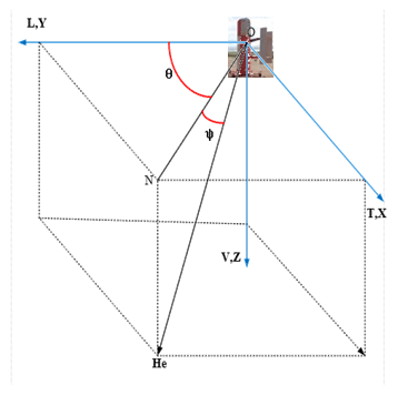
The towed bird coordinate system was established according to the fixed-wing coordinate system in Fig. 5 (Leliak, 1961). X, Y, and Z are the angles between the three coordinate axes of the towed bird and the geomagnetic field, called Euler angles, where θ and ψ are the geomagnetic declination and the geomagnetic inclination, respectively.

Euler angles X, Y, and Z can be measured by a three-axis magnetometer, and are redefined as follows:

$$\begin{array}{l}{\displaystyle }{u}_{\mathrm{1}}=\cos \left(X\right),\\ {\displaystyle }{u}_{\mathrm{2}}=\cos \left(Y\right),\\ \text{(1)}& {\displaystyle }{u}_{\mathrm{3}}=\cos \left(Z\right),\end{array}$$

where u₁, u₂, and u₃ represent the direction cosine of the Euler angle.

There are three types of magnetic field interference: permanent magnetic field, induced magnetic field, and eddy current magnetic field. Refer to the T–L model to establish the towing bird jamming platform model as follows:

$$\begin{array}{ll}{\displaystyle }{h}_{\mathrm{I}}=& {\displaystyle }{c}_{\mathrm{1}}{u}_{\mathrm{1}}+c_{\mathrm{2}}{u}_{\mathrm{2}}+c_{\mathrm{3}}{u}_{\mathrm{3}}+c_{\mathrm{4}}{u}_{\mathrm{1}}^{\mathrm{2}}+c{u}_{\mathrm{1}}{u}_{\mathrm{2}}+c_{\mathrm{6}}{u}_{\mathrm{1}}{u}_{\mathrm{3}}\\ {\displaystyle }& {\displaystyle }+c_{\mathrm{7}}{u}_{\mathrm{2}}{u}_{\mathrm{3}}+c_{\mathrm{8}}{u}_{\mathrm{3}}^{\mathrm{2}}+c_{\mathrm{9}}{u}_{\mathrm{1}}{u}_{\mathrm{1}}^{\prime }+c_{\mathrm{10}}{u}_{\mathrm{1}}{u}_{\mathrm{2}}^{\prime }+c_{\mathrm{11}}{u}_{\mathrm{1}}{u}_{\mathrm{3}}^{\prime }\\ \text{(2)}& {\displaystyle }& {\displaystyle }+c_{\mathrm{12}}{u}_{\mathrm{2}}{u}_{\mathrm{1}}^{\prime }+c_{\mathrm{13}}{u}_{\mathrm{2}}{u}_{\mathrm{3}}^{\prime }+c_{\mathrm{14}}{u}_{\mathrm{3}}{u}_{\mathrm{1}}^{\prime }+c_{\mathrm{15}}{u}_{\mathrm{3}}{u}_{\mathrm{2}}^{\prime }+c_{\mathrm{16}}{u}_{\mathrm{3}}{u}_{\mathrm{3}}^{\prime }.\end{array}$$

h_I is aeromagnetic interference. c_i, $i=\mathrm{1},\mathrm{2},\mathrm{3},\mathrm{\dots },\mathrm{16}$ is the aeromagnetic interference parameter. $u_{\mathrm{1}}^{\prime }$, $u_{\mathrm{2}}^{\prime }$, $u_{\mathrm{3}}^{\prime }$ is the derivative of Euler angle cosine to time.

This can be further expressed as follows:

$$\begin{array}{}\text{(3)}& h_{\mathrm{I}}=\mathit{u}\cdot \mathit{c},\end{array}$$

where c=[c₁ c₂ c₃…c₁₆]^T is the aeromagnetic interference parameter, and $\mathit{u}=\left[u_{\mathrm{1}}{u}_{\mathrm{2}}{u}_{\mathrm{3}}\mathrm{\dots }{u}_{\mathrm{3}}\right(u_{\mathrm{3}}{)}^{\prime }]$ is the aeromagnetic interference feature.

The linear superposition of geomagnetic field and aeromagnetic interference constitutes the measured value h:

$$\begin{array}{}\text{(4)}& h=H_{\mathrm{e}}+h_{\mathrm{I}}=H_{\mathrm{e}}+\mathit{u}\cdot \mathit{c}.\end{array}$$

3.2 Error analysis and improvement

Traditional aeromagnetic compensation usually uses a band-pass filter to obtain the aeromagnetic interference value. bpf(R) is expressed as linear band-pass filtering for each column of matrix R. Applying bpf to both ends of Eq. (4), we can get the following results:

$$\begin{array}{}\text{(5)}& \text{bpf}\left(h\right)=\text{bpf}(H_{\mathrm{e}}+\text{bpf}(\mathit{u}\cdot \mathit{c}\left)\right)=\text{bpf}\left(H_{\mathrm{e}}\right)+\text{bpf}\left(\mathit{u}\right)\cdot \mathit{c}.\end{array}$$

When bpf(H_e)=0, then

$$\begin{array}{}\text{(6)}& \text{bpf}\left(h\right)=\text{bpf}\left(\mathit{u}\right)\cdot \mathit{c}.\end{array}$$

The data processed by the band-pass filter are denoted as h_fu_f. Let $\text{bpf}\left(h\right)={\mathbf{h}}_{\mathrm{f}}\text{bpf}\left(\mathit{u}\right)={\mathbf{u}}_{\mathrm{f}}$. Then Eq. (6) can be expressed as follows:

$$\begin{array}{}\text{(7)}& {\mathbf{h}}_{\mathrm{f}}={\mathbf{u}}_{\mathrm{f}}\cdot \mathit{c}.\end{array}$$

Applying the least-squares method solves the following:

$$\begin{array}{}\text{(8)}& \mathit{c}={\left({\mathbf{u}}_{\mathrm{f}}^T{\mathbf{u}}_{\mathrm{f}}\right)}^{-\mathrm{1}}{\mathbf{u}}_{\mathrm{f}}^T{\mathbf{h}}_{\mathrm{f}}={\mathbf{u}}_{\mathrm{f}}^{+}{\mathbf{h}}_{\mathrm{f}},\end{array}$$

where ${\left({\mathbf{u}}_{\mathrm{f}}^T{\mathbf{u}}_{\mathrm{f}}\right)}^{-\mathrm{1}}{\mathbf{u}}_{\mathrm{f}}^T$ is the generalized inverse of the matrix u_f, denoted as ${\mathbf{u}}_{\mathrm{f}}^{+}$.

To analyze the influence of the system matrix u_f on the result, we perform singular value decomposition on the system matrix u_f:

$$\begin{array}{}\text{(9)}& {\mathbf{u}}_{\mathrm{f}}={\mathbf{USV}}^T={\sum }_{i=\mathrm{1}}^n{u}_{Ai}{\mathit{\sigma }}_{\mathrm{A}i}{v}_{\mathrm{A}i},\end{array}$$

where the matrix u_f is R×16 matrix. U and V are R×R and 16×16 orthogonal matrices respectively. S is R×16 diagonal matrix. σ_Ai is the ith singular value and has ${\mathit{\sigma }}_{\mathrm{A}\mathrm{1}}\ge {\mathit{\sigma }}_{\mathrm{A}\mathrm{2}}\mathrm{\dots }\ge {\mathit{\sigma }}_{\mathrm{A}n}$. u_Ai is the ith column vector of matrix U. v_Ai is the ith column vector of matrix V.

Then, the least-squares solution (Eq. 8) can be expressed as follows:

$$\begin{array}{}\text{(10)}& c={\sum }_{i=\mathrm{1}}^n{\displaystyle \frac{{\mathit{u}}_{\mathrm{A}i}^T{\mathbf{h}}_{\mathrm{f}}}{{\mathit{\sigma }}_{\mathrm{A}i}}}{v}_{\mathrm{A}i}.\end{array}$$

It can be obtained from the above formula that the system matrix u_f contains small singular values. The slight error in matrix h_f will be magnified. During the movement, the swing distance of the towed bird is 10 m. Since the geomagnetic gradient is 0.5 nT m⁻¹, it will introduce the geomagnetic gradient, resulting in the presence of the geomagnetic field component in the filtered aeromagnetic interference h_f, which will cause an error in the solution.

From the above analysis, it can be known that the existence of the geomagnetic gradient will affect the compensation result of the towed bird interference. According to the two-dimensional Taylor model of the geomagnetic field, the horizontal geomagnetic field is expressed as a function of latitude x and longitude y (Dawson and Newitt, 1977).

$$\begin{array}{}\text{(11)}& (H_{\mathrm{e}}{)}_{\text{hor}}={\sum }_{m=\mathrm{0}}^N{\sum }_{k=\mathrm{0}}^m{c}_{mk}(x-x_{\mathrm{0}}{)}^{m-k}(y-y_{\mathrm{0}}{)}^k,\end{array}$$

where (H_e)_hor is the horizontal geomagnetic field. x₀ and y₀ are the latitude and longitude of the initial position, c_mk is a constant, and N is the truncation order.

The filtered horizontal geomagnetic field obtained through band-pass filter processing is as follows:

$$\begin{array}{}\text{(12)}& \mathrm{\text{bpf}}\left({\left(H_{\mathrm{e}}\right)}_{\text{hor}}\right)=\text{bpf}\left({\sum }_{m=\mathrm{0}}^N{\sum }_{k=\mathrm{0}}^m{c}_{mk}{\left(x-x_{\mathrm{0}}\right)}^{n-k}{\left(y-y_{\mathrm{0}}\right)}^k\right).\end{array}$$

The Taylor model only considers the relationship between latitude and longitude and the geomagnetic field but does not consider the influence of altitude changes on the geomagnetic field. Since the helicopter's flying height is 1250 m, it is considered that the vertical geomagnetic field gradient is proportional to the helicopter's flying height. Assuming that the scale factor of the vertical gradient component of the geomagnetic field is v, the filtered vertical gradient component can be expressed as follows:

$$\begin{array}{}\text{(13)}& \text{bpf}\left({\left(H_{\mathrm{e}}\right)}_{\text{ver}}\right)=\text{bpf}\left(v\left(z-z_{\mathrm{0}}\right)\right)=v\text{bpf}\left(z\right),\end{array}$$

where bpf((H_e)_ver) is the filtered vertical geomagnetic field gradient value. z₀ is the height of the starting position of the towed bird, and z is the height of the towed bird during flight. Then the geomagnetic field passing through the band-pass filter can be further expressed as follows:

$$\begin{array}{}\text{(14)}& \begin{array}{rl}\text{bpf}\left(H_{\mathrm{e}}\right)& =\text{bpf}\left({\sum }_{m=\mathrm{0}}^N{\sum }_{k=\mathrm{0}}^m{c}_{mk}{\left(x-x_{\mathrm{0}}\right)}^{m-k}{\left(y-y_{\mathrm{0}}\right)}^k\right)\\ & +v\text{bpf}\left(z\right).\end{array}\end{array}$$

When the truncation order N is different, the expression of Eq. (14) will be different, which will affect the final compensation result.

Next, we use a band-pass filter to filter the truncation order $N=\mathrm{1},\mathrm{2},\mathrm{3},\mathrm{4}$:

$$\begin{array}{ll}{\displaystyle }N=\mathrm{1}& {\displaystyle }\text{bpf}\left(\right(H_{\mathrm{e}}{)}_{\text{hor1}})=c_{\mathrm{10}}\text{bpf}(x)+c_{\mathrm{11}}\text{bpf}(y),\\ {\displaystyle }N=\mathrm{2}& {\displaystyle }\text{bpf}\left(\right(H_{\mathrm{e}}{)}_{\text{hor2}})=c_{\mathrm{10}}\text{bpf}(x)+c_{\mathrm{11}}\text{bpf}(y)+c_{\mathrm{20}}\text{bpf}(x^{\mathrm{2}})\\ {\displaystyle }& {\displaystyle }+c_{\mathrm{22}}\text{bpf}\left(y^{\mathrm{2}}\right)+c_{\mathrm{21}}\text{bpf}\left(xy\right),\\ {\displaystyle }N=\mathrm{3}& {\displaystyle }\text{bpf}\left(\right(H_{\mathrm{e}}{)}_{\text{hor3}})=c_{\mathrm{10}}\text{bpf}(x)+c_{\mathrm{11}}\text{bpf}(y)+c_{\mathrm{20}}\text{bpf}(x^{\mathrm{2}})\\ {\displaystyle }& {\displaystyle }+c_{\mathrm{21}}\text{bpf}\left(xy\right)+c_{\mathrm{22}}\text{bpf}\left(y^{\mathrm{2}}\right)+c_{\mathrm{30}}\text{bpf}\left(x^{\mathrm{3}}\right)\\ {\displaystyle }& {\displaystyle }+c_{\mathrm{31}}\text{bpf}\left(x^{\mathrm{2}}y\right)+c_{\mathrm{32}}\text{bpf}\left(x{y}^{\mathrm{2}}\right)+c_{\mathrm{33}}\text{bpf}\left(y^{\mathrm{3}}\right),\\ {\displaystyle }N=\mathrm{4}& {\displaystyle }\text{bpf}\left(\right(H_{\mathrm{e}}{)}_{\text{hor4}})=c_{\mathrm{10}}\text{bpf}(x)+c_{\mathrm{11}}\text{bpf}(y)+c_{\mathrm{20}}\text{bpf}(x^{\mathrm{2}})\\ {\displaystyle }& {\displaystyle }+c_{\mathrm{21}}\text{bpf}\left(xy\right)+c_{\mathrm{22}}\text{bpf}\left(y^{\mathrm{2}}\right)+c_{\mathrm{30}}\text{bpf}\left(x^{\mathrm{3}}\right)\\ {\displaystyle }& {\displaystyle }+c_{\mathrm{31}}\text{bpf}\left(x^{\mathrm{2}}y\right)+c_{\mathrm{32}}\text{bpf}\left(x{y}^{\mathrm{2}}\right)+c_{\mathrm{33}}\text{bpf}\left(y^{\mathrm{3}}\right)\\ {\displaystyle }& {\displaystyle }+c_{\mathrm{40}}\text{bpf}\left(x^{\mathrm{4}}\right)+c_{\mathrm{41}}\text{bpf}\left(x^{\mathrm{3}}y\right)+c_{\mathrm{42}}\text{bpf}\left(x^{\mathrm{2}}{y}^{\mathrm{2}}\right)\\ {\displaystyle }& {\displaystyle }+c_{\mathrm{43}}\text{bpf}\left(x{y}^{\mathrm{3}}\right)+c_{\mathrm{44}}\text{bpf}\left(y^{\mathrm{4}}\right).\end{array}$$

By introducing Eq. (14) into Eq. (5), we can get the following results:

$$\begin{array}{ll}{\displaystyle }\text{bpf}\left(h\right)& {\displaystyle }=\text{bpf}(H_{\mathrm{e}}+\text{bpf}(\mathit{u}\cdot \mathit{c}\left)\right)=\text{bpf}\left(H_{\mathrm{e}}\right)+\text{bpf}\left(\mathit{u}\right)\cdot \mathit{c}\\ \text{(15)}& {\displaystyle }& {\displaystyle }=\text{bpf}\left(\right(H_{\mathrm{e}}{)}_{\text{hor}})+\mathit{v}\text{bpf}(z)+\text{bpf}(\mathit{u})\cdot \mathit{c}.\end{array}$$

bpf((H_e)_hor) can bring in different results according to different values of N in Eq. (14) and finally combine the towed bird model with the geomagnetic field model. The final expression is as follows:

$$\begin{array}{}\text{(16)}& \text{bpf}\left(h\right)=\text{bpf}\left({\mathit{u}}_{\mathit{\theta }}\right){\mathit{c}}_{\mathit{\theta }},\end{array}$$

where ${\mathit{u}}_{\mathit{\theta }}=[\mathit{u},z,x,y,x^{\mathrm{2}},\mathrm{\dots }]$ and ${\mathit{c}}_{\mathit{\theta }}=[\mathit{c},\mathit{v},c_{\mathrm{10}}{c}_{\mathrm{11}},c_{\mathrm{20}},\mathrm{\dots }]$. u_θ and c_θ have different expressions according to the value of N. For example, when N=1, ${\mathit{u}}_{\mathit{\theta }}=[\mathit{u},z,x,y]$ and ${\mathit{c}}_{\mathit{\theta }}=[\mathit{c},\mathit{v},c_{\mathrm{10}},c_{\mathrm{11}}]$.

Since the T–L model introduces the geomagnetic field component, the model will further have a multicollinearity problem. Therefore, the ridge regression method is introduced to solve this problem. The ridge regression solution formula is as follows:

$$\begin{array}{}\text{(17)}& \widehat{x_{\mathit{\theta }}}=\left({\left|\text{bpf}\left(h\right)-\text{bpf}\left({\mathit{u}}_{\mathit{\theta }}\right){\mathit{c}}_{\mathit{\theta }}\right|}^{\mathrm{2}}+\mathit{\lambda }{\left|{\mathit{c}}_{\mathit{\theta }}\right|}^{\mathrm{2}}\right),\end{array}$$

where $\widehat{{\mathit{c}}_{\mathit{\theta }}}$ is the parameter estimation value under the ridge regression, and λ is the regularization factor.

3.3 Evaluation standard of compensation quality

The traditional aeromagnetic compensation quality evaluation standard uses a standard deviation improvement ratio to evaluate the following:

$$\begin{array}{}\text{(18)}& \text{IR}={\displaystyle \frac{{\mathit{\sigma }}_{\text{before}}}{{\mathit{\sigma }}_{\text{after}}}}.\end{array}$$

σ_before and σ_after are the standard deviations of the data before and after compensation, respectively. Standard deviation data include not only aeromagnetic interference data but also geomagnetic gradient data. Assuming that the aeromagnetic interference and the geomagnetic field can be linearly superimposed, then

$$\begin{array}{}\text{(19)}& \text{IR}={\displaystyle \frac{{\mathit{\sigma }}_{\text{before}}^I+{\mathit{\sigma }}_{\text{before}}^E}{{\mathit{\sigma }}_{\text{after}}^I+{\mathit{\sigma }}_{\text{after}}^E}}.\end{array}$$

${\mathit{\sigma }}_{\text{before}}^I$ and ${\mathit{\sigma }}_{\text{after}}^I$ are the standard deviations of the aeromagnetic interference before and after compensation. ${\mathit{\sigma }}_{\text{before}}^E$ and ${\mathit{\sigma }}_{\text{after}}^E$ are the standard deviations of the geomagnetic field before and after compensation. The aeromagnetic interference caused by birds is small, but the geomagnetic gradient is large and changes a little before and after compensation.

$$\begin{array}{}\text{(20)}& {\mathit{\sigma }}_{\text{before}}^I\ll {\mathit{\sigma }}_{\text{before}}^E,{\mathit{\sigma }}_{\text{after}}^I\ll {\mathit{\sigma }}_{\text{after}}^E,{\mathit{\sigma }}_{\text{before}}^E\approx {\mathit{\sigma }}_{\text{after}}^E\end{array}$$

Therefore,

$$\begin{array}{}\text{(21)}& \text{IR}={\displaystyle \frac{{\mathit{\sigma }}_{\text{before}}^I+{\mathit{\sigma }}_{\text{before}}^E}{{\mathit{\sigma }}_{\text{after}}^I+{\mathit{\sigma }}_{\text{after}}^E}}\approx {\displaystyle \frac{{\mathit{\sigma }}_{\text{before}}^E}{{\mathit{\sigma }}_{\text{after}}^E}}=\mathrm{1}.\end{array}$$

Therefore, the data before and after compensation are filtered by a band-pass filter with a cut-off frequency of 0.03–0.1 Hz.

Then there are

$$\begin{array}{}\text{(22)}& \text{IR}\approx {\displaystyle \frac{{\mathit{\sigma }}_{\text{before}}^I}{{\mathit{\sigma }}_{\text{after}}^I}}.\end{array}$$

The paper takes IR as the evaluation index of the compensation result.

4 Results and analysis

According to the above analysis, when the truncation order of the two-dimensional Taylor model of the local magnetic field is $N=\mathrm{0},\mathrm{1},\mathrm{2},\mathrm{3},\mathrm{4}$, the ridge regression method is used to solve Eq. (17). The standard deviation IR of Eq. (22) is used to evaluate the results of aeromagnetic compensation.

Figure 6 Improved ratio (IR).

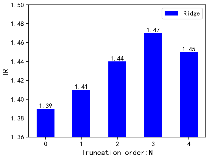
Figure 6 shows the standard deviation improvement ratio of applying the ridge regression method when the truncation order N is 0, 1, 2, 3, 4 respectively. The paper selects the truncation order of the two-dimensional Taylor of the geomagnetic field. When N=0, the compensation result is less than the standard deviation improvement rate when N is 1, 2, 3. When N is 4, it will be slightly lower than the standard deviation improvement ratio when N is 3. When the truncation order is greater than 3, the multicollinearity of the model will increase, leading to the introduction of errors in the solution process, so choosing a suitable truncation order is very important for model solving. When N is 3, the ridge regression method is used to solve the problem, and the final compensation result is the best. The standard deviation improvement is 6 % higher than that of the compensation effect without the geomagnetic gradient.

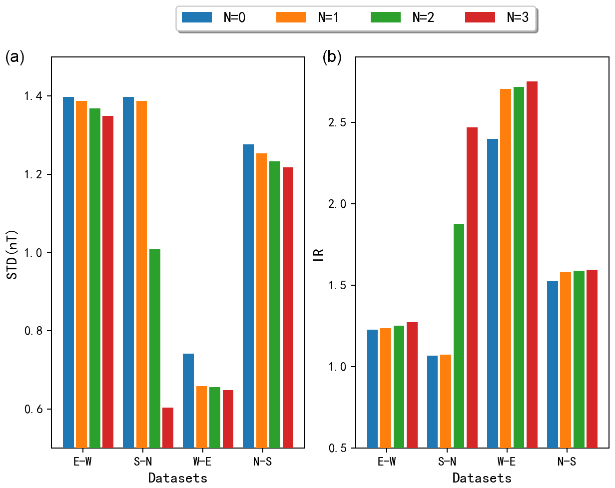
Figure 7 Comparison of compensation results of $N=\mathrm{0},\mathrm{1},\mathrm{2},\mathrm{3}$ in different directions: (a) standard deviation (SD) and (b) improvement ratio (IR).

Figure 8 Compensation result of $N=\mathrm{0},\mathrm{1},\mathrm{2},\mathrm{3}$.

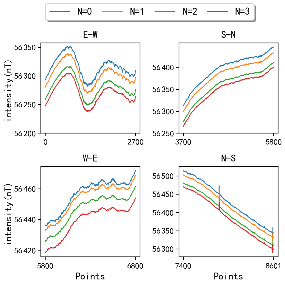
Figure 7 shows the comparison of the standard deviation and improvement ratio of the towed bird compensation in different directions. Figure 8 shows the comparison of the compensation result when $N=\mathrm{1},\mathrm{2},\mathrm{3},\mathrm{4}$. It can be seen from Figs. 7 and 8 that when the helicopter is flying in the south and west directions, the standard deviation is large, the towing bird swing is small, and the main interference is vibration mode. Therefore, when the geomagnetic gradient is introduced into the compensation, the result is only slightly better than the model when N=1. When the helicopter is heading north, because the towing bird platform is affected by swing and vibration, it is greatly affected by the geomagnetic gradient, resulting in large aeromagnetic interference. Introducing the geomagnetic gradient into the towed bird interference model will be improved, and IR will be improved to 2.47. When the helicopter is heading east, the interference is mainly caused by the swing mode of the towed bird. The standard deviation interference is small, and it is greatly affected by the geomagnetic gradient. So the IR is improved to 2.75.

5 Conclusion

The paper analyzes two movement modes of the towed bird system during the movement process. We considered the influence of geomagnetic gradient changes on the results of aeromagnetic interference compensation, but we also introduced the varying geomagnetic gradients into the interference model. Finally, we derive the model parameter estimation and correction. The paper solves the problem of the compensation result of the geomagnetic gradient change under the towing bird system but also expands the towing bird interference model. When the towed bird system is subject to large swings and vibrations in the heading, this method can improve the data quality of aeromagnetic interference; the experimental results show that the improvement ratio has increased by 6 %. Next, we will use this compensation method to improve the data quality of aeromagnetic surveys and use the helicopter towed bird system to detect underground magnetic targets.