the Creative Commons Attribution 4.0 License.
the Creative Commons Attribution 4.0 License.
 | 29 Apr 2022
Leveling airborne geophysical data using a unidirectional variational model
Qiong Zhang
Changchang Sun
Fei Yan
Chao Lv
Yunqing Liu
Airborne geophysical data leveling is an indispensable step in conventional data processing. Traditional data leveling methods mainly explore the leveling error properties in the time and frequency domain. A new technique is proposed to level airborne geophysical data in view of the image space properties of the leveling error, including directional distribution property and amplitude variety property. This work applied a unidirectional variational model to all the survey data based on the gradient difference between the leveling errors in flight line direction and the tie-line direction. Then, a spatially adaptive multi-scale model is introduced to iteratively decompose the leveling errors which effectively avoid the difficulty in parameter selection. Considering that anomaly data with large amplitude may hide the real data level, a leveling preprocessing method is given to construct a smooth field based on the gradient data. The leveling method can automatically extract the leveling errors of the entire survey area simultaneously without the participation of staff members or tie-line control. We have applied the method to the airborne electromagnetic and magnetic data and apparent-conductivity data collected by the Ontario Geological Survey to confirm its validity and robustness by comparing the results with the published data.
- Article
(9068 KB) - Full-text XML
- Companion paper
- BibTeX
- EndNote


Airborne geophysical surveys are widely used to produce geological mapping and mineral exploration that commonly adopt a continuous “S-type” flight mode at a particular elevation (Hood, 2007). In an airborne survey, the dynamic flight conditions cause unequal data levels, which are defined as leveling errors and shown as a stripe pattern along the flight direction. Leveling errors have a serious impact on airborne geophysical data analysis and interpretation.
A variety of factors contribute to the leveling errors, classified as the uncontrollable external environment and routine measuring mode. Airborne surveys in one measuring area usually have to last a particular number of months, and the environmental temperature has seasonal fluctuations and even regional fluctuations. Temperature variations can change the configuration of the survey aircraft used and affect its measuring hardware and the collected data (Huang and Fraser, 1999; Valleau, 2000; Siemon, 2009). Also worth noting is that the solar wind gives rise to geomagnetic diurnal variations in the earth's magnetic field (Yarger et al., 1978; Mauring et al., 2002). This is also regarded as leveling errors in airborne magnetic data.
The continuous S-type flight mode in measuring area brings opposite directions between adjacent lines, which leads to the survey aircraft being affected by different surrounding environments (Luyendyk, 1997; Gao et al., 2021). When the survey aircraft is blown by the wind in the opposite directions, the flight attitude angle may have minor difference, particularly for a helicopter-towed electromagnetic bird (Yin and Fraser, 2004; Huang, 2008). The temperature fluctuations also take place if the sun strikes the survey aircraft in different directions (Huang and Fraser, 1999). The fluctuations are uncontrollable and hard to compensate for, which contributes to leveling errors.
In addition, altitude variation is the source of the leveling errors in airborne electromagnetic (AEM) data. Although the drape flying used in the unmanned aircraft systems has allowed us to collect data at a constant terrain clearance (Tezkan et al., 2011; Eppelbaum and Mishne, 2011), it is still a test to keep a fixed flying altitude in most airborne geophysical systems. Unlike airborne magnetic data, AEM data are relatively more sensitive to altitude. The inconsistent altitude leads to the change in collected data (Huang and Fraser, 1999; Huang, 2008; Beiki et al., 2010) and external temperature (Siemon, 2009).
As for the source analysis, it is hard to quantitatively calculate the leveling errors in accurate error equations. In order to correct leveling errors, certain supplementary data are used as a comparison inspection. Tie-line leveling is a classic method based on an assumption that leveling errors vary slowly along flight lines (Foster et al., 1970). The survey data are corrected using the differences at the crossover points of the tie lines and flight lines. Geophysicists have improved the tie-line leveling to better match the leveling errors with the differences at the crossover points (Foster et al., 1970; Yarger et al., 1978; Bandy et al., 1990; Mauring et al., 2002; Srimanee et al., 2020).
In practice, it is hard to keep the same survey aircraft configuration and external environment when the survey flies the flight line data and the tie-line data. The differences at the crossover points can also be caused by magnetic storms or variations in navigation and flight altitude (Urquhart, 1988; Nelson, 1994). Data leveling no longer regards tie-line data as the absolute standard but constructs a smooth representation of the regional field. Urquhart (1988) separated and filtered the long-wavelength components in the gridded data to reduce the leveling errors on apparent-susceptibility maps. Based on the reconstruction method of the total field, Nelson (1994) used horizontal gradients to generate a gridded total field, followed by compensation of the long-wavelength components in the anomaly field. Then, other geophysicists focused on using long-wavelength components to level airborne magnetic data (Luo et al., 2012; White and Beamish, 2015). Furthermore, virtual tie lines (Huang and Fraser, 1999; Zhang et al., 2018) and cross-line frame (Fan et al., 2016) are skillfully constructed to level geophysical data instead of tie lines.
Another important basis of data leveling is that the geophysical field is continuous, but the leveling errors are not continuous between adjacent flight lines (Huang, 2008). Based on this point, Green (2003) minimized the between-line differences over the whole survey area to reduce the effect of drift errors. Huang (2008) chose a reference flight line as the standard of the survey area. The adjacent flight line data are leveled by minimizing the differences with the reference flight line (Huang, 2008; Zhu et al., 2020). Furthermore, certain geophysicists proposed constructing one-dimensional (1D) and two-dimensional (2D) sliding windows based on the continuity difference between geophysical field data and leveling errors (Mauring and Kihle, 2006; Beiki et al., 2010; Ishihara, 2015). The geophysical data are leveled by the difference between the 1D and 2D window values, namely the difference between neighboring points. Moreover, the aerophysical data can be microleveled using the statistical approach in a designed moving window (Groune et al., 2018).
Leveling errors are shown as the stripe pattern along the survey profile direction; that is, there are spatially directional distribution characteristic. The directional filters are designed to level the geophysical data (Minty, 1991; Ferraccioli et al., 1998; Siemon, 2009; Davydenko and Grayver, 2014; Gao et al., 2021).
This paper describes a new leveling technique based on image space properties of leveling errors. Firstly, we studied the leveling error characteristic, including directional distribution property and amplitude variety property. Then, the proposed leveling method is described based on the property analysis. A smooth field is constructed to obtain the real data level of the non-anomalous area in advance. Based on the directional distribution property, the leveling method extracts the leveling errors by combining a unidirectional variational model with a spatially adaptive multi-scale model.
The leveling method can protect the integrity of anomaly data by separating the potential anomaly points and constructed smooth field. More importantly, the geophysical area data are leveled as a whole, which avoids possible error transfer. The method is adaptive and automatic without parameter setting. The technology is applied to three types of field datasets to show the stability and robustness of the method.
In order to extract the leveling error of the geophysical data carefully, it is necessary to assess the properties of the leveling error components. Here we mainly analyze the directional distribution property and amplitude variety property based on the gradient data of leveling errors.
2.1 Directional distribution property
As related research work has mentioned, the leveling errors present a significant directional property (Minty, 1991; Ferraccioli et al., 1998; Siemon, 2009; Davydenko and Grayver, 2014; Gao et al., 2021). Figure 1 shows the gradient of magnetic data in horizontal and vertical directions. As seen in Fig. 1a, the raw magnetic field data, obtained by the Ontario Airborne Geophysical Survey, contain striped leveling errors. The survey data are measured in an area of 29.02 km×23.59 km and gridded as 117 flight lines (denoted as L10160 to L11320) with 733 points for each line.
According to the flight log, there are 10 tie lines flown in this survey area with a spacing of approximately 2500 m. Figure 1d shows the leveled data in the tie-line leveling method performed by the Geophysics Leveling module of Oasis montaj software, which is developed by Geotech Ltd. The main data processing includes lag correction, heading correction, statistical leveling and tie-line leveling.
The horizontal gradients of raw data and leveled data are presented in Fig. 1b and e. Here, the gradients are calculated by the finite-difference method following the gradient definition in the image space. Assuming there are L flight lines and N survey points in each line, expressed as D(N×L),
where is the Nth survey data in the Lth flight line, are the Nth pseudo tie-line data and are the Lth flight line data; T abbreviates transpose. The horizontal gradient data are expressed as . The vertical gradient data are expressed as .
Through comparison the horizontal gradients with and without leveling errors, we can see that the leveling errors show a dense response in horizontal gradient and cause the discontinuity between flight lines. The vertical gradient of the corrupted magnetic data and leveled data exhibit good smoothness and similarity in Fig. 1c and f. The leveling error is a smoothly varying drift along the survey profile direction (Foster et al., 1970; Yarger et al., 1978; Luo et al., 2012). That is, the leveling errors can be regarded as continuous between the adjacent survey points for a given flight line. Based on the above analysis, the horizontal gradient reflects the leveling error distribution more. It is feasible to remove the leveling errors and retain the structures of the magnetic data from the perspective of the directional gradient.
2.2 Amplitude variety property
Another consideration is the clearly larger amplitude of the horizontal gradients (Fig. 1b and e) compared with the vertical gradients (Fig. 1c and f). The horizontal gradients reflect the differences between the adjacent flight lines, but the vertical gradients are the differences between the adjacent survey points. Generally, the average distance between flight lines is 100 times bigger than that in survey points after resampling processing, so the horizontal direction has a bigger amplitude variety.
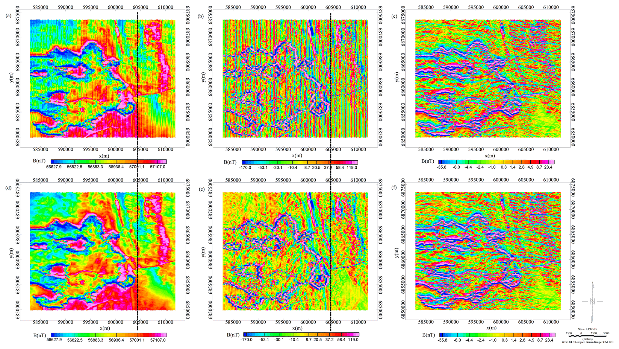
Figure 1The directional property of leveling error. (a) The raw magnetic data. (b) The horizontal gradients of the raw magnetic data. (c) The vertical gradients of the raw magnetic data. (d) The leveled magnetic data. (e) The horizontal gradients of the leveled magnetic data. (f) The vertical gradients of the leveled magnetic data.
Figure 2 depicts the maximum values of the horizontal gradients and the vertical gradients. We find the horizontal gradients are not a smooth trend and has an amplitude jump at the black dotted line in Fig. 2a. To analyze the amplitude variety, two black dotted lines are given at the corresponding position in Fig. 1. The comprehensive analysis indicates that the larger amplitudes in the horizontal gradients are caused by the discontinuous abnormal distribution on the left side of the survey area. The vertical gradient amplitudes are affected by the same reason as shown in Fig. 2b. That is to say, the anomaly data show a non-negligible discontinuity in flight line direction and the tie-line direction.
As mentioned in the Introduction, many previous papers are based on the assumption that the geophysical field is continuous, but the leveling errors are not continuous between adjacent flight lines. The leveling errors mainly contribute to the difference between adjacent flight lines. However, a neglected issue is that the discontinuity of the anomaly may be regarded as leveling errors, which have a considerable impact on the data leveling. A corresponding simulation experiment has proved this thought and been published in our papers (Zhu et al., 2020; Zhang et al., 2021). Therefore, reasonable leveling preprocessing is needed to filter anomaly data and construct a smooth field to level data accurately.
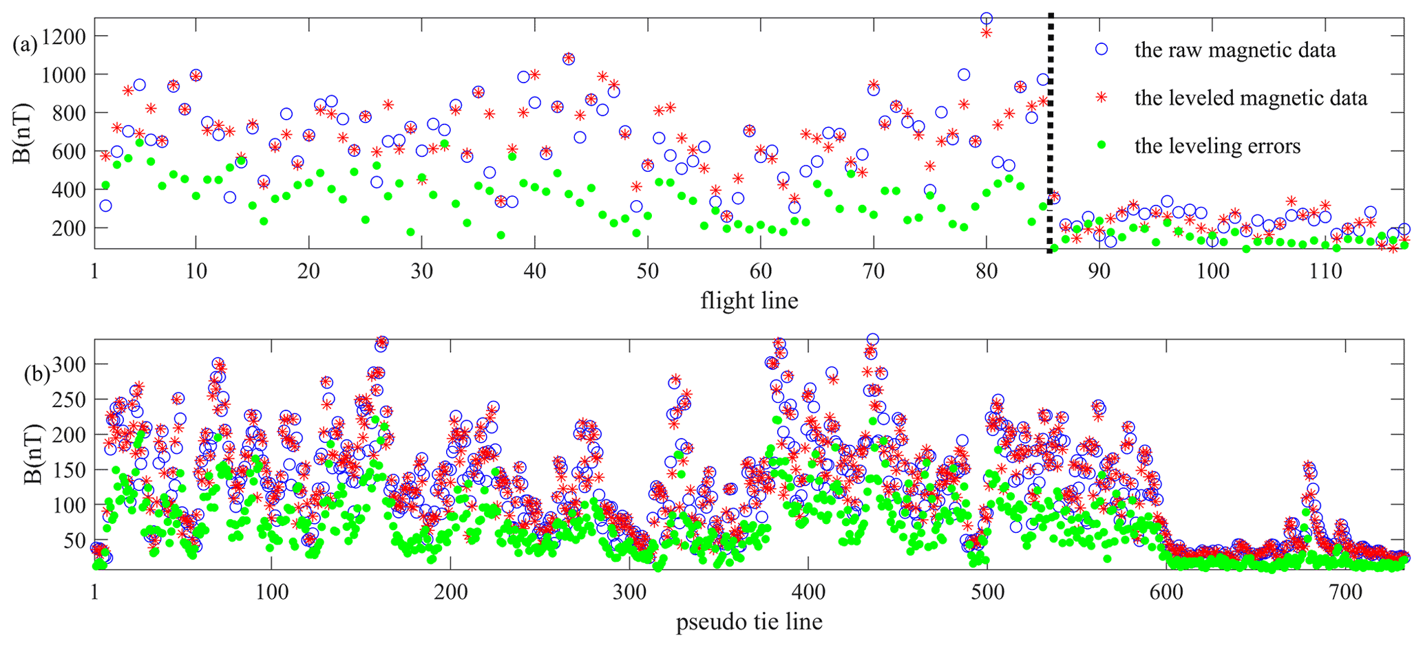
Figure 2The maximum values of the gradients. (a) The horizontal gradients. (b) The vertical gradients.
3.1 Leveling preprocessing
As the property analysis of leveling errors, leveling preprocessing is needed to remove the survey anomaly in the leveling processing. The vertical gradient of the raw data could better represent the anomaly distribution as shown in Fig. 1c. Then, the smooth field is constructed based on the vertical gradient data. We can distinguish the anomaly points by a comprehensive comparison between the flight line and tie-line directions. If the vertical gradient of the survey point data is greater than the average values of its flight line or tie-line directions following Eq. (2), the survey point is deemed a potential anomaly.
where is the vertical gradient of the ith survey data in the jth flight line. Then, the potential anomaly point is replaced by the average level of the flight line following Eq. (3).
After processing the area point to point, a smooth field DP is constructed without the potential anomaly point. The smooth dataset can better represent the real data level compared with the raw data.
3.2 Unidirectional variational model
Following leveling preprocessing, a new leveling method is proposed based on the unidirectional variational model and the spatially adaptive multi-scale model. As with the leveling error properties discussed above, the leveling error shows a similar directional distribution property to the stripe noise in imaging systems. It is feasible to separate the leveling error components and the pure geophysical data in the destriping process.
In the image processing field, the geometric variation method and partial differential equation (PDE) display excellent results which make comprehensive use of functional analysis, variation calculation, partial differential equations, differential geometry, vector and tensor analysis, bounded variation space, and viscosity solution theory (Osher and Rudin, 1990; Liu et al., 2016). Here we consider the survey data to be a 2D function defined in a bounded domain Ω, and the leveling error is an additive drift formulated as
where DP(i,j) is the preprocessed data of the ith survey data in the jth flight line, E(i,j) is the leveling error trend of the survey point and R(i,j) is the residual data. The ill-posed problems require introducing a regularizing constraint on the solution. Combining with prior information, an estimate of the leveling error trend can be computed by minimizing an energy functional that includes a penalty term and a regularization term. The penalty term is used to keep the fidelity of the estimated solution to the preprocessed data. And the regularization term can regulate the smoothness of the solution.
In an energy functional framework, Rudin et al. (1992) introduced the total variation (TV) norm and proposed the ROF (Rudin, Osher and Fatemi) total variation, model which has been widely used in image-denoising applications. The energy functional is defined as
where λ is the regularization coefficient that quantifies the degree of smoothness and TV(E) is the total variation in the estimated solution E expressed as
The ROF model can better preserve discontinuities in the solution, which is important for geophysical data processing.
By exploiting the unidirectional signature of stripes in the TV framework, Bouali and Ladjal (2011) proposed the unidirectional variational model, which provides optimal qualitative and quantitative results on images contaminated with severe stripes. The scholars have studied the algorithm in detail and applied it to the stripe noise removal (Huang et al., 2016; Zhang and Zhang, 2016; Liu et al., 2019). Based on a directional distribution property, leveling error trend E can be viewed as a similarly structured variable, variations of which are mainly concentrated along the x axis. In mathematical words, the leveling errors of most survey points have the following property:
Integration of Eq. (7) over the survey area leads the inequality to a characteristic of the leveling error:
where TVx and TVy are horizontal and vertical variations. To obtain a robust leveling error removal, the leveling error characteristic is introduced into the energy functional in Eq. (5):
Then, the minimization of the unidirectional variational model in Eq. (9) is calculated by the alternating direction method of multipliers (ADMM) in a sequence of iterative sub-optimizations (Bertsekas, 1982). Based on the directional distribution of the leveling error, the unidirectional variational model separates the leveling error trend and the residual data into the penalty term and the regularization term which can better constraint the decomposition results.
3.3 Spatially adaptive multi-scale variation
In the unidirectional variational method, the regularization coefficient λ has to be assigned carefully because the regularization coefficient has a deciding effect on the smoothness of the results. A large regularization coefficient will produce an unfavorable over-smoothing effect. That is, excessive geologic information is decomposed to leveling error trend. If the regularization coefficient is too small, the stripes cannot be extracted completely. Based on the multi-scale hierarchical decomposition theory (Tadmor et al., 2003), we add the spatially adaptive multi-scale model to the energy functional to avoid the difficulty in the selection of the regularization coefficient. While the preprocessed data are decomposed as leveling errors E and residual data R, the algorithm loops through multiple iterations in multi-scale regularization coefficients to retain more useful details. In the kth iteration, the energy functional is expressed as
In order to accurately decompose leveling errors, the regularization coefficient is updated with a spatially adaptive strategy. The calculated resulting data at each iteration are further decomposed into smaller regularization coefficients. When the iteration has converged as shown in Eq. (11), the algorithm terminates the iterative decomposition.
The raw input data are decomposed as a multi-residual dataset and a leveling error trend in Eq. (12):
The leveled data Dl are calculated by removing the directional stripe trend Ek from the geophysical data D.
The spatially adaptive multi-scale model can level geophysical data automatically and avoid the unfavorable over-smoothing effect.
4.1 Airborne electromagnetic data leveling
We have tested the proposed leveling method on the AEM data collected by the Ontario Geological Survey, Ministry of Northern Development and Mines (MNDM). The survey was carried out in the North Spirit Lake area using the time-domain GEOTEM® 1000 electromagnetic system mounted on a fixed wing platform (Ontario Geological Survey, 2007). The area data, named Geophysical Data Set 1056, were flown with a 200 m flight line spacing. And the flight line direction is 40–220∘. The B-field data of serial flight lines L10510 to L11150 at the ninth channel are shown in Fig. 3a and are affected by the obviously inconsistent data level among the flight lines.
After leveling preprocessing, Fig. 3b presents the constructed smooth field, which has filtered most of the potential anomaly points. It is worth mentioning that the altitude sensitivity in the AEM data should be reduced before leveling (Huang, 2008). Based on the superposed dipole assumption (Fraser, 1972), Huang (2008) proposed transforming the altitude-sensitive AEM data into the response-parameter domain. Following the opinion of Huang, we transformed the AEM data used in the paper into response-parameter domain data. Figure 3c depicts the processed data by the unidirectional variational model algorithm in which the initial regularization coefficient λ0 is fixed to 50 and updated with in iteration. The proposed leveling processing can be completed automatically without professional geophysicists.
In contrast, Fig. 3d presents the data processed by Fugro Airborne Surveys through multiple steps, including lag adjustment, drift adjustments, spike editing for spherical events, the correction for coherent noise and adaptive filtering. The drift adjustment used is in flight form based on the baseline minimum rule along each channel (Ontario Geological Survey, 2007). Through a graphic screen display, the flight lines are passed through a low-order polynomial function to correct drift.
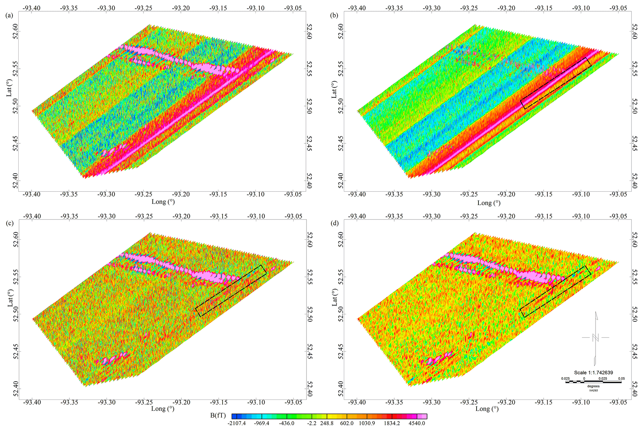
Figure 3The AEM data leveling. (a) Raw AEM data. (b) The preprocessed smooth field. (c) Leveled data by the unidirectional variational model algorithm. (d) The data processed by Fugro Airborne Surveys.
Figure 4 shows the leveled transient data to compare the results in greater detail. Two flight lines are selected and locally enlarged to show leveling errors in different degrees, as Fig. 4b and c show. The leveling errors are approximately zero in the 25th flight line, and the level errors are larger in the 50th flight line. Both leveling methods can remove the leveling errors in the area. Because of extra denoising by Fugro Airborne Surveys, the processed data show some differences, especially in the spike of anomaly points.
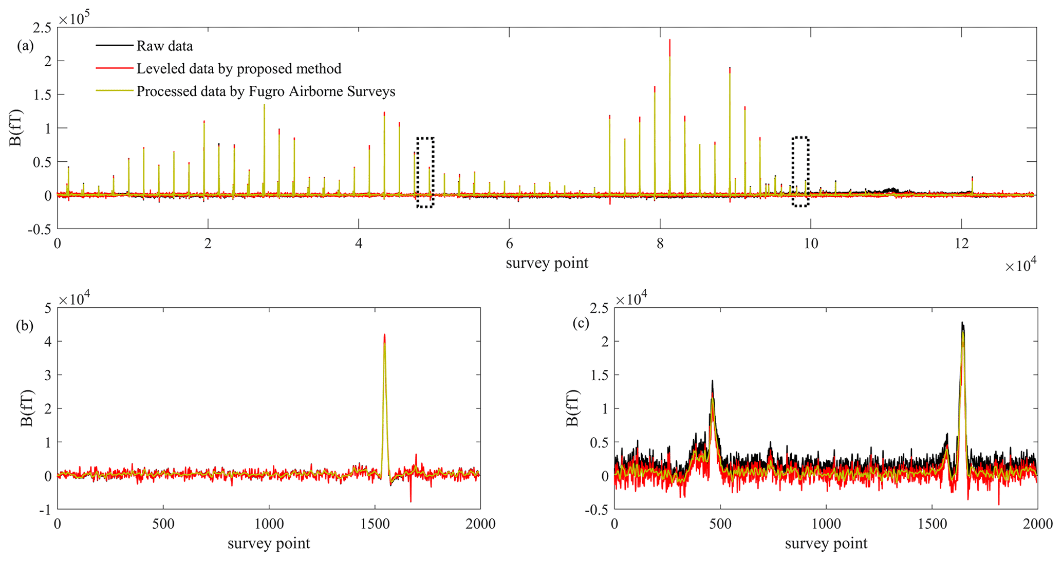
Figure 4The result comparison analysis between the unidirectional variational model algorithm and Fugro Airborne Surveys. (a) All flight line data. (b) The 25th flight line data, corresponding to the first black dotted rectangle in (a). (c) The 50th flight line data, corresponding to the second black dotted rectangle in (a).
4.2 Airborne magnetic data leveling
We have tested the proposed leveling method on the magnetic data collected by the Ontario Airborne Geophysical Survey as shown in Fig. 1a. The dataset information has been provided in the image space property analysis. Based on the vertical gradient of the survey area, we removed the anomaly points that may interfere with the leveling. As Fig. 5a shows, the constructed smooth field could better represent the data level of the measuring area. In the leveling process, the parameters of the unidirectional variational model algorithm are set in the same way as the AEM data leveling example. That is, the initial regularization coefficient λ0 is fixed to 50 and reduced by half in each iteration. The leveled data and decomposed leveling errors are shown in Fig. 5b and c.
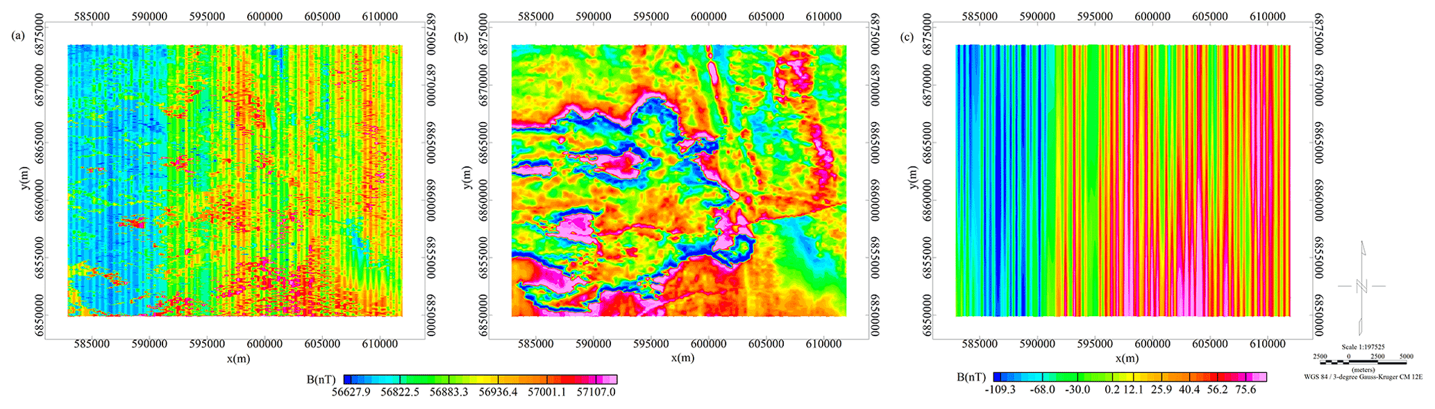
Figure 5The leveling of the magnetic data. (a) The preprocessed smooth field. (b) Leveled data by the unidirectional variational model algorithm. The figure is shown with the same color bar as the leveling results in Fig. 1d. (c) Decomposed leveling errors.
The data leveled by the tie-line leveling method are used as comparative data, which have been given in Fig. 1d. Then, contrasts between the corrected transient data are presented in Fig. 6. Similarly, we enlarged two flight lines in different error degrees as the samples, as Fig. 6b and c show. The leveling errors are larger in the 44th flight line and are approximately zero in the 112nd flight line.
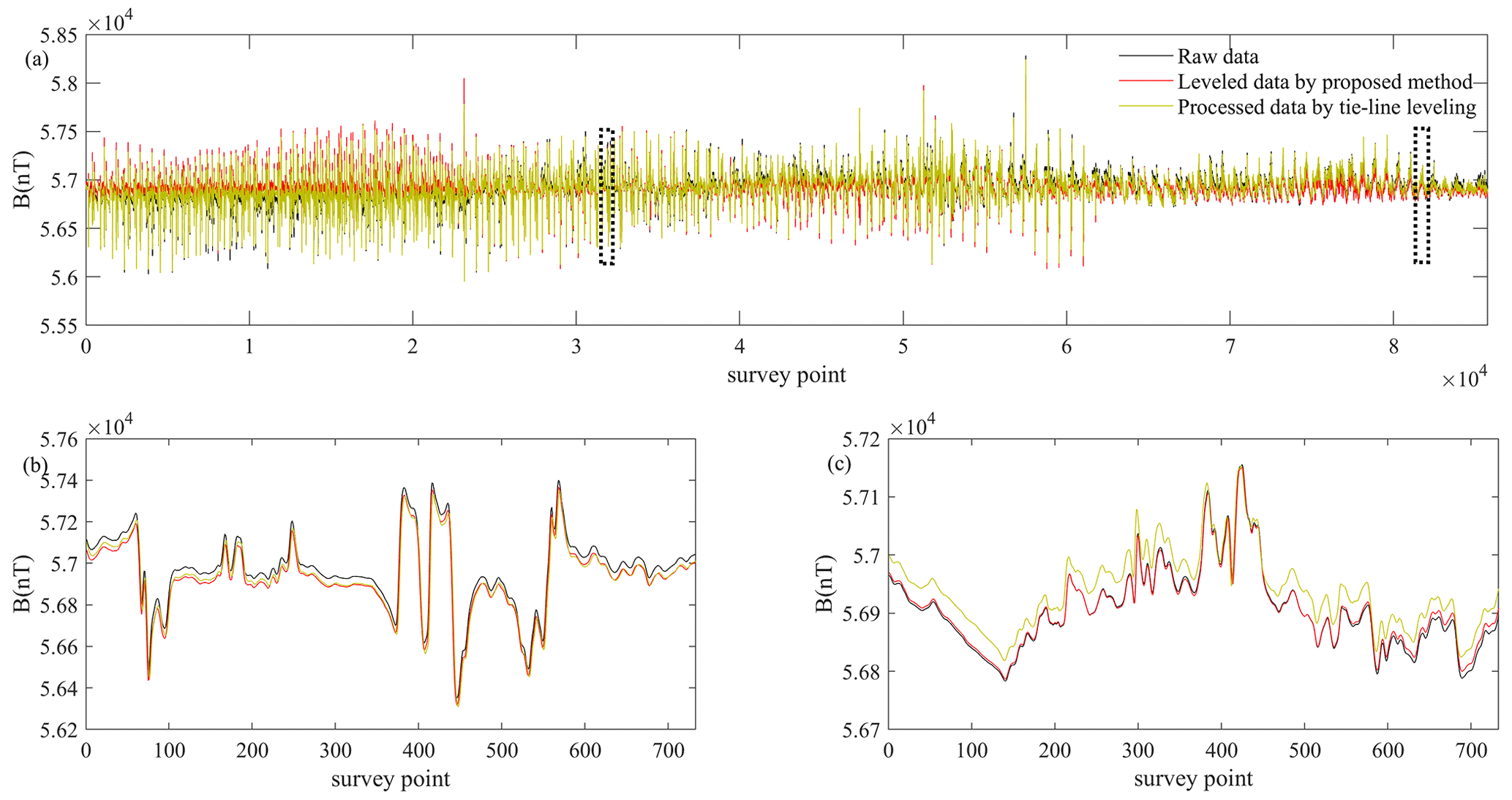
Figure 6Leveled magnetic data. (a) All flight line data. (b) The 44th flight line data, corresponding to the first black dotted rectangle in (a). (c) The 112nd flight line data, corresponding to the second black dotted rectangle in (a).
4.3 Apparent-conductivity data leveling
The third example shows leveling results for apparent-conductivity data. Geotech Ltd. carried out a helicopter-borne combined aeromagnetic and electromagnetic survey for the Ministry of Northern Development and Mines in 2014 which is performed as part of the Ontario Geological Survey geoscience program in the Nestor Falls area in northwestern Ontario. In the helicopter-borne electromagnetic survey, the geophysical surveys used the versatile time-domain electromagnetic (VTEM®Plus) system with Z-component measurements. Based on the resistivity depth imaging (RDI) technique (Meju, 1998), Geotech Ltd. converted the electromagnetic profile decay data into an equivalent resistivity versus depth cross section, by deconvolution of the measured electromagnetic data. Data compilation and processing were carried out using Geosoft® OASIS montaj™ operated by Geotech Ltd. (Ontario Geological Survey, 2014).
The dataset used in the paper is formed by 71 flight lines named L310 to L1000 as a part of Geophysical Data Set 1076 measured in the surveys. Figure 7a presents the apparent conductivity calculated from the response at 97 m average depth from the surface. There are obvious striped errors along the flight line direction.
According to the length of flight lines, the survey area data are divided into two parts in the leveling example. We applied the same parameters to test the robustness of the unidirectional variational model algorithm. The regularization coefficient is fixed to 50 in the initial iteration and reduced by half at each iteration. The leveled data and decomposed leveling errors are shown in Fig. 7b and c. The contrast of the corrected transient data is presented in Fig. 8. We selected and enlarged two flight lines in different error degrees as the samples, as Fig. 8b and c show. The leveling errors are larger in the sixth flight line and approximately zero in the 71st flight line.

Figure 7The leveling of the apparent-conductivity data. (a) The raw data. (b) Leveled data by the unidirectional variational model algorithm. (c) Decomposed leveling errors.
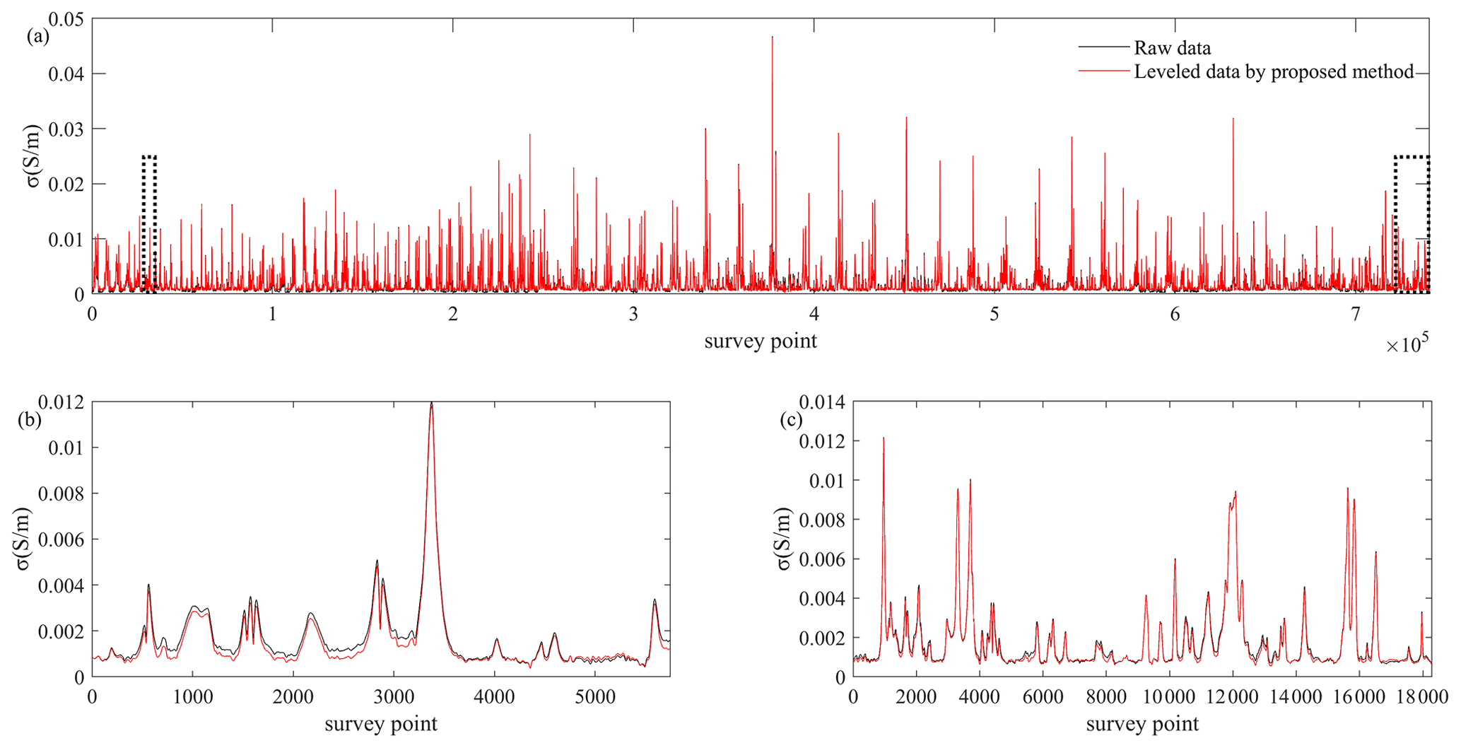
Figure 8Leveled apparent-conductivity data. (a) All flight line data. (b) The sixth flight line data, corresponding to the first black dotted rectangle in (a). (c) The 71st flight line data, corresponding to the second black dotted rectangle in (a).
Firstly, we analyzed and discussed the leveling results in the AEM example. As shown in Fig. 3, the leveling errors in the AEM data are associated with a block of flight lines and presented as a block distribution. Based on the proposed leveling method, the first step is leveling preprocessing to filter the survey anomaly in the field. The preprocessing is essential to accurately distinguish the data level in the following processing. As shown in Fig. 9a, a common phenomenon is that the maximum value in one flight line is greater than the median value and average value in the flight line. For certain flight lines, the maximum value is even thousands of times greater than the median value and average value which have been tested in Fig. 9b. The anomaly data with large amplitude may hide the real data level. The leveling preprocessing solved the problem by removing the potential anomaly point and constructing a smooth field. And the smooth field can better reflect the real data level by comparing the data in Fig. 3a and b.
Then, a unidirectional variational model is applied to the smooth field, taking into account the directional distribution property discussed above. The variations in leveling errors are mainly concentrated along the tie-line direction compared with the flight line direction. Meanwhile, spatially adaptive multi-scale variation is introduced to assist the parameter selection. This is very important for the massive data processing in geophysical exploration. Fully automatic data processing not only accelerates the processing speed but also reduces the process steps of data processors.
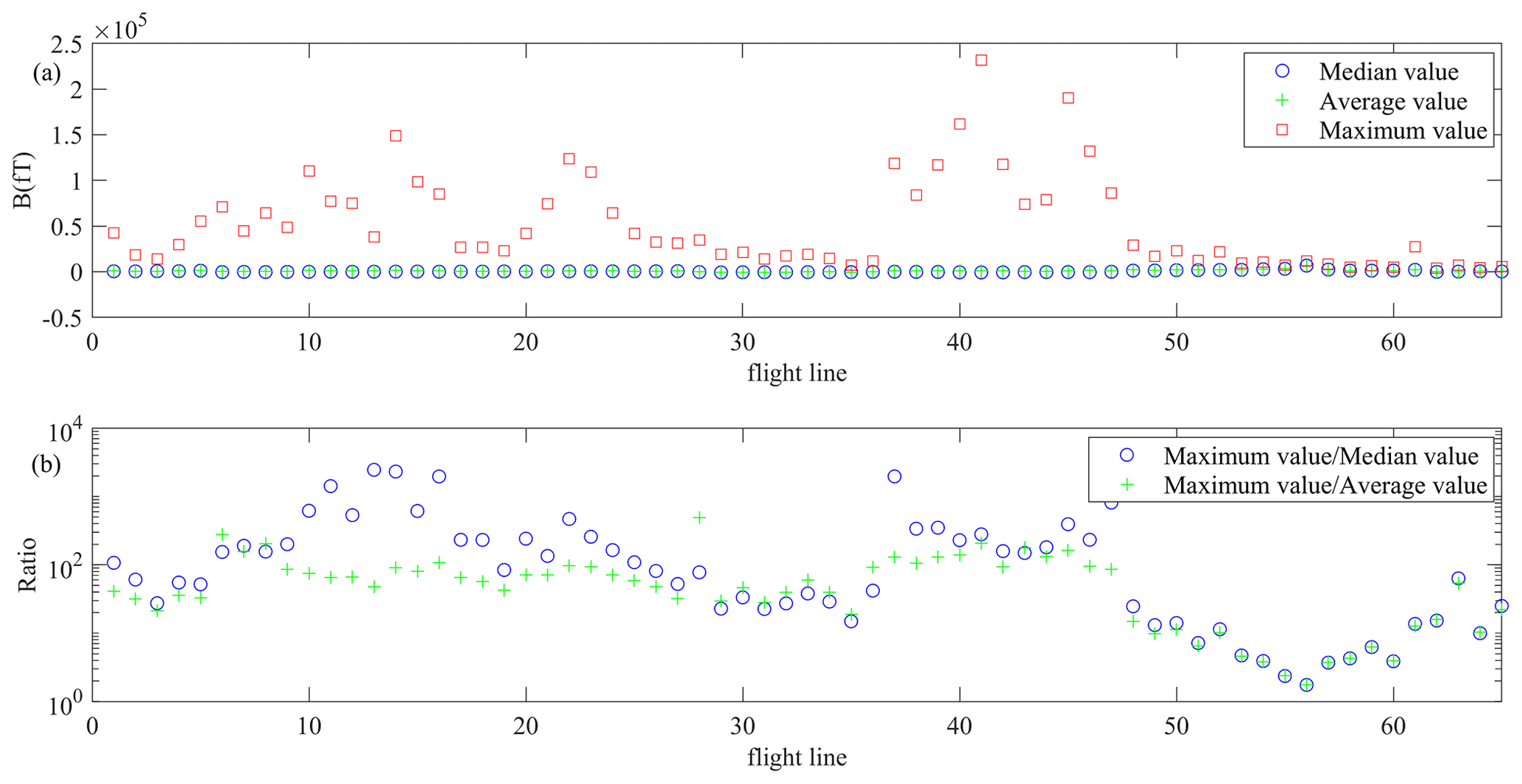
Figure 9Statistical values of the raw AEM data. (a) The median value, average value and maximum value of each flight line in the field. (b) The ratio of the maximum value to the median value and of the maximum value to the average value. For a better visualization effect, the ratio curves are shown in logarithmic form.
Figures 3 and 4 compare the leveling results of the proposed method and Fugro Airborne Surveys. Both leveling methods can remove the leveling errors and obtain smooth leveled data. Meanwhile, the amplitude and area of anomaly data were almost unchanged. The conclusion can be confirmed by the transient data curves in Fig. 4. That is, the proposed leveling method can reach an ideal process result in a relatively simple and completely automated way.
It is worth noting that most leveling methods cannot distinguish between the leveling errors and the anomaly throughout the flight lines. As Fig. 3c shows, there is a narrow strip of anomaly in the black dotted rectangle. If the narrow strip is long enough throughout the flight line, it will be misjudged as leveling errors. The problem may appear in most leveling methods. The leveling preprocessing used in this paper can avoid the problem by separating the anomaly data in advance. The anomaly data are not involved in the leveling process, which protects the integrity of the anomaly data to the greatest extent.
We analyzed the leveled results in the leveling examples of magnetic data and apparent-conductivity data in a similar way. Compared with AEM data example, there are more anomaly areas in a scattered or continuous distribution form as Figs. 1a and 7a show. When we applied leveling preprocessing to the datasets and removed suspected anomaly points, the leveling errors are underlined in the constructed smooth field as shown in Fig. 5a. This is helpful to check and operate the leveling errors. In the following leveling steps, we used fixed algorithm parameters in the unidirectional variational model and spatially adaptive multi-scale variation algorithms. Figures 5–8 intuitively show the leveled data in maps and transient data curves.
In the airborne magnetic example, the comparison shows that both the tie-line leveling method and the proposed leveling method work well in removing leveling errors as Figs. 1d and 5b show. In reality, the tie-line leveling method regards tie-line data as standard and depends highly on the data quality of measured tie lines. There are usually uncontrollable differences in measurement environment when flight lines and tie lines are flown, which increases the disturbance in tie-line leveling. The relevant professionals are needed to operate the leveling steps. However, the proposed leveling method can achieve an expected result in a relatively general way, despite the data type and the source of leveling errors.
The leveled data of an apparent-conductivity example are given in Fig. 7. In the survey area, the lengths of flight lines have larger difference. In order to decompose the survey data, an extra division is needed according to the lengths of flight lines so that the leveled areas are relatively regular in the image space domain. From the view of leveled data in Figs. 7b and 8a, we can roughly estimate that the leveled data are at a consistent data level.
In this paper, we proposed a leveling method based on a unidirectional variational model and a spatially adaptive multi-scale model. A reasonable leveling preprocessing is introduced to highlight the real data level, which helps to extract the leveling error component. Based on the vertical gradient data, a simple filtering is used to remove the large-amplitude anomaly data. As the field examples show, leveling preprocessing has two advantages in the leveling method. One, the leveling preprocessing reduces the obstacle to distinguish leveling errors. Second, it is helpful to ensure the integrity of anomaly data, including the anomaly amplitude and anomaly area.
Then, a general leveling method is proposed considering the directional distribution property and amplitude variety property of the leveling error. The leveling method combines a unidirectional variational model with a spatially adaptive multi-scale model. The proposed leveling method is an adaptive and automatic correction without tie-line data which can produce desired results with stability and robustness. Geophysical explorations have vast amounts of measured data which increase the requirement to research automatic processing methods. In the leveling method, the survey data are leveled as a whole rather than through block processing. Integrated processing avoids the regional error caused by strong noise, missing data or error transfer in the common leveling process. We have confirmed the reliability of the method by applying it to the AEM, magnetic data and apparent-conductivity data with fixed parameters and without tie-line control.
The data used in the paper have been made available by the Ontario Geological Survey (Geophysical Data Set 1056: http://www.geologyontario.mndm.gov.on.ca/mndmaccess/mndm_dir.asp?type=pub&id=GDS1056a, Ontario Geological Survey, 2007; Geophysical Data Set 1076: http://www.geologyontario.mndm.gov.on.ca/mndmaccess/mndm_dir.asp?type=pub&id=GDS1076, Ontario Geological Survey, 2014). More information can be found on the official website (https://www.mndm.gov.on.ca/en, last access: 20 April 2022).
The paper is approved by all authors for publication. QZ and CS developed the algorithm model and performed the simulations. FY designed the experiments and CL carried them out. YL prepared the paper with contributions from all co-authors.
The contact author has declared that neither they nor their co-authors have any competing interests.
Publisher's note: Copernicus Publications remains neutral with regard to jurisdictional claims in published maps and institutional affiliations.
We all thank the Ontario Geological Survey for permission to use the geophysical data in this study. Moreover, the authors are appreciative of Jean M. Legault, Chief Geophysicist of Geotech Ltd., for providing us with access to Geophysical Data Set 1076. We also appreciate the positive and constructive comments and suggestions on our paper from the editor and the reviewers.
This study was supported by the Jilin Province Science and Technology Development Plan (“Research on airborne electromagnetic data leveling technology based on total variational model (YDZJ202101ZYTS064)”).
This paper was edited by Lev Eppelbaum and reviewed by two anonymous referees.
Bandy, W. L., Gangi, A. F., and Morgan, F. D.: Direct method for determining constant corrections to geophysical survey lines for reducing mis-tie, Geophysics, 55, 885–896, https://doi.org/10.1190/1.1442903, 1990.
Beiki, M., Bastani, M., and Pedersen, L. B.: Leveling HEM and aeromagnetic data using differential polynomial fitting, Geophysics, 75, 13–23, https://doi.org/10.1190/1.3279792, 2010.
Bertsekas, D. P.: Constrained optimization and Lagrange Multiplier methods, Computer Science and Applied Mathematics, Academic, Boston, MA, USA, ISBN 1886529043, 1982.
Bouali, M. and Ladjal, S.: Toward optimal destriping of MODIS data using a unidirectional variational model, IEEE T. Geosci. Remote, 49, 2924–2935, https://doi.org/10.1109/TGRS.2011.2119399, 2011.
Davydenko, A. Y. and Grayver, A. V.: Principal component analysis for filtering and leveling of geophysical data, J. Appl. Geophys., 109, 266–280, https://doi.org/10.1016/j.jappgeo.2014.08.006, 2014.
Eppelbaum, L. V. and Mishne, A. R.: Unmanned Airborne Magnetic and VLF investigations: Effective Geophysical Methodology of the Near Future, Positioning, 2, 112–133, https://doi.org/10.4236/pos.2011.23012, 2011.
Fan, Z. F., Huang, L., Zhang, X. J., and Fang, G. Y.: An elaborately designed virtual frame to level aeromagnetic data, IEEE Geosci. Remote S., 13, 1153–1157, https://doi.org/10.1109/LGRS.2016.2574750, 2016.
Ferraccioli, F., Gambetta, M., and Bozzo, E.: Microlevelling procedures applied to regional aeromagnetic data: an example from the Transantarctic Mountains, Geophys. Prospect., 46, 177–196, https://doi.org/10.1046/j.1365-2478.1998.00080.x, 1998.
Foster, M. R., Jines, W. R., and Weg, K. V.: Statistical estimation of systematic errors at intersections of lines of aeromagnetic survey data, J. Geophys. Res., 75, 1507–1511, https://doi.org/10.1029/JB075i008p01507, 1970.
Fraser, D. C.: A new multicoil aerial electromagnetic prospecting system, Geophysics, 37, 518–537, https://doi.org/10.1190/1.1440277, 1972.
Gao, L. Q., Yin, C. C., Wang, N., Liu, Y. H., Su, Y., and Xiong, B.: Leveling of airborne electromagnetic data based on curvelet transform, Chin. J. Geophys., 5, 1785–1796, 2021.
Green, A.: Correcting drift errors in HEM data, ASEG Special Publications, 2, 1, https://doi.org/10.1071/aseg2003ab058, 2003.
Groune, D., Allek, K., and Bouguern, A.: Statistical approach for microleveling of aerophysical data, J. Appl. Geophys., 159, 418–428, https://doi.org/10.1016/j.jappgeo.2018.09.023, 2018.
Hood, P.: History of Aeromagnetic Survey in Canada, The Leading Edge, 26, 1384–1392, https://doi.org/10.1190/1.2805759, 2007.
Huang, H. P.: Airborne geophysical data leveling based on line-to-line correlations, Geophysics, 73, 83–89, https://doi.org/10.1190/1.2836674, 2008.
Huang, H. P. and Fraser, D. C.: Airborne resistivity data leveling, Geophysics, 64, 378–385, https://doi.org/10.1190/1.1444542, 1999.
Huang, Y. Z., He, C., Fang, H. Z., and Wang, X. P.: Iteratively reweighted unidirectional variational model for stripe non-uniformity correction, Infrared Phys. Techn., 75, 107–116, https://doi.org/10.1016/j.infrared.2015.12.030, 2016.
Ishihara, T.: A new leveling method without the direct use of crossover data and its application in marine magnetic surveys, weighted spatial averaging and temporal filtering, Earth Planets Space, 67, 11, https://doi.org/10.1186/s40623-015-0181-7, 2015.
Liu, C. J., Zhou, H. L., and Qian, X.: Imaging processing geometric variational and multiscale method, Tsinghua University Press, ISBN 9787302433194, 2016.
Liu, L., Xu, L. P., and Fang, H. Z.: Simultaneous Intensity Bias Estimation and Stripe Noise Removal in Infrared Images Using the Global and Local Sparsity Constraints, IEEE T. Geosci. Remote, 58, 1777–1789, https://doi.org/10.1109/TGRS.2019.2948601, 2019.
Luo, Y., Wand, P., Duan, S. L., and Cheng, H. D.: Leveling total field aeromagnetic data with measured vertical gradient, Chin. J. Geophys., 55, 3854–3861, 2012.
Luyendyk, A. P. J.: Processing of airborne magnetic data, AGSO Journal of Australian Geology and Geophysics, 17, 31–38, 1997.
Mauring, E. and Kihle, O.: Leveling aerogeophysical data using a moving differential median filter, Geophysics, 71, 5–11, https://doi.org/10.1190/1.2163912, 2006.
Mauring, E., Beard, L. P., and Kihle, O.: A comparison of aeromagnetic levelling techniques with an introduction to median leveling, Geophys. Prospect., 50, 43–54, https://doi.org/10.1046/j.1365-2478.2002.00300.x, 2002.
Meju, M. A.: Short Note: A simple method of transient electromagnetic data analysis, Geophysics, 63, 405–410, https://doi.org/10.1190/1.1444340, 1998.
Minty, B. R. S.: Simple micro-levelling for aeromagnetic data, Explor. Geophys., 22, 591–592, https://doi.org/10.1071/eg991591, 1991.
Nelson, J. B.: Leveling total-field aeromagnetic data with measured horizontal gradients, Geophysics, 59, 1166–1170, https://doi.org/10.1190/1.1443673, 1994.
Ontario Geological Survey: Ontario airborne geophysical surveys, magnetic and electromagnetic data, North Spirit Lake area, Geophysical Data Set 1056, Ontario Geological Survey [data set], http://www.geologyontario.mndm.gov.on.ca/mndmaccess/mndm_dir.asp?type=pub&id=GDS1056a (last access: 20 April 2022), 2007.
Ontario Geological Survey: Ontario airborne geophysical surveys, magnetic and electromagnetic data, grid and profile data (ASCII and Geosoft® formats) and vector data, Nestor Falls area, Geophysical Data Set 1076, Ontario Geological Survey [data set], http://www.geologyontario.mndm.gov.on.ca/mndmaccess/mndm_dir.asp?type=pub&id=GDS1076 (last access: 20 April 2022), 2014.
Osher, S. and Rudin, L. I.: Feature oriented image enhancement using shock filters, SIAM J. Numer. Anal., 27, 919–940, https://resolver.caltech.edu/CaltechCSTR:1989.cs-tr-89-03 (last access: 25 April 2022), 1990.
Rudin, L. I., Osher, S., and Fatemi, E.: Nonlinear total variation based noise removal algorithms, Physica D, 60, 259–268, https://doi.org/10.1016/0167-2789(92)90242-F, 1992.
Siemon, B.: Levelling of helicopter-borne frequency-domain electromagnetic data, J. Appl. Geophys., 67, 206–218, https://doi.org/10.1016/j.jappgeo.2007.11.001, 2009.
Srimanee, C., Dumrongchai, P., and Duangdee, N.: Airborne gravity data adjustment using a cross-over adjustment with constraints, International Journal of Geoinformatics, 16, 51–60, 2020.
Tadmor, E., Nezzar, S., and Vese, L.: A multiscale image representation using hierarchical, Multiscale Model. Sim., 2, 554–579, https://doi.org/10.1137/030600448, 2003.
Tezkan, B., Stoll, J. B., Bergers, R., and Grossbach, H.: Unmanned aircraft system proves itself as a geophysical measuring platform for aeromagnetic surveys, First Break, 29, 103–105, 2011.
Urquhart, T.: Decorrugation of enhanced magnetic field maps, SEG Technical Program Expanded Abstracts, Society of Explor. Geophys., 371–372, https://doi.org/10.1190/1.1892383, 1988.
Valleau, N. C.: HEM data processing – A practical overview, Explor. Geophys., 31, 584–594, https://doi.org/10.1071/eg00584, 2000.
White, J. C. and Beamish, D.: Levelling aeromagnetic survey data without the need for tie-lines, Geophys. Prospect., 63, 451–460, https://doi.org/10.1111/1365-2478.12198, 2015.
Yarger, H. L., Robertson, R. R., and Wentland, R. L.: Diurnal drift removal from aeromagnetic data using least squares, Geophysics, 43, 1148–1156, https://doi.org/10.1190/1.1440884, 1978.
Yin, C. C. and Fraser, D. C.: Attitude corrections of helicopter EM data using a superposed dipole model, Geophysics, 69, 431–439, https://doi.org/10.1190/1.1707063, 2004.
Zhang, Q., Peng, C., Lu, Y. M., Wang, H., and Zhu, K. G.: Airborne electromagnetic data levelling using principal component analysis based on flight line difference, J. Appl. Geophys., 151, 290–297, https://doi.org/10.1016/j.jappgeo.2018.02.023, 2018.
Zhang, Q., Yan, F., and Liu, Y. Q.: Airborne geophysical data levelling based on variational mode decomposition, Near Surf. Geophys., 19, 377–394, https://doi.org/10.1002/nsg.12138, 2021.
Zhang, Y. Z. and Zhang, T. X.: Structure-guided unidirectional variation de-striping in the infrared bands of MODIS and hyperspectral images, Infrared Phys. Tech., 77, 132–143, https://doi.org/10.1016/j.infrared.2016.05.022, 2016.
Zhu, K. G., Zhang, Q., Peng, C., Wang, H., and Lu, Y. M.: Airborne electromagnetic data levelling based on inequality-constrained polynomial fitting, Explor. Geophys., 51, 600–608, 2020.