the Creative Commons Attribution 4.0 License.
the Creative Commons Attribution 4.0 License.
 | 21 Oct 2022
Accuracies of field CO2–H2O data from open-path eddy-covariance flux systems: assessment based on atmospheric physics and biological environment
Xinhua Zhou
Bai Yang
Yanlei Li
Fengyuan Yu
Tala Awada
Jiaojun Zhu
Ecosystem CO2–H2O data measured by infrared gas analyzers in open-path eddy-covariance (OPEC) systems have numerous applications, such as estimations of CO2 and H2O fluxes in the atmospheric boundary layer. To assess the applicability of the data for these estimations, data uncertainties from analyzer measurements are needed. The uncertainties are sourced from the analyzers in zero drift, gain drift, cross-sensitivity, and precision variability. These four uncertainty sources are individually specified for analyzer performance, but so far no methodology exists yet to combine these individual sources into a composite uncertainty for the specification of an overall accuracy, which is ultimately needed. Using the methodology for closed-path eddy-covariance systems, this overall accuracy for OPEC systems is determined from all individual uncertainties via an accuracy model and further formulated into CO2 and H2O accuracy equations. Based on atmospheric physics and the biological environment, for EC150 infrared CO2–H2O analyzers, these equations are used to evaluate CO2 accuracy (±1.22 mgCO2 m−3, relatively ±0.19 %) and H2O accuracy (±0.10 gH2O m−3, relatively ±0.18 % in saturated air at 35 ∘C and 101.325 kPa). Both accuracies are applied to conceptual models addressing their roles in uncertainty analyses for CO2 and H2O fluxes. For the high-frequency air temperature derived from H2O density along with sonic temperature and atmospheric pressure, the role of H2O accuracy in its uncertainty is similarly addressed. Among the four uncertainty sources, cross-sensitivity and precision variability are minor, although unavoidable, uncertainties, whereas zero drift and gain drift are major uncertainties but are minimizable via corresponding zero and span procedures during field maintenance. The accuracy equations provide rationales to assess and guide the procedures. For the atmospheric background CO2 concentration, CO2 zero and CO2 span procedures can narrow the CO2 accuracy range by 40 %, from ±1.22 to ±0.72 mgCO2 m−3. In hot and humid weather, H2O gain drift potentially adds more to the H2O measurement uncertainty, which requires more attention. If H2O zero and H2O span procedures can be performed practically from 5 to 35 ∘C, the H2O accuracy can be improved by at least 30 %: from ±0.10 to ±0.07 gH2O m−3. Under freezing conditions, the H2O span procedure is impractical but can be neglected because of its trivial contributions to the overall uncertainty. However, the zero procedure for H2O, along with CO2, is imperative as an operational and efficient option under these conditions to minimize H2O measurement uncertainty.
- Article
(913 KB) - Full-text XML
- BibTeX
- EndNote


Open-path eddy-covariance (OPEC) systems are used most in quantity to measure boundary-layer CO2, H2O, heat, and momentum fluxes between ecosystems and the atmosphere (Lee and Massman, 2011). For flux measurements, an OPEC system is equipped with a fast-response three-dimensional (3-D) sonic anemometer, to measure 3-D wind velocities and sonic temperature (Ts), and a fast-response infrared CO2–H2O analyzer (hereafter referred to as an infrared analyzer or analyzer) to measure CO2 and H2O concentrations or densities (Fig. 1). In this system, the analyzer is adjacent to the sonic measurement volume. Both anemometer and analyzer together provide synchronized high-frequency (e.g., 10 to 20 Hz) measurements, which are used to compute the fluxes at a location represented by the measurement volume (Aubinet et al., 2012). Given that the measurement conditions, which are spatially homogenous in flux sources/sinks and temporally steady in turbulent flows without advection, satisfy the underlying theory for eddy-covariance flux techniques (Katul et al., 2004; Finnigan, 2008), the quality of each flux data point primarily depends on the exactness of field measurements of the variables, such as CO2, H2O, Ts, and 3-D wind, at the sensor sensing scales (Foken et al., 2012; Richardson et al., 2012), although the quality may also be degraded by other biases if not fully corrected. In an OPEC system, other biases are commonly sourced from the tilt of the vertical axis of the sonic anemometer away from the vertical vector of natural wind (Kaimal and Haugen, 1969), the spatial separation between the anemometer and the analyzer (Laubach and McNaughton, 1998), the line and/or volume averaging of measurements (Wyngaard, 1971; Andreas, 1981), the response delay of sensors to fluctuations in measured variables (Horst, 2000), the air density fluctuations due to heat and water vapor transfer (Webb et al., 1980), and the filtering in data processing (Rannik and Vesala, 1999). These biases are theoretically correctable through coordinate rotation corrections for the tilt (Tanner and Thurtell, 1969; Wilczak et al., 2001); covariance lag maximization for the separation (Moncrieff et al., 1997; Ibrom et al., 2007); low- and high-frequency corrections for the data filtering, line and/or volume averaging, and response delay (Moore, 1986; Lenschow et al., 1994; Massman, 2000; van Dijk, 2002); and Webb–Pearman–Leuning (WPL) corrections for the air density fluctuations (Webb et al., 1980). Even though these corrections are thorough for corresponding biases, errors in the ultimate flux data still exist due to uncertainties related to measurement exactness at the sensor sensing scales (Fratini et al., 2014; Zhou et al., 2018). These uncertainties are not only unavoidable because of actual or apparent instrumental drifts due to the thermal sensitivity of sensor path lengths, long-term aging of sensor detection components, and unexpected factors in field operations (Fratini et al., 2014), but they are also not mathematically correctable because their sign and magnitude are unknown (Richardson et al., 2012). The overall measurement exactness related to these uncertainties would be a valuable addition to flux data analysis (Goulden et al., 1996; Anthoni et al., 2004).

Figure 1Integration of an EC150 infrared CO2–H2O analyzer for CO2 density () and H2O density () with a CSAT3A sonic anemometer for three-dimensional (3-D) wind velocities and sonic temperature (Ts) in an open-path eddy-covariance flux system (Image credit: Campbell Scientific Inc., UT, USA).
In addition to flux computations, the data for individual variables from these field measurements can be important in numerous applications. Knowledge of measurement exactness is also required for an accurate assessment of data applicability (Csavina et al., 2017; Hill et al., 2017). The infrared analyzer in an OPEC system outputs CO2 density ( in mgCO2 m−3) and H2O density ( in gH2O m−3). For instance, , along with Ts and atmospheric pressure (P), can be used to derive ambient high-frequency air temperature (Ta) (Swiatek, 2018). In this case, given an exact equation of Ta in terms of the three independent variables , Ts, and P, the applicability of this equation to the OPEC systems for Ta depends wholly on the measurement exactness of the three independent variables. The higher the degree of exactness, the less uncertain the Ta. The assessment of the applicability necessitates the knowledge of the measurement exactness. In reality, to the best of our knowledge, neither the overall measurement exactness of from the infrared analyzers nor the exactness of Ts from the sonic anemometers (Larry Jecobsen, personal communication, 2022) is available. This study defines and estimates the measurement exactness of including from infrared analyzers through the consolidation of the measurement uncertainties, which are not practically avoidable or mathematically correctable, although they can be minimized through analyzer maintenance.
As comprehensively reviewed by Richardson et al. (2012), numerous previous studies including Goulden et al. (1996), Lee et al. (1999), Anthoni et al. (1999, 2004), and Flanagan and Johnson (2005) have quantified various sources of flux measurement errors and have attempted to attach confidence intervals to the annual sums of net ecosystem exchange. These sources include measurement methods (e.g., sensor separation and site homogeneity; Munger et al., 2012), data processing algorithms (e.g., data filtering, Rannik and Vesala, 1999, and data gap filling, Richardson and Hollinger, 2007), measurement conditions (e.g., advection; Finnigan, 2008), energy closure (Foken, 2008), and sensor body heating effects (Burba et al., 2008). Instead of quantifying the flux errors, Foken et al. (2004, 2012) assessed the flux data quality and divided it into nine grades (1 to 9) based on steady state, turbulence conditions, and wind direction in the sonic anemometer coordinate system. The lower the grade, the smaller the error in flux data (i.e., higher flux data quality); the higher grade, the greater the error in flux data (i.e., lower flux data quality). This grade matrix (Foken et al., 2004, 2012) has been adopted by AmeriFlux (2018) for their flux data quality assessments. To correct the measurement biases from infrared analyzers, Burba et al. (2008) developed a correction method for sensor body heating effects on CO2 and H2O fluxes, whereas Fratini et al. (2014) developed a method for correcting the raw high-frequency CO2 and H2O data using the interpolated zero and span coefficients of an infrared analyzer from the analyzer maintenance such as zero and span procedures under the same conditions but at the beginning and ending of each maintenance period. The corrected data were then used to re-estimate the fluxes. Nevertheless, no study so far has addressed the overall measurement exactness of or , which are related to the unavoidable and uncorrectable measurement uncertainties in the CO2 and H2O data from the infrared analyzers in OPEC systems, even though this overall measurement exactness is fundamental for data analysis in applications (Richardson et al., 2012). Therefore, instead for the overall exactness of an individual field CO2 or H2O measurement, the infrared analyzers are specified only for their individual CO2 and H2O measurement uncertainties sourced from their zero and gain drifts, cross-sensitivity to background , and measurement precision variability (LI-COR Biosciences, 2021c; Campbell Scientific Inc., 2021b).
For any sensor, the measurement exactness depends on its performance as commonly specified in terms of accuracy, precision, and other uncertainty descriptors such as sensor hysteresis. Conventionally, accuracy is defined as a systematic uncertainty, while precision is defined as a random measurement error (ISO, 2012, where ISO is the acronym of International Organization for Standardization). Other uncertainty descriptors are also defined for specific reliabilities in instrumental performance. For example, CO2 zero drift is one of the descriptors specified for the performance of infrared analyzers in CO2 measurements (Campbell Scientific Inc., 2021b). Both accuracy and precision are universally applicable to any sensor for the specification of its performance in measurement exactness. Other uncertainty descriptors are more sensor-specific (e.g., cross-sensitivity to is used for infrared analyzers in OPEC and CPEC systems, where CPEC is an acronym for closed-path eddy covariance).
Conventionally, sensor accuracy is the degree of closeness to which its measurements are to the true value in the measured variable; sensor precision, related to repeatability, is the degree to which repeated measurements under unchanged conditions produce the same values (Joint Committee for Guides in Metrology, 2008). Another definition advanced by the ISO (2012), revising the conventional definition of accuracy as trueness originally representing only systematic uncertainty, specifies accuracy as a combination of both trueness and precision. An advantage of this definition for accuracy is the consolidation of all measurement uncertainties. According to this definition, the accuracy is the range of composited uncertainty from all uncertainty sources in field measurements. For CPEC systems, Zhou et al. (2021) developed a method and derived a model to assess the accuracy of mixing ratio measurements of infrared analyzers. Their model was further formulated as a set of equations to evaluate the defined accuracies for CO2 and H2O mixing ratio data from CPEC systems. Although the CPEC systems are very different from OPEC systems in their structural designs (e.g., measurements take place inside a closed cuvette vs. in an open space) and in output variables (e.g., mixing ratio vs. density), similarities exist between the two systems in measurement uncertainties as specified by their manufacturers (Campbell Scientific Inc., 2021a, b) because the infrared analyzers in both systems use the same physics theories and similar optical techniques for their measurements (LI-COR Biosciences, 2021b, c). Accordingly, the method developed by Zhou et al. (2021) for CPEC systems can be reasonably applied to their OPEC counterparts with rederivation of the model and reformulation of equations. Following the methodology of Zhou et al. (2021) and using the specifications of EC150 infrared analyzers in OPEC systems as an example (Campbell Scientific Inc., 2021b), we can derive the model and formulate equations to assess the accuracies of CO2 and H2O measurements by infrared analyzers in OPEC systems; discuss the usage of accuracies in flux analysis, data applications, and analyzer field maintenance; and ultimately provide a reference for the flux measurement community in order to specify the overall accuracy of field measurements by infrared analyzers in OPEC systems.
An OPEC system for this study includes, but is not limited to, a CSAT3A sonic anemometer and an EC150 infrared analyzer (Fig. 1). The system operates in a Ta range from −30 to 50 ∘C and in a P range from 70 to 106 kPa. Within these operational ranges, the specifications for CO2 and H2O measurements (Campbell Scientific Inc., 2021b) are given in Table 1.
Table 1Measurement specifications for EC150 infrared CO2–H2O analyzers (Campbell Scientific Inc., UT, USA).
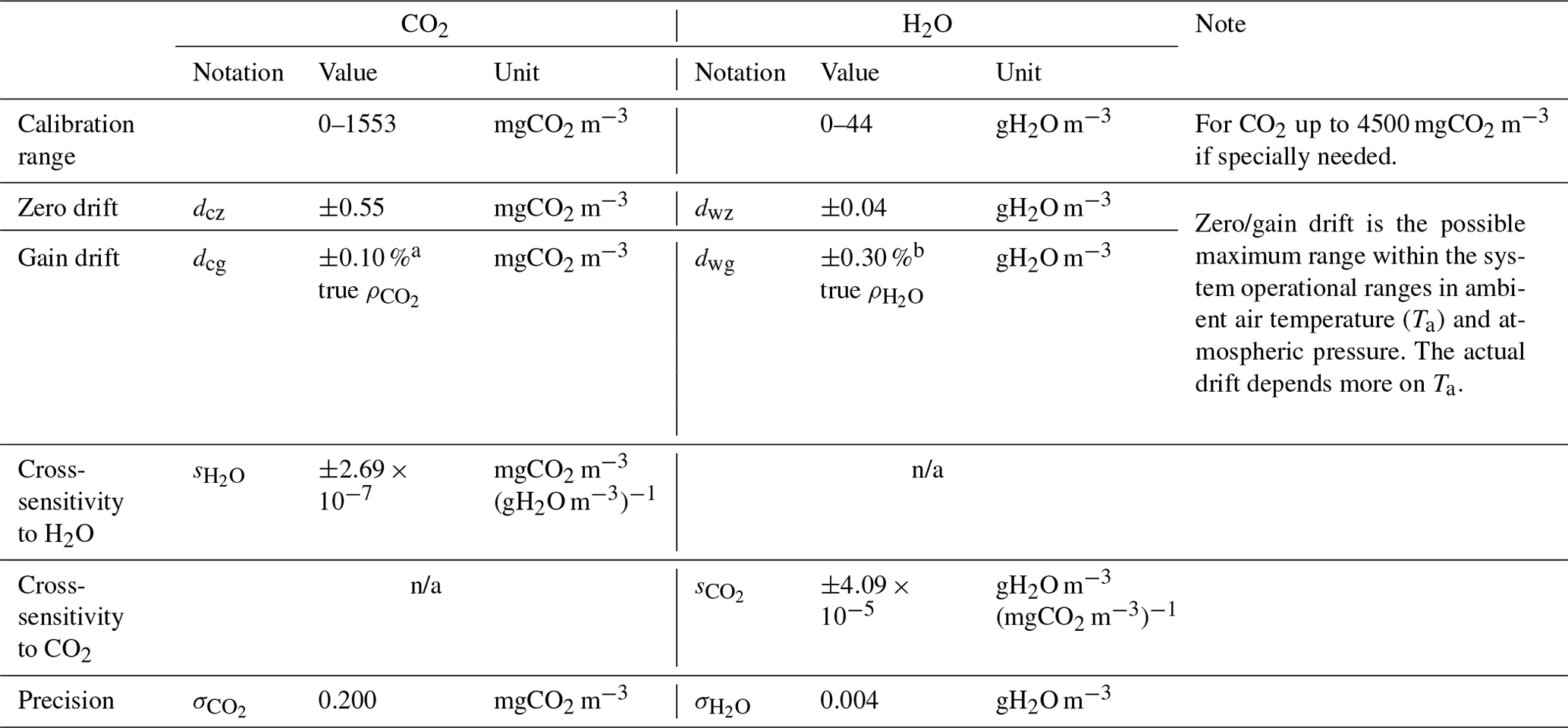
a 0.10 % is the CO2 gain drift percentage denoted by in the text, and is CO2 density. b 0.30 % is the H2O gain drift percentage denoted by in the text, and is H2O density. n/a denotes “not applicable”.
In Table 1, the top limit of 1553 mgCO2 m−3 in the calibration range for CO2 density in dry air is more than double the atmospheric background CO2 density of 767 mgCO2 m−3, or 419 µmolCO2 mol−1, where mol is the unit for dry air, reported by the Global Monitoring Laboratory (2022) with a Ta of 20 ∘C under a P of 101.325 kPa (i.e., normal temperature and pressure, Wright et al., 2003). The top limit of 44 gH2O m−3 in the calibration range for H2O density is equivalent to a 37 ∘C dew point, higher than the highest 35 ∘C dew point ever recorded under natural conditions on Earth (National Weather Service, 2022).
The measurement uncertainties from infrared analyzers for CO2 and H2O in Table 1 are specified by individual uncertainty components along with their magnitudes: zero drift, gain drift, cross-sensitivity to , and precision variability. Zero drift uncertainty is an analyzer non-zero response to zero air/gas (i.e., air/gas free of CO2 and H2O). Gain drift uncertainty is an analyzer trend-deviation response to a measured gas species away from its true value in proportion (Campbell Scientific Inc., 2021b). Cross-sensitivity is an analyzer response to either background CO2 if H2O is measured or background H2O if CO2 is measured. Precision variability is an analyzer random response to minor unexpected factors. For CO2 and H2O, these four components should be composited as an overall uncertainty in order to evaluate the accuracy, which is ultimately needed in practice.
Precision variability is a random error, and the other specifications can be regarded as trueness. Zero drifts are primarily impacted by Ta, and so are gain drifts (see the “Note” column in Table 1 and also Fratini et al., 2014). Additionally, each gain drift is also positively proportional to the true magnitude of density (i.e., true or true ) under measurements. Lastly, cross-sensitivity to is related to the background amount of as indicated by its units: mgCO2 m−3 (gH2O m−3)−1 for CO2 measurements and gH2O m−3 (mgCO2 m−3)−1 for H2O measurements.
Accordingly, beyond statistical analysis, the accuracy of measurements should be evaluated over a Ta range of −30 to 50 ∘C, a range of up to 44 gH2O m−3, and a range of up to 1553 mgCO2 m−3.
The measurement accuracy of infrared analyzers is the possible maximum range of overall measurement uncertainty from the four uncertainty sources as specified in Table 1: zero drift, gain drift, cross-sensitivity, and precision variability. The four uncertainties interactionally or independently contribute to the overall uncertainty in a measured value. Given the true α density (ραT, where subscript α can be either CO2 or H2O) and measured α density (ρα), the difference between the true and measured α densities (Δρα) is given by
The analyzer overestimates the true value if Δρα>0, exactly estimates the true value if Δρα=0, and underestimates the true value if Δρα<0. The measurement accuracy is the maximum range of Δρα (i.e., an accuracy range). According to the analyses of Zhou et al. (2021) for CPEC infrared analyzers, as mathematically shown in Appendix A, this range is interactionally contributed by the zero drift uncertainty (), gain drift uncertainty (), and cross-sensitivity uncertainty () along with an independent addition from the precision uncertainty (). However, any interactional contribution from a pair of uncertainties is 3 orders smaller in magnitude than each individual contribution in the pair. The contribution to the accuracy range due to interactions can be reasonably neglected. Therefore, the accuracy range can be simply modeled as a sum of the absolute values of the four component uncertainties. From Eq. (A7) in Appendix A, the measurement accuracy of α density from OPEC systems by infrared analyzers is defined in an accuracy model as
Assessment of the accuracy of field CO2 or H2O measurements is, by the use of known and/or estimable variables, the formulation and evaluation of the four terms on the right side of this accuracy model.
Based on accuracy Model (2), we define the accuracy of field CO2 measurements from OPEC systems by infrared analyzers () as
where is CO2 zero drift uncertainty, is CO2 gain drift uncertainty, is cross-sensitivity-to-H2O uncertainty, and is CO2 precision uncertainty.
CO2 precision () is the standard deviation of random errors among repeated measurements under the same conditions (Joint Committee for Guides in Metrology, 2008). The random errors generally have a normal statistical distribution (Hoel, 1984). Therefore, using this deviation, the precision uncertainty for an individual CO2 measurement at a 95 % confidence interval (P value of 0.05) can be statistically formulated as
The other uncertainties, due to CO2 zero drift, CO2 gain drift, and cross-sensitivity to H2O, are caused by the inability of the working equation inside the analyzer operating system (OS) to adapt to the changes in analyzer-internal and ambient environmental conditions, such as internal housing CO2 and/or H2O levels and ambient air temperature. From the derivations in the “Theory and operation” section in LI-COR Biosciences (2001, 2021b, c), a general model of the working equation for is given by
where subscripts c and w indicate CO2 and H2O, respectively; aci (i=1, 2, 3, 4, or 5) is a coefficient of the 5-order polynomial for the terms inside curly brackets; Acs and Aws are the power values of analyzer source lights at the chosen wavelengths for CO2 and H2O measurements, respectively; Ac and Aw are their respective remaining power values after the source lights pass through the measured air sample; Sw is cross-sensitivity of the detector to H2O while detecting CO2, at the wavelength for CO2 measurements (hereafter referred to as sensitivity to H2O); Zc is the CO2 zero adjustment (i.e., CO2 zero coefficient); and Gc is the CO2 gain adjustment (i.e., commonly known as the CO2 span coefficient). For an individual analyzer, the parameters aci, Zc, Gc, and Sw in Model (5) are statistically estimated in the production calibration against a series of standard CO2 gases at different concentration levels over the ranges of and P (hereafter referred to as calibration). Since the estimated parameters are specific for the analyzer, Model (5) with these estimated parameters becomes an analyzer-specific CO2 working equation. The working equation is used internally by the infrared analyzer to compute as the closet proxy for true from field measurements of Ac, Acs, Aw, Aws, and P.
The analyzer-specific working equation is deemed to be accurate immediately after the calibration through estimations of aci, Zc, Gc, and Sw in production, while Zc and Gc can be re-estimated in the field (LI-COR Biosciences, 2021c). However, as used internally by an optical instrument under changing environments vastly different from its calibration conditions by its manufacturer, the working equation may not be fully adaptable to the changes, which might be reflected through CO2 zero and/or gain drifts of the deployed infrared analyzer. In the working equation for from Model (5), the parameter Zc is related to CO2 zero drift; Gc to CO2 gain drift; and Sw to sensitivity to H2O. Therefore, the analyses of Zc and Gc, along with Sw, aid in understanding the causes of CO2 zero drift, CO2 gain drift, and sensitivity to H2O. Such understanding is necessary to formulate , , and in Model (3).
4.1 Zc and (CO2 zero drift uncertainty)
In production, an infrared analyzer is calibrated for zero air/gas to report zero plus an unavoidable random error. However, when using the analyzer in measurement environments that are different from calibration conditions, the analyzer often reports this zero , while exposed to zero air, as a value that migrates gradually away from zero and possibly beyond , which is known as CO2 zero drift. This drift is primarily affected by a combination of three factors: (i) the temperature surrounding the analyzer away from the calibration temperature, (ii) traceable CO2 and H2O accumulations, such as during use, inside the analyzer light housing due to an inevitable, although small, leaking exchange of housing air with the ambient air (hereafter referred to as housing CO2–H2O accumulation), and (iii) aging of analyzer components (Richardson et al., 2012).
Firstly, the dependency of analyzer CO2 zero drift on ambient air temperature arises due to a thermal expansion/contraction of analyzer components that slightly changes the analyzer geometry (Fratini et al., 2014). This change in geometry can deviate the light path length for measurement a little away from the length under manufacturer calibration, contributing to the drift. Additionally, inside an analyzer, the performance of the light source and absorption detector for measurement, as well as the electronic components for measurement control, can vary slightly with temperature. In production, an analyzer is calibrated to compensate for the ensemble of such dependencies as assessed in a calibration chamber. The compensation algorithms are implemented in the analyzer OS, which is kept as proprietary by the analyzer manufacturer. However, the response of an analyzer to a temperature varies as conditions change over time (Fratini et al., 2014). Therefore, manufacturers typically specify an expected range of typical or maximal drift per ∘C (see Table 1 and also see the section for analyzer specifications in Campbell Scientific Inc., 2021b). Secondly, the housing CO2–H2O accumulation is caused by unavoidable small leaks in the light housing of an infrared analyzer. The housing is technically sealed to keep housing air close to zero air by introducing scrubber chemicals into the housing to absorb any CO2 and H2O that may sneak into the housing through an exchange with any ambient air (LI-COR Biosciences, 2021c). Over time, the scrubber chemicals may be saturated by CO2 and/or H2O or lose their active absorbing effectiveness, which can result in housing CO2–H2O accumulations. Thirdly, as optical components, the light source may gradually become dim, and the absorption detector may gradually become less sensitive. The accumulation and aging develop slowly and less obviously in the relatively long term (e.g., months or longer), whereas the dependencies of drift on ambient air temperature can occur quickly and more clearly as soon as an analyzer is deployed in the field (Richardson et al., 2012). Apparently, the drift with ambient air temperature is a major concern if an analyzer is maintained as scheduled by its manufacturer for the replacement of scrubber chemicals (Campbell Scientific Inc., 2021b).
Due to the CO2 zero drift, the working equation needs to be adjusted through its parameter re-estimation to adapt the ambient air temperature near which the system is running, housing CO2–H2O accumulation, and analyzer component aging. This adjustment technique is the zero procedure, which brings the and in zero air/gas measurement back to zero as closely as possible. In this section, our discussion focuses on CO2, and the same application to H2O will be described in the following sections. In the field, the zero procedure should be feasibly operational using one air/gas benchmark to re-estimate one parameter in the working equation. This parameter must be adjustable to output zero from the zero air/gas benchmark. By setting the left side of Model (5) to zero and rearranging it, it is clear that Zc is such a parameter that can be adjusted to result in a zero value for zero air/gas:
where Ac0 and Aw0 are the counterparts of Ac and Aw for zero air/gas, respectively. For an analyzer, the zero procedure for CO2 is thus to re-estimate Zc in balance of Eq. (6).
If Zc could continually balance Eq. (6) after the zero procedure, the CO2 zero drift would not be significant; however, this is not the case. Similar to its performance after the manufacturer calibration, an analyzer may still drift after the zero procedures due to frequent changes in ambient air temperature, housing CO2–H2O accumulation, and/or analyzer component age. Nevertheless, the Zc value needed for an analyzer to be punctually adaptable for these changes is unpredictable because these changes are not foreseeable. Assuming on-schedule maintenance (i.e., the scrubber chemicals inside the analyzer light housing are replaced following the manufacturer's guidelines), the housing CO2–H2O accumulation should not be a concern. While the ambient temperature surrounding the infrared analyzer is not controlled, the CO2 zero drift is therefore mainly influenced by Ta and can be ±0.55 mgCO2 m−3 at most within the operational ranges in Ta and P for the EC150 infrared analyzers in OPEC systems (Table 1).
Given that an analyzer performs best almost without zero drift at the ambient air temperature for the calibration/zeroing procedure (Tc) and that it possibly drifts while Ta gradually changes away from Tc, then the further away Ta is from Tc, the more it possibly drifts in the CO2 zero. Over the operational range in P of the EC150 infrared analyzers used for OPEC systems, this drift is more proportional to the difference between Ta and Tc but is still within the specifications (Campbell Scientific Inc., 2021b). Accordingly, CO2 zero drift uncertainty at Ta can be formulated as
where, over the operational range in Ta of EC150 infrared analyzers used for OPEC systems, Trh is the highest-end value (50 ∘C) and Trl is the lowest-end value (−30 ∘C, Table 1). from this equation has the maximum range, as specified in Table 1, equal to dcz in magnitude as if Ta and Tc were separately at the two ends of operational range in Ta of OPEC systems.
4.2 Gc and (CO2 gain drift uncertainty)
An infrared analyzer was also calibrated against a series of standard CO2 gases. The calibration sets the working equation from Model (5) to closely follow the gain trend of change in . As was determined with the zero drift, the analyzer, with changes in housing CO2–H2O accumulation, ambient conditions, and age during its deployment, could report CO2 gradually drifting away from the real gain trend of the change in , which is specifically termed CO2 gain drift. This drift is affected by almost the same factors as the CO2 zero drift (Richardson et al., 2012; Fratini et al., 2014; LI-COR Biosciences, 2021c).
Due to the gain drift, the infrared analyzer needs to be further adjusted, after the zero procedure, to tune its working equation back to the real gain trend in of measured air as closely as possible. This is done with the CO2 span procedure. This procedure can be performed through use of either one or two span gases (LI-COR Biosciences, 2021c). If two are used, one span gas is slightly below the ambient CO2 density and the other is at a much higher density to fully cover the CO2 density range by the working equation. However, commonly, like the zero procedure, this procedure is simplified by the use of one CO2 span gas, as a benchmark, with a known CO2 density () around the typical CO2 density values in the measurement environment. If one CO2 span gas is used, only one parameter in the working equation is available for adjustment. Weighing the gain of the working equation more than any other parameter, this parameter is the CO2 span coefficient (Gc) (see Model 5). The CO2 span gas is used to re-estimate Gc to satisfy the following equation (for details, see LI-COR Biosciences, 2021c):
Similar to the zero drift, the CO2 gain drift continues after the CO2 span procedure. Based on a similar consideration for the specifications of CO2 zero drift, the CO2 gain drift is specified by the maximum CO2 gain drift percentage ( %) associated with as ±0.10 % × (true ) (Table 1). This specification is the maximum range of CO2 measurement uncertainty due to the CO2 gain drift within the operational ranges in Ta and P of the EC150 infrared analyzers in OPEC systems.
Given that an analyzer performs best, almost without gain drift, at the ambient air temperature for calibration/span procedures (also denoted by Tc because zero and span procedures should be performed under similar ambient air temperature conditions) but also drifts while Ta gradually changes away from Tc, then the further away Ta is from Tc, the greater potential that the analyzer drifts. Accordingly, the same approach to the formulation of CO2 zero drift uncertainty can be applied to the formulation of the approximate equation for CO2 gain drift uncertainty at Ta as
where is the true CO2 density unknown in measurement. Given that the measured value of CO2 density is represented by , by referencing Eq. (1), can be expressed as
The terms inside the parentheses in this equation are the measurement uncertainties for that are smaller in magnitude, by at least 2 orders, than , whose magnitude in atmospheric background under the normal temperature and pressure as used by Wright et al. (2003) is 767 mgCO2 m−3 (Global Monitoring Laboratory, 2022). Therefore, in Eq. (10) is the best alternative, with the greatest likelihood, to for the application of Eq. (9). As such, in Eq. (9) can be reasonably approximated by for equation applications. Using this approximation, Eq. (9) becomes
With being measured, this equation is applicable in estimating the CO2 gain drift uncertainty. The gain drift uncertainty () from this equation has the maximum range of , as if Ta and Tc were separately at the two ends of operational range in Ta of OPEC systems. With the greatest likelihood, this maximum range is the closest to × (true ) as specified in Table 1.
4.3 Sw and (sensitivity-to-H2O uncertainty)
The infrared wavelength of 4.3 µm for CO2 measurements is minorly absorbed by H2O (LI-COR Biosciences, 2021c; Campbell Scientific Inc., 2021b). This minor absorption slightly interferes with the absorption by CO2 in the wavelength (McDermitt et al., 1993). The power of the same measurement light (i.e., Acs as a steady value in the CO2 working equation from Model 5) through several gas samples with the same CO2 density, but different backgrounds of H2O densities, is detected with different values of Ac in the working equation from Model (5). Without parameter Sw and its joined term in the working equation, different Ac values must result in significantly different values, although they are actually the same. In case of the same CO2 density in the airflows under different H2O backgrounds, the different values of Ac to report similar are accounted for by Sw associated with Aw and Aws in the working equation from Model (5). Similar to Zc and Gc in the CO2 working equation, Sw is not perfectly accurate and can have uncertainty in the determination of . This uncertainty for EC150 infrared analyzers is specified by sensitivity to H2O () as mgCO2 m−3 (gH2O m−3)−1 (Table 1). As indicated by its unit, this uncertainty is linearly related to . Assuming the analyzer for CO2 works best, without this uncertainty, in dry air, could be formulated as
where 44 gH2O m−3, as addressed in Sect. 2, is the top limit of H2O density measurements. Accordingly, can be in the range of
4.4 (CO2 measurement accuracy)
Substituting Eqs. (4), (7), (11), and (13) into Model (3), for an individual CO2 measurement from OPEC systems by infrared analyzers can be expressed as
This is the CO2 accuracy equation for the infrared analyzers within OPEC systems. It expresses the accuracy of a field CO2 measurement from the OPEC systems in terms of the analyzer specifications , , dcz, , and the OPEC system operational range in Ta as indicated by Trh and Trl, measured variables and Ta, and a known variable Tc. Given the specifications and the known variable, this equation can be used to evaluate the CO2 accuracy as a range in relation to Ta and .
4.5 Evaluation of
Given the analyzer specifications, the accuracy of field CO2 measurements from an infrared analyzer after calibration, zero, and/or span at Tc can be evaluated using the CO2 accuracy Eq. (14) over a domain of Ta and . To visualize the relationship of accuracy with Ta and , the accuracy is presented better as the ordinate along the abscissa of Ta for at different levels and must be evaluated within possible maximum ranges of Ta and in ecosystems. In evaluation, the Ta is limited to the −30 to 50 ∘C range within which EC150 infrared analyzers used for OPEC systems operate, Tc can be assumed to be 20 ∘C (i.e., standard air temperature as used by Wright et al., 2003), and can range according to its variation in ecosystems.
4.5.1 range
The upper measurement limit of CO2 density by the infrared analyzers can reach up to 1553 mgCO2 m−3. In the atmosphere, its background CO2 mixing ratio is currently 419 µmolCO2 mol−1 (Global Monitoring Laboratory, 2022). Under normal temperature and pressure conditions (Wright et al., 2003), this background mixing ratio is equivalent to 767 mgCO2 m−3 in dry air. The CO2 density in ecosystems commonly ranges from 650 to 1500 mgCO2 m−3 (LI-COR Biosciences, 2021c), depending on biological processes (Wang et al., 2016), aerodynamic regimes (Yang et al., 2007), and thermodynamic states (Ohkubo et al., 2008). In this study, this range is extended from 600 to 1600 mgCO2 m−3 as a common range within which is evaluated. Because of the dependence of on (Eq. 14), to show the accuracy at different CO2 levels, the range is further divided into five grades of 600, 767 (atmospheric background), 1000, 1300, and 1600 mgCO2 m−3 for evaluation presentations as in Fig. 2.
According to a brief review by Zhou et al. (2021) on the plant physiological threshold in air temperature for growth and development and the soil temperature dynamic related to CO2 from microorganism respiration and/or wildlife activities in terrestrial ecosystems, at any grade of 1000, 1300, or 1600 mgCO2 m−3 should, at 5 ∘C, start to converge asymptotically to the atmospheric CO2 background (767 mgCO2 m−3 at −30 ∘C, Fig. 2). Without an asymptotical function for the convergence curve, conservatively assuming the convergence has a simple linear trend with Ta from 5 to −30 ∘C, is evaluated up to the magnitude of along the trend (Fig. 2).
4.5.2 range
At Ta=Tc, the CO2 accuracy is best at its narrowest range to be the sum of precision and sensitivity-to-H2O uncertainties (±0.39 mgCO2 m−3). However, away from Tc, its range near-linearly becomes wider. The range can be summarized as ±0.40 to ±1.22 mgCO2 m−3 over the domain of Ta and (Fig. 2a and CO2 columns in Table 2). The maximum CO2 relative accuracy at the different levels of is in a range of ±0.07 % at 1600 mgCO2 m−3 to 0.19 % at 600 mgCO2 m−3 (from data for Fig. 2b).
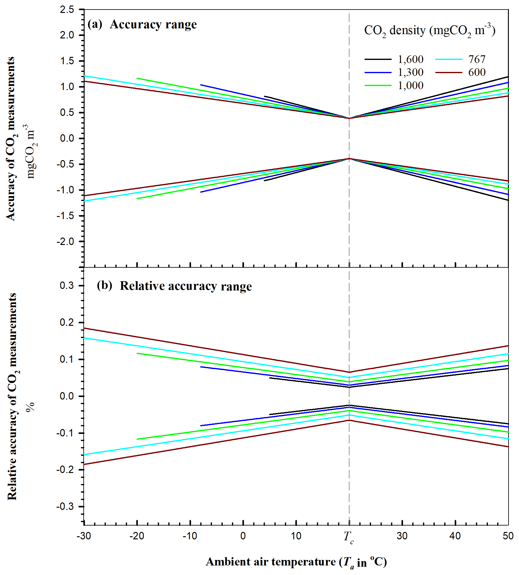
Figure 2Accuracy of field CO2 measurements from open-path eddy-covariance flux systems by EC150 infrared CO2–H2O analyzers (Campbell Scientific Inc., UT, USA) over their operational range in Ta at atmospheric pressure of 101.325 kPa. The vertical dashed line represents ambient air temperature Tc at which an analyzer was calibrated, zeroed, and/or spanned. Above 5 ∘C, accuracy is evaluated up to the possible maximum CO2 density in ecosystems (black curves). Assume that this maximum CO2 density starts linearly decreasing at 5 ∘C to the atmospheric CO2 background value 767 mgCO2 m−3 at −30 ∘C. Accordingly, below 5 ∘C, the accuracy for CO2 density at a level above the background value (green, blue, or black curves) is evaluated up to this decreasing trend of CO2 densities. Relative accuracy of CO2 measurements is the ratio of CO2 accuracy to CO2 density.
Table 2Accuracies of field CO2 and H2O measurements from open-path eddy-covariance systems by EC150 infrared CO2–H2O analyzers (Campbell Scientific Inc., UT, USA) on the major background values of ambient air temperature, CO2, and H2O in ecosystems. (Atmospheric pressure: 101.325 kPa. Calibration ambient air temperature: 20 ∘C.)
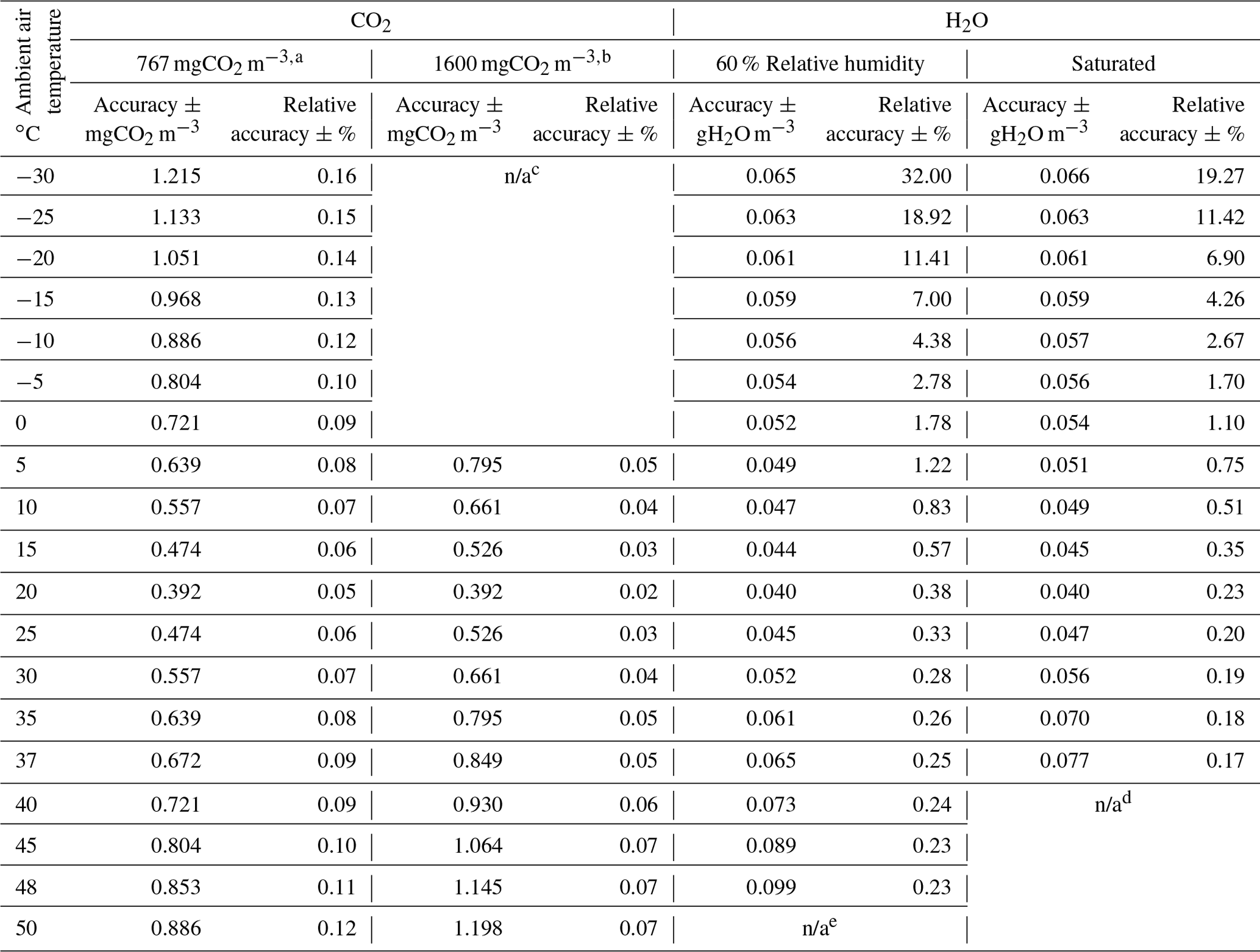
a 767 mgCO2 m−3 is the atmospheric background CO2 density (Global Monitoring Laboratory, 2022). b 1600 mgCO2 m−3 is assumed to be the maximum CO2 density in ecosystems. c CO2 density in ecosystems is assumed to be lower than 1600 mgCO2 m−3 when ambient air temperature is below 5 ∘C. d H2O density in saturated air above 37 ∘C is out of the measurement range of EC150 infrared CO2–H2O analyzers (0–44 gH2O m−3). e H2O density in air of 60 % relative humidity above 48 ∘C is out of the measurement range of EC150 infrared CO2–H2O analyzers (0–44 gH2O m−3). n/a denotes “not applicable”.
Model (2) defines the accuracy of field H2O measurements from OPEC systems by infrared analyzers () as
where is H2O zero drift uncertainty, is H2O gain drift uncertainty, is cross-sensitivity-to-CO2 uncertainty, and is H2O precision uncertainty. Using the same approach as for , is formulated as
where , as defined in Table 1, is the precision of the infrared analyzers for H2O measurements. The other uncertainty terms in Model (15) can be understood and formulated using a similar approach for their counterparts in Model (3).
5.1 (H2O zero drift uncertainty) and (H2O gain drift uncertainty)
The model of the analyzer working equation for is similar to Model (5) for in formulation, given also by the derivations in the “Theory and operation” section in LI-COR Biosciences (2001, 2021b, c):
where awi (i=1, 2, or 3) is a coefficient of the 3-order polynomial in the terms inside curly brackets; Sc is the cross-sensitivity of a detector to CO2, while detecting H2O, at the wavelength for H2O measurements (hereafter referred to as sensitivity to CO2); Zw is the H2O zero adjustment (i.e., H2O zero coefficient); Gw is the H2O gain adjustment (i.e., commonly referred as to H2O span coefficient); and Aw, Aws, Ac, and Acs represent the same things as in Model (5). The parameters of awi, Zw, Gw, and Sc in Model (17) are statistically estimated to establish an H2O working equation in the production calibration against a series of air standards with different H2O contents under ranges of and P (i.e., calibration). The H2O working equation (i.e., Model 17 with estimated parameters) is used inside the analyzer OS to compute as the closest proxy for true from field measurements of Aw, Aws, Ac, Acs, and P.
Because of the similarities in model principles and parameter implications between Models (5) and (17), following the same analyses and rationales as for and , is formulated as
and is formulated as
5.2 (sensitivity-to-CO2 uncertainty)
The infrared light at wavelength of 2.7 µm for H2O measurement is traceably absorbed by CO2 (see Fig. 4.7 in Wallace and Hobbs, 2006). This absorption interferes slightly with the H2O absorption at this wavelength (McDermitt et al., 1993). As such, the power of identical measurement lights (i.e., Aws as a steady value in the H2O working equation from Model 17) through several air standards with the same H2O density but different backgrounds of CO2 amounts would result in different values of Aw in the H2O working equation from Model (17). In this equation, without parameter Sc and its joined term, different Aw values will result in significantly different values, although is essentially the same. In case of the same H2O amount in the airflows under different CO2 backgrounds, different values of Aw reporting the same are accounted for by Sc associated with Ac and Acs in the H2O working equation from Model (17). However, Sc is not perfectly accurate either, having uncertainty in the determination of . This uncertainty in the EC150 infrared analyzer is specified by the sensitivity to CO2 () as the maximum range of gH2O m−3 (mgCO2 m−3)−1 (Table 1). Assuming the infrared analyzers for H2O have the lowest sensitivity-to-CO2 uncertainty for airflow with an atmospheric background CO2 amount (i.e., 767 mgCO2 m−3), could be formulated as
Accordingly, can be reasonably expressed as
5.3 (H2O measurement accuracy)
Substituting Eqs. (16), (18), (19), and (21) into Model (15), for an individual H2O measurement from OPEC systems by infrared analyzers can be expressed as
This equation is the H2O accuracy equation for the OPEC systems with infrared analyzers. It expresses the accuracy of H2O measurements from the OPEC systems in terms of the analyzer specifications , , dwz, , Trh, and Trl; measured variables and Ta; and a known variable Tc. Using this equation and the specification values as in Table 1 for EC150 infrared analyzers, the accuracy of field H2O measurements can be evaluated as a range for OPEC systems with such analyzers. For an OPEC system with another model of open-path infrared analyzer, such as the LI-7500 series (LI-COR Biosciences, NE, USA) or IRGASON (Campbell Scientific Inc., UT, USA), its corresponding specification values are used.
5.4 Evaluation of
H2O accuracy () can be evaluated using the H2O accuracy equation over a domain of Ta and . Similar to the CO2 accuracy equation in Fig. 2, is presented as the ordinate along the abscissa of Ta at different levels within the ranges of Ta and in ecosystems (Fig. 3). As with the evaluation of , Ta is limited from −30 to 50 ∘C and Tc can be assumed to be 20 ∘C. The range of at Ta needs to be determined using atmospheric physics (Buck, 1981).
5.4.1 range
The EC150 analyzers were calibrated for H2O density from 0 to 44 gH2O m−3 due to the reason addressed in Sect. 2. The highest limit of measurement range for H2O density by other models of analyzers also should be near 44 gH2O m−3. However, due to the positive exponential dependence of air water vapor saturation on Ta (Wallace and Hobbs, 2006), has a range that is wider at higher Ta and narrower at lower Ta. Below 37 ∘C at 101.325 kPa, is lower than 44 gH2O m−3, and its range becomes narrower and narrower, reaching 0.34 gH2O m−3 at −30 ∘C. To determine the H2O accuracy over the same relative range of air moisture, even at different Ta, the saturation water vapor density is used to scale air moisture to 20 %, 40 %, 60 %, 80 %, and 100 % (i.e., relative humidity or RH). For each scaled RH value, can be calculated at different Ta and P (Appendix B) for use in the H2O accuracy equation. In this way, over the range of Ta, H2O accuracy can be shown as curves, along each of which RH is equal (Fig. 3).
5.4.2 range
In the same way as with CO2 accuracy, the H2O accuracy at Ta=Tc is best at its narrowest as the sum of precision and sensitivity-to-CO2 uncertainties (<0.040 gH2O m−3 in magnitude). However, away from Tc, its range non-linearly becomes wider, very gradually below this Tc value but more abruptly above because, as Ta increases, at the same RH increases exponentially (Eqs. B1 and B2 in Appendix B), while increases linearly with in the H2O accuracy Eq. (22). This range can be summarized as the widest at 48 ∘C as ±0.099 gH2O m−3 for air with 60 % RH (Fig. 3a and H2O columns in Table 2). The number can be rounded up to ±0.10 gH2O m−3 for the overall accuracy of field H2O measurements from OPEC systems by the EC150 infrared analyzers.
Figure 3b shows an interesting trend of H2O relative accuracy with Ta. Given the RH range, as shown in Fig. 3b, the relative accuracy diverges with a Ta decrease and converges with a Ta increase. The H2O relative accuracy varies from 0.17 % for saturated air at 37 ∘C to 96 % for 20 % RH air at −30 ∘C (data for Fig. 3b) and, at this low Ta, can be much greater if RH goes further lower. The H2O relative accuracy in magnitude is <1 % while gH2O m−3, <5 % while gH2O m−3, and >10 % while gH2O m−3.
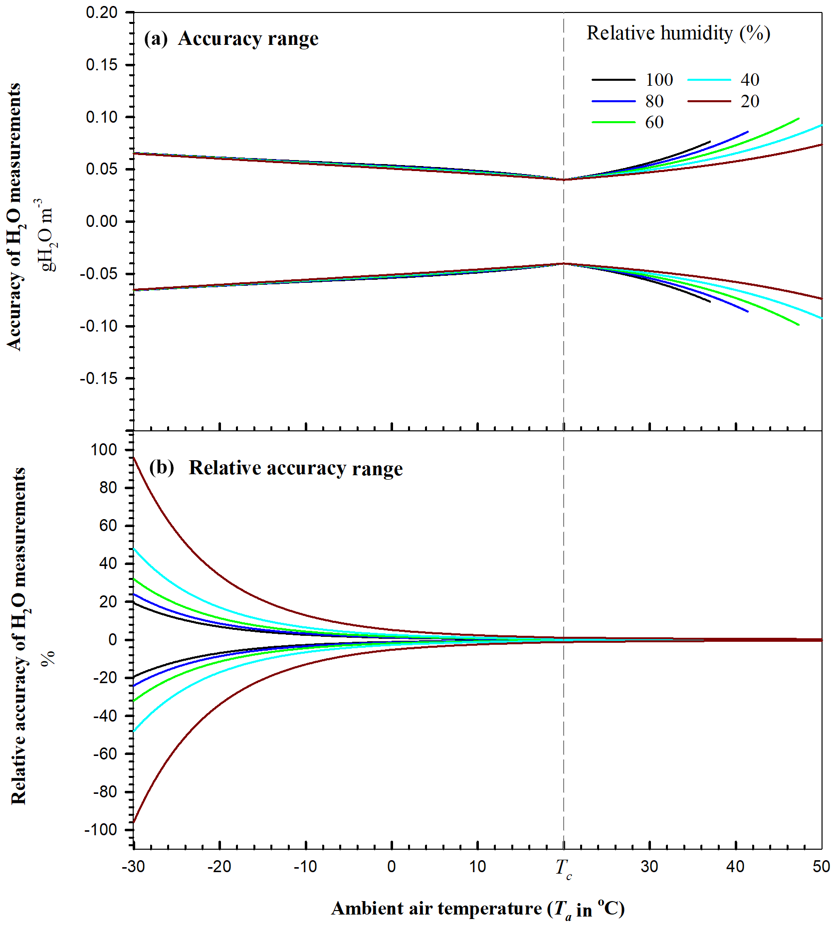
Figure 3Accuracy of field H2O measurements from open-path eddy-covariance systems by EC150 infrared CO2–H2O analyzers (Campbell Scientific Inc., UT, USA) over their operational range in Ta under atmospheric pressure of 101.325 kPa. The vertical dashed line represents the ambient air temperature (Tc) at which an analyzer was calibrated, zeroed, and/or spanned. Relative accuracy of H2O measurements is the ratio of H2O accuracy to H2O density.
The primary objective of this study is to develop an assessment methodology to evaluate the overall accuracies of field CO2 and H2O measurements from the infrared analyzers in OPEC systems by compositing their individual measurement uncertainties as specified with four uncertainty descriptors: zero drift, gain drift, sensitivity to , and precision variability (Table 1). Ultimately, the overall accuracies (i.e., and ) make uncertainty analyses possible for the various applications of CO2 and H2O data, and the composited accuracy equations (i.e., Eqs. 14 and 22) make the field maintenance rationale for infrared analyzers.
6.1 Application of and to the uncertainty analyses for CO2 and H2O flux data
As discussed in Introduction, the uncertainty in each flux data point is contributed by numerous sub-uncertainties in the processes of measurements and computations, among which and are two fundamental uncertainties in the measurements from infrared analyzers. For this study topic, assuming 3-D wind speeds are accurately measured by a sonic anemometer, Appendix C demonstrates that neither nor brings an uncertainty into the covariance of vertical wind speed (w) with , , or Ta even after coordinate rotations, lag maximization, and low- and high-frequency corrections, given by Eqs. (C8) and (C9) in Appendix C as
where the overbar is a Reynolds' averaging operator, prime denotes the fluctuations in a variable away from its mean (e.g., ), subscript T indicates “true” value (see Appendix C for the implication of true value), and subscript rmf indicates that the covariance was corrected through coordinate rotations (r), lag maximization (m), and low- and high-frequency corrections (f). The three equalities in Eq. (23) that are proved in Appendix C prove that the measured covariance of w with , , or Ta is not affected by corresponding , , or ΔTa (i.e., accuracy of Ta), being equal to the true covariance. Further, through WPL corrections, the three terms on the left side of Eq. (23) can be used to derive an analytical equation for measured CO2 or H2O flux, whereas the three terms on the right side of this equation can be used to derive an analytical equation for true CO2 or H2O flux. The comparison of both analytical equations can demonstrate the partial effects of and on the uncertainty in CO2 or H2O flux data.
6.1.1 Roles of and in the uncertainty in CO2 flux data
Using the terms on the left side of Eq. (23), through the WPL corrections for CO2 flux from (Webb et al., 1980), the measured CO2 flux () is given by
where μ is the ratio of dry air to water molecular weight, ρd is dry air density, and TaK is air temperature in kelvin. According to Eqs. (C1) and (23), this equation can be written as
where is the accuracy of . is well defined as ±0.20 K in compliance with the WMO standard (WMO, 2018). According to Eqs. (23) and (24), from , the nominal true CO2 flux () can be given by
From Eqs. (25) and (26), the uncertainty in CO2 flux () can be expressed as
This derivation provides a conceptual model for the partial effects of and on the uncertainty in CO2 flux data. This uncertainty is added by and interactively with the density effect due to H2O flux (i.e., the term with in Eq. 27) and temperature flux (i.e., the term with in Eq. 27).
6.1.2 on uncertainty in H2O flux data
Using the same approach to Eq. (27), the uncertainty in H2O flux () can be expressed as
This formulation provides a conceptual model for the partial effects of on the uncertainty in H2O flux data. This uncertainty is added only by also interactively with the density effect due to H2O flux (i.e., the term with in Eq. 28) and temperature flux (the term with in Eq. 28). Further analysis and more discussion about Eqs. (27) and (28) go beyond the scope of this study.
6.2 Application of to the uncertainty analysis for high-frequency air temperature
The measured variables , along with Ts and P, can be used to compute high-frequency Ta in OPEC systems (Swiatek, 2018). If were an exact function from the theoretical principles, it would not have any error itself. However, in our applications, variables , Ts, and P are measured from the OPEC systems experiencing seasonal climates. As addressed in this study, the measured values of these variables have measurement uncertainty in (, i.e., accuracy of field H2O measurement), in Ts (ΔTs, i.e., accuracy of field Ts measurement), and in P (ΔP, i.e., accuracy of field P measurement). The uncertainties from the measurements propagate to the computed Ta as an uncertainty (ΔTa, i.e., accuracy of ). This accuracy is a reference by any application of Ta. It should be specified through the relationship of ΔTa to , ΔTs, and ΔP.
As field measurement uncertainties, , ΔTs, or ΔP are reasonably small increments in numerical analysis (Burden et al., 2016). As such, depending on all the small increments, ΔTa is a total differential of with respect to , Ts, and P, which are measured independently by three sensors, given by
In this equation, from the application of Eq. (22) is a necessary term to acquire ΔTa, ΔTs can be acquired from the specifications for 3-D sonic anemometers (Zhou et al., 2018), ΔP can be acquired from the specifications for the barometer used in the OPEC systems (Vaisala, 2020), and the three partial derivatives can be derived from the explicit function . With , ΔTs, ΔP, and the three partial derivatives,ΔTa can be ranged as a function of , Ts, and P.
6.3 Application of accuracy equations in analyzer field maintenance
An infrared analyzer performs better if the field environment is near its manufacturing conditions (e.g., Ta at 20 ∘C), which is demonstrated in Figs. 2a and 3a for measurement accuracies associated with Tc. As indicated by the accuracies in both figures, the closer to Tc at 20 ∘C Ta is, the better the analyzers perform. However, the analyzers are used in OPEC systems mostly for long-term field campaigns through four-seasonal climates vastly different from those in the manufacturing processes. Over time, an analyzer gradually drifts in some ways and needs field maintenance, although within its specifications.
The field maintenance cannot improve the sensitivity-to- uncertainty and precision variability, but both are minor (their sum <0.392 mgCO2 m−3 for CO2, Eqs. 4 and 13; <0.045 gH2O m−3 for H2O, Eqs. 16 and 21) as compared to the zero or gain drift uncertainties. However, the zero and gain drift uncertainties are major in the determination of field measurement accuracy (Figs. 2 to 4 and Eqs. 14 and 22), but they are adjustable, through the zero and/or span procedures, and can be minimized. Therefore, manufacturers of infrared analyzers have provided software and hardware tools for the procedures (Campbell Scientific Inc., 2021b) and scheduled the procedures using those tools (LI-COR Biosciences, 2021c). Fratini et al. (2014) provided a technique implemented into the EddyPro® Eddy Covariance Software (LI-COR Biosciences, 2021a) to correct the drift biases from a raw time series of CO2 and H2O data through post-processing. This study provides rationales for how to assess, schedule, and perform the zero and span procedures (Figs. 2a, 3a, and 4).
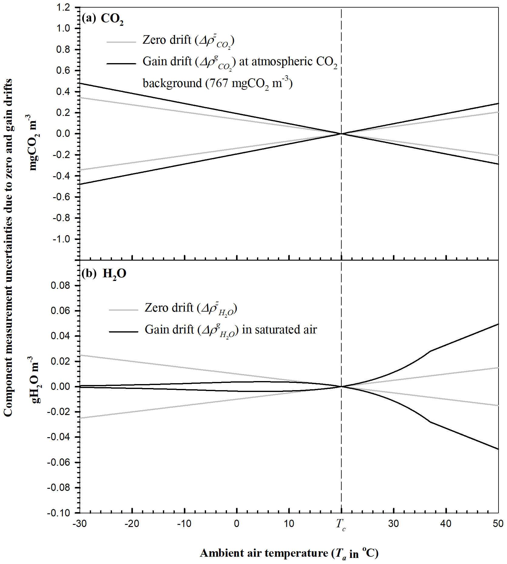
Figure 4Component measurement uncertainties due to the zero and gain drifts of EC150 infrared CO2–H2O analyzers (Campbell Scientific Inc, UT, USA) in open-path eddy-covariance flux systems over their operational range in Ta under an atmospheric pressure of 101.325 kPa. The vertical dashed line represents the ambient air temperature (Tc) at which an analyzer was calibrated, zeroed, and/or spanned.
6.3.1 CO2 zero and span procedures
Figure 4a shows that the CO2 zero drift uncertainty linearly increases with Ta away from Tc over the full Ta range within which OPEC systems operate; so, too, does CO2 gain drift uncertainty increase for a given CO2 concentration. As suggested by Zhou et al. (2021), both drifts should be adjusted near the Ta value around which the system runs. The zero and gain drifts should be adjusted, through zero and span procedures, at a Ta close to its daily mean around which the system runs. Based on the range of Ta daily cycle, the procedures are set at a moderate instead of the highest or lowest moment in Ta. Given the daily cycle range is much narrower than 40 ∘C, an OPEC system could run at Ta within ±20 of Tc if the procedures are performed at a right moment of Ta. For our case study on atmospheric CO2 background (left CO2 column in Table 2), the procedures can narrow the widest possible range of ±1.22 mgCO2 m−3 for field CO2 measurement by at least 40 % to ±0.72 mgCO2 m−3 (i.e., accuracy at 0 or 40 ∘C when Tc=20 ∘C), which would be a significant improvement to ensure field CO2 measurement accuracy through CO2 zero and span procedures.
6.3.2 H2O zero and span procedures
Figure 4b shows that the H2O zero drift uncertainty increases as Ta moves away from Tc in the same trend as CO2 zero drift uncertainty. Therefore, an H2O zero procedure can be performed by the same technique as for the CO2 zero procedure. H2O gain drift uncertainty has a different trend. It exponentially diverges, as Ta increases away from Tc, to gH2O m−3 near 50 ∘C and gradually converges to 2 orders smaller as Ta decreases away from Tc, to gH2O m−3 at −30 ∘C (data for Fig. 4b). The exponential divergence results from the linear relationship of H2O gain drift uncertainty (Eq. 19) with , which exponentially increases (Eq. B1) with a Ta increase away from Tc for the same RH (Buck, 1981). The convergence results from the linear relationship offset by the exponential decrease in with a Ta decrease for the same RH. This trend of H2O gain drift uncertainty with Ta is a rationale to guide the H2O span procedure, which adjusts the H2O gain drift.
The H2O span procedure needs standard moist air with known H2O density from a dew point generator. The generator is not operational near or below freezing conditions (LI-COR Biosciences, 2004), which limits the span procedure to be performed only under non-freezing conditions. This condition, from 5 to 35 ∘C, may be considered for the generator to be conveniently operational in the field. Accordingly, the zero and span procedures for H2O should be discussed separately for a Ta above and below 5 ∘C.
Ta above 5 ∘C
Looking at the right portion with Ta above 5 ∘C in Fig. 4b, H2O gain drift has a more obvious impact on measurement uncertainty in a higher Ta range (e.g., above Tc), within which the H2O span procedure is most needed. In this range, the maximum accuracy range of ±0.10 gH2O m−3 can be narrowed by 30 % to ±0.07 (assessed from data for Fig. 3a) if the zero and span procedures for H2O can be sequentially performed as necessary in a Ta range from 5 to 35 ∘C.
Ta below 5 ∘C
Looking at the left portion with Ta below 5 ∘C in Fig. 4b, H2O gain drift has a less obvious contribution to the measurement uncertainty in a lower Ta range (e.g., below 5 ∘C), within which the H2O span procedure may be unnecessary. An H2O gain drift uncertainty at 5 ∘C is 50 % of the H2O zero drift uncertainty (dotted curve in Fig. 5). This percentage decreases to 3 % at −30 ∘C. On average, this percentage over a range of −30 to 5 ∘C is 18 % (assessed from data for the dotted curve in Fig. 5). Thus, for H2O measurements over the lower Ta range, it can be concluded that H2O zero drift is a major uncertainty source, and H2O gain drift is a minor uncertainty source.
A close examination of the other curves in Fig. 5 for the portion in the accuracy range from H2O zero/gain drift makes this conclusion more convincing. Given Tc=20, in the accuracy range, the portion from H2O zero drift uncertainty is much greater (maximum 38 % at −30 ∘C) than that from H2O gain drift uncertainty (maximum only 7 % at 5 ∘C). On average over the lower Ta range, the former is 27 % and the latter only 4 %. Further, given Tc=5 ∘C, in the accuracy range, the portion from H2O gain drift uncertainty is even smaller (maximum only 3 % at −5 ∘C); in contrast, the portion from zero drift uncertainty is more major (1 order higher, 30 % at −30 ∘C). On average over the lower Ta range, the minor gain drift uncertainty is 1.7 %, and the major zero drift uncertainty is 17 %. Both percentages underscore that the H2O span procedure is reasonably unnecessary under cold/dry conditions, and, under such conditions, the H2O zero procedure is the only necessary option to efficiently minimize H2O measurement uncertainty from the infrared analyzers in OPEC systems. This finding gives confidence in H2O measurement accuracy to users who are worried about H2O span procedures for infrared analyzers in the cold seasons when a dew point generator is not operational in the field (LI-COR Biosciences, 2004).
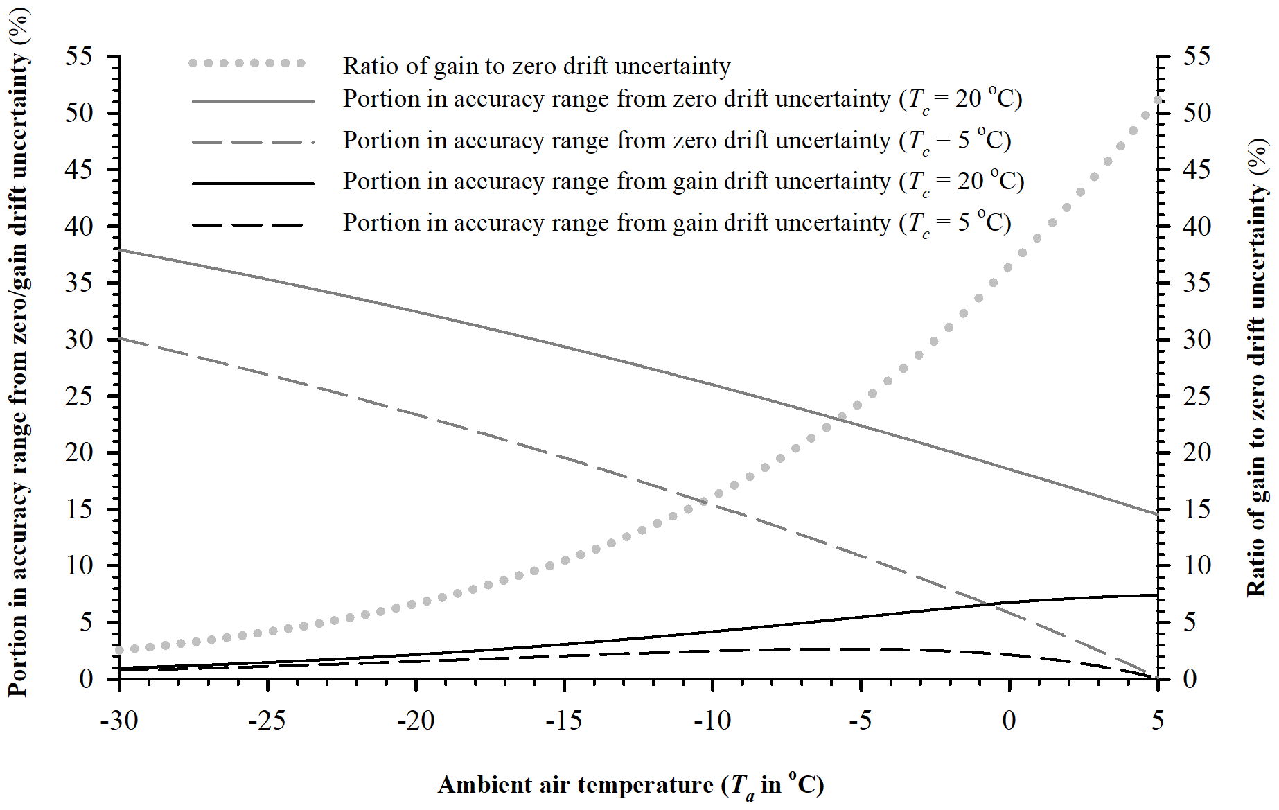
Figure 5For a range of low Ta, the portion in the accuracy range from zero/gain drift uncertainty (left ordinate) and the ratio of gain to zero drift uncertainty (right ordinate). The curves are evaluated by Eqs. (18), (19), and (22) from measurement specifications for EC150 infrared CO2–H2O analyzers (Campbell Scientific Inc, UT, USA) in open-path eddy-covariance flux systems over the Ta range from −30 to 5 ∘C under atmospheric pressure of 101.325 kPa. Tc is the ambient air temperature at which an analyzer was calibrated, zeroed, and/or spanned.
6.3.3 H2O zero procedure in cold and/or dry environments
In cold environments, although the non-operational H2O span procedure is unnecessary, the H2O zero procedure is asserted to be a prominently important option for minimizing the H2O measurement uncertainty from the infrared analyzers in OPEC systems. This procedure, although operational under freezing conditions, is still inconvenient for users when the weather is very cold (e.g., when Ta is below −15 ∘C). If the field H2O zero procedure is performed as needed above this Ta value, while an OPEC system runs at Ta within ±20 ∘C of Tc, the poorest H2O accuracy of ±0.066 gH2O m−3 below 5 ∘C in Table 2 can be narrowed, through the H2O zero procedure, by at least 22 % to 0.051 gH2O m−3 (assessed from data for Fig. 3a). Correspondingly, the relative accuracy range can be narrowed by the same percentage. The H2O zero procedure can ensure both accuracy and relative accuracy of H2O measurements in a cold environment (Fratini et al., 2014). In a dry environment, it plays the same role as in a cold environment, but it would be more convenient for users to perform the zero procedure if warmer.
In a cold and/or dry environment, H2O zero procedures on a regular schedule would best minimize the impact of zero drifts on measurements. Under such an environment, the automatic zero procedure for CO2 and H2O together in CPEC systems is an operational and efficient option to ensure and improve field CO2 and H2O measurement accuracies (Campbell Scientific Inc., 2021a; Zhou et al., 2021).
An assessment methodology to evaluate the overall accuracies of field CO2 and H2O measurements from the infrared analyzers in OPEC systems is developed using individual analyzer measurement uncertainties as specified using four uncertainty descriptors: zero drift, gain drift, sensitivity to , and precision variability (Table 1). For the evaluation, these uncertainty descriptors are comprehensively composited into the accuracy Model (2) and then formulated as a CO2 accuracy Eq. (14) and an H2O accuracy Eq. (22) (Sects. 3 to 5 and Appendix A). The assessment methodology, along with the model and the equations, presents our development for the objective (Sects. 4.5 and 5.4).
7.1 Accuracy model
Accuracy Model (2) composites the four measurement uncertainties (zero drift, gain drift, sensitivity to , and precision variability), specified for analyzer performance, as an accuracy range. This range is modeled as a simple addition of the four uncertainties. The simple addition is derived from our analysis assertion that the four measurement uncertainties interactionally or independently contribute to the accuracy range, but the contributions from the interactions inside any pair of uncertainties are negligible since they are 3 orders smaller in magnitude than an individual contribution in the pair (Appendix A). This derived model is simple and applicable, paving an approach to the formulation of accuracy equations that are computable for evaluating the overall accuracies of field CO2 and H2O measurements from the infrared analyzers in OPEC systems.
Additionally, included in the accuracy model, the four types of measurement uncertainty sources (i.e., zero drift, gain drift, sensitivity to , and precision variability) to specify the performance of infrared CO2–H2O analyzers for OPEC systems have been consistently used over last 2 decades (LI-COR Biosciences, 2001, 2021b, c; Campbell Scientific Inc., 2021a, b). With the advancement of optical technologies, the number of these uncertainty sources for analyzer specifications is not expected to increase; rather some current uncertainty sources could be eliminated from the current specification list, even if not in the near future. If eliminated, in Models (3) and (15) and Eqs. (14) and (22), the parameters and variables related to the eliminated uncertainty sources could be easily removed for the adoption of the new set of specifications for infrared CO2–H2O analyzers.
7.2 Formulation of uncertainty terms in Model (2) for accuracy equations
In Sects. 4 and 5, each of the four uncertainty terms in accuracy Model (2) is formulated as a computable sub-equation for CO2 (Eqs. 4, 7, 11, and 13) and H2O (Eqs. 16, 18, 19, and 21), respectively. The accuracy model, whose terms are replaced with the formulated sub-equations for CO2, becomes a CO2 accuracy Eq. (14) and, for H2O, becomes an H2O accuracy Eq. (22). In the formulation, approximation is used for zero drift, gain drift, and sensitivity to , while statistics are applied for precision variability.
For the zero/gain drift, although it is well known that the drift is influenced more by Ta if housing CO2–H2O accumulation is assumed to be minimized as insignificant under normal field maintenance (LI-COR Biosciences, 2021c; Campbell Scientific Inc., 2021b), the exact relationship of drift to Ta does not exist. Alternatively, the zero/gain drift uncertainty is formulated by an approximation of drifts away from Tc linearly in proportion to the difference between Ta and Tc but within its maximum range over the operational range in Ta of OPEC systems (Eqs. 7, 11, 18, and 19). A drift uncertainty equation formulated through such an approximation is not an exact relationship of drift to Ta, but it does represent the drift trend, as influenced by Ta, to be understood by users. The accuracy from this equation at a given Ta is not exact either, but the maximum range over the full range, which is the greatest-likelihood estimation, is most needed by users.
In fact, the H2O accuracy as influenced by the linear trend of zero and gain drifts with the difference between Ta and Tc is overshadowed by the exponential trend of saturated H2O density with Ta (Fig. 4b). Similarly, the CO2 accuracy as influenced by the linear trend of zero and gain drifts with this difference is dominated by the CO2 density of the ecosystem background with Ta, particularly in the low temperature range (Fig. 2). Ultimately, the assumed linear trend does not play a dominant role in the accuracy trends of CO2 and H2O, which shows the merits of our methodology in the uses of atmospheric physics and biological environment principles for the field data.
The sensitivity-to- uncertainty can be formally formulated as Eqs. (20) or (12), but, if directly used, this formulation would add an additional variable to the accuracy equation. Equation (12) would add H2O density () to the CO2 accuracy Eq. (14), and Eq. (20) would add CO2 density () to the H2O accuracy Eq. (22). For either accuracy equation, the additional variable would complicate the uncertainty analysis. According to the ecosystem environment background, the maximum range of sensitivity-to- uncertainty is known, and as compared to the major uncertainty in zero/gain drift (Table 1), this range is narrow (Table 1 and Eqs. 13 and 21). Therefore, the sensitivity-to- uncertainty is approximated as Eq. (21) or (13). This approximation widens the accuracy range slightly, in a magnitude smaller than each of major uncertainties from the drifts by at least 1 order; however, it eliminates the need for in the CO2 accuracy Eq. (14) and for in the H2O accuracy Eq. (22), which makes the equations easily applicable.
Precision uncertainty is statistically formulated as Eq. (4) for CO2 and Eq. (16) for H2O. This formulation is common practice based on statistical methods (Hoel, 1984).
7.3 Use of relative accuracy for infrared analyzer specifications
Relative accuracy is often used concurrently with accuracy to specify sensor measurement performance. The accuracy is the numerator of relative accuracy whose denominator is the true value of a measured variable. When evaluated for the applications of OPEC systems in ecosystems, CO2 accuracy in magnitude is small in a range within 1 order (0.39–1.22 mgCO2 m−3, data for Fig. 2a), and so is H2O accuracy (0.04–0.10 gH2O m−3, data for Fig. 3a). In ecosystems, CO2 is naturally high, as compared to its accuracy magnitude, and does not change much in terms of a magnitude order (e.g., no more than 1 order from 600 to 1600 mgCO2 m−3, assumed in this study). However, unlike CO2, H2O naturally changes dramatically in its amount across at least 3 orders in magnitude (e.g., at 101.325 kPa, from 0.03 gH2O m−3 when RH is 10 % at −30 ∘C to 40 gH2O m−3 when dew point temperature is 35 ∘C at the highest as reported by the National Weather Service, 2022; under drier conditions, the H2O amount could be even lower). Because, in ecosystems, CO2 changes differently from H2O in amount across magnitude orders, the relative accuracy behaviors in CO2 differ from H2O (Figs. 2b and 3b).
7.3.1 CO2 relative accuracy
Because of the small CO2 accuracy magnitude relative to the natural CO2 amount in ecosystems, the CO2 relative accuracy magnitude varies within a narrow range of ±0.07 to ±0.19 % (Sect. 4.5.2). If the relative accuracy is used, either a range of ±0.07 to ±0.19 % or an inequality of ≤ 0.19 % in magnitude can be specified as the CO2 relative accuracy for field CO2 measurements. Both range and inequality would be equivalently perceived by users to be a fair performance of the infrared analyzers in OPEC systems. For simplicity, our study specifies the CO2 relative accuracy for the EC150 infrared analyzers to be ±0.19 % after a manufacturing calibration (data shown in Fig. 2b).
7.3.2 H2O relative accuracy
Although the H2O accuracy magnitude is also small, the “relatively” great change in natural-air H2O across several magnitude orders in ecosystems results in a much wider range of the H2O relative accuracy magnitude, from ±0.23 % at maximum air moisture to ±96 % when RH is 20 % at −30 ∘C (Fig. 3b and Sect. 5.4.2). H2O relative accuracy can be much greater under dry conditions at low Ta (e.g., ±192 % for air when RH is 10 % at −30 ∘C). Accordingly, if the relative accuracy is used, either a range of ±0.23 % to ±192 % or an inequality of ≤ 192 % in magnitude can be specified as the H2O relative accuracy for field H2O measurements. Either the range or the inequality could be perceived by users intrinsically as a poor measurement performance of the infrared analyzers in OPEC systems, although either specification is conditionally right for fair H2O measurement.
Apparently, the relative accuracy for H2O measurements in ecosystems is not intrinsically interpretable by users to correctly perceive the performance of the infrared analyzers in OPEC systems. Instead, if H2O relative accuracy is unconditionally specified just in an inequality of ≤ 192 % in magnitude, it could easily mislead users to wrongly assess the performance as unacceptable for H2O measurements, although this performance of the infrared analyzers in OPEC systems is fair for air when RH is 10 % at −30 ∘C. Therefore, H2O relative accuracy is not recommended to be used for specification of infrared analyzers for H2O measurement performance. If this descriptor is used, the H2O relative accuracy under a standard condition should be specified. This condition may be defined as saturated air at 35 ∘C (i.e., the highest natural dew point; National Weather Service, 2022) under normal P of 101.325 kPa (Wright et al., 2003). For our case study, under such a standard condition, the H2O relative accuracy can be specified within ±0.18 % after a manufacturing calibration (data for Fig. 3b).
The accuracy of field measurements from the infrared analyzers in OPEC systems can be defined as a maximum range of composited measurement uncertainty (Eqs. 14 and 22) from the specified sources: zero drift, gain drift, sensitivity to , and precision variability (Table 1), all of which are included in the system specifications for infrared CO2–H2O analyzers currently used in field OPEC systems. The specified uncertainties interactionally or independently contribute to the overall uncertainty. Fortunately, the interactions between component uncertainties in each pair is 3 orders smaller than either component individually (Appendix A). Therefore, these specified uncertainties can be simply added together as the accuracy range in a general accuracy model for the infrared analyzers in OPEC systems (Model 2). Based on statistics, bio-environment, and approximation, the specification descriptors of the infrared analyzers in OPEC systems are incorporated into the model terms to formulate the CO2 accuracy Eq. (14) and the H2O accuracy Eq. (22), both of which are computable to evaluate corresponding CO2 and H2O accuracies. For the EC150 infrared analyzers used in the OPEC systems over their operational range in Ta at the standard P of 101.325 kPa (Figs. 2 and 3 and Table 2), the CO2 accuracy can be specified as ±1.22 mgCO2 m−3 (relatively within ±0.19 %, Fig. 2) and H2O accuracy as ±0.10 gH2O m−3 (relatively within ±0.18 % for saturated air at 35 ∘C at the standard P, Fig. 3).
Both accuracy equations are not only applicable for further uncertainty estimation for CO2 and H2O fluxes due to CO2 and H2O measurement uncertainties (Eqs. 27 and 28) and the error/uncertainty analyses in CO2 and H2O data applications (e.g., Eq. 29); they may also be used as a rationale to assess and guide field maintenance on infrared analyzers. Equation (14) as shown in Fig. 2a, along with Eqs. (7) and (11) as shown in Fig. 4a, guides users to adjust the CO2 zero and CO2 gain drifts, through the corresponding zero and span procedures, near a Ta value that minimizes the Ta departures, on average, during the period of interest if this period were not under extreme and hazard conditions (Fratini et al., 2014). As assessed on atmospheric CO2 background, the procedures can narrow the maximum CO2 accuracy range by 40 %, from ±1.22 to ±0.72 mgCO2 m−3 and thereby greatly improve the CO2 measurement accuracies with these regular zero and span procedures for CO2.
Equation (22) as shown in Fig. 3a, along with Eqs. (18) and (19) as shown in Fig. 4b, presents users with a rationale to adjust the H2O zero drift of infrared analyzers in the same technique as for CO2, but the H2O gain drift under hot and humid environments needs more attention (see the right portion above Tc in Figs. 3a and 4b); under cold and/or dry environments, it does not merit further concern (see the left portion below 0 ∘C in Fig. 4b). In a Ta range above 5 ∘C, the maximum H2O accuracy range of ±0.10 gH2O m−3 can be narrowed by 30 % to ±0.07 gH2O m−3 if both zero and span procedures for H2O are performed as necessary. In a Ta range below 5 ∘C, the H2O zero procedure alone can narrow the maximum H2O accuracy range of ±0.066 gH2O m−3 by 22 % to ±0.051 gH2O m−3. Under cold environmental conditions, the H2O span procedure is found to be unnecessary (Fig. 5), and the H2O zero procedure is proposed as the only, and prominently efficient, option to minimize H2O measurement uncertainty from the infrared analyzers in OPEC systems. This procedure plays the same role under dry conditions. Under cold and/or dry environments, the zero procedure for CO2 and H2O together would be a practical and efficient option not only to warrant but also to improve measurement accuracy. In a cold environment, adjusting the H2O gain drift is impractical because of the failure of a dew point generator under freezing conditions.
Additionally, as a specification descriptor for OPEC systems used in ecosystems, relative accuracy is applicable for CO2 instead of H2O measurements. A small range in the CO2 relative accuracy can be perceived intuitively by users as normal. In contrast, without specifying the condition of air moisture, a large range in H2O relative accuracy under cold and/or dry conditions (e.g., 100 %) can easily mislead users to an incorrect conclusion in interpretation of H2O measurement reliability, although it is the best achievement of the modern infrared analyzers under such conditions. If the H2O relative accuracy is used, the authors suggest conditionally defining it for saturated air at 35 ∘C (i.e., 39.66 gH2O m−3 at 101.352 kPa). Ultimately, this study provides some scientific bases for the flux community to specify the accuracy of CO2–H2O measurements from the infrared analyzers in OPEC systems, although only one model of infrared analyzers (i.e., EC150) is used for this study.
As defined in the Introduction, the measurement accuracy of infrared CO2–H2O analyzers is a range of the difference between the true α density (ραT, where α can be either CO2 or H2O) and α density (ρα) measured by the analyzers. The difference is denoted by Δρα, given by Eq. (1) in Sect. 3. The range of this difference is contributed from the analyzer performance uncertainties, as specified by the use of the four descriptors: zero drift, gain drift, cross-sensitivity, and precision (LI-COR Biosciences, 2021c; Campbell Scientific Inc., 2021b).
According to the definitions in Sect. 2, zero drift uncertainty () is independent of ραT value and gain trend related to analyzer response; so, too, is cross-sensitivity uncertainty (), which depends upon the amount of background H2O in the measured air if α is CO2 and upon the amount of background CO2 in the measured air if α is H2O. In the case that both gain drift and precision uncertainties are zero, and are simply additive to any true value as a measured value, including zero drift and cross-sensitivity uncertainties (ρα_zs):
where subscript z indicates zero drift uncertainty included in the measured value and subscript s indicates cross-sensitivity uncertainty included in the measured value. During the measurement process, while zero is drifting and cross-sensitivity is active, if gain also drifts, then the gain drift interacts with the zero drift and the cross-sensitivity. This is because ρα_zs is a linear factor for this gain drift (see the cells along the gain drift row in the value columns in Table 1) that is added to ρα_zs as a measured value additionally including gain drift uncertainty (ρα_zsg, where subscript g indicates gain drift uncertainty included in the measured value), given by
where δα_g is gain drift percentage (e.g., in the case of this study, % and %, Table 1). Substituting ρα_zs, as expressed in Eq. (A1), into this equation leads to
In this equation, is the zero–gain interaction and is the cross-sensitivity–gain interaction. In magnitude, the former is 3 orders smaller than either zero drift uncertainty () or gain drift uncertainty (δα_gραT), and the latter is 3 orders smaller than either cross-sensitivity uncertainty () or gain drift uncertainty. Therefore, both interactions are relatively small and can be reasonably dropped. As a result, Eq. (A3) can be approximated and rearranged as
where is a gain drift uncertainty. Any measured value has a random error (i.e., precision uncertainty) independent of ραT in value (ISO, 2012). Therefore, ρα_zsg plus precision uncertainty () is the measured value including all uncertainties (ρα), given by
The insertion of Eq. (A4) into this equation leads to
This equation holds true for
The range of the right side of this equation is wider than the measurement uncertainty from all measurement uncertainty sources, as shown on the right side of Eq. (A6), and the difference of ρα minus ραT (i.e., Δρα). Using this range, the measurement accuracy is defined in Model (2) in Sect. 3.
Given ambient air temperature (Ta in ∘C) and atmospheric pressure (P in kPa), air has a limited capacity to hold an amount of water vapor (Wallace and Hobbs, 2006). This limited capacity is described in terms of saturation water vapor density (ρs in gH2O m−3) for moist air, given through the Clausius–Clapeyron equation (Sonntag, 1990; Wallace and Hobbs, 2006):
where Rv is the gas constant for water vapor ( kPa m3 K−1 gH2O−1) and f(P) is an enhancement factor for moist air, being a function of P as . At relative humidity (RH in %), the water vapor density [ in gH2O m−3] is
This equation, along with Eq. (B1), is used to calculate used in Fig. 3 in Sect. 5.4 and Figs. 4b and 5 in Sect. 6.3.
For open-path eddy-covariance systems, the computation of flux between ecosystems and the atmosphere starts from covariance of an individual 3-D wind component with a density. To express the covariance, as similarly used in Eqs. (1), α is used as a subscript of ρ to represent either CO2 or H2O and subscript T is used to indicate a measurement free of uncertainty as if it were true. According to Eq. (1), a measured α density (ρα) with a measurement uncertainty (Δρα) can be expressed as
where ραT is an assumed α density free of measurement uncertainty as if measured by an accurate sensor with the same frequency response as the one measuring ρα. This assumed α density (ραT) is also referred to as “true α density” although it is not. The covariance of vertical wind speed (w) with ρα is given by
where n is the sample number over an averaging interval (e.g., 36 000 over a 1 h interval if wi and ραi are measured at 10 Hz), subscript i indexes the sequential numbers for wi and ραi, the overbar is the Reynolds' averaging operator, and prime denotes the fluctuation in a variable away from its mean (e.g., ). Without considering the measurement error of w for this study topic, submitting Eq. (C1) into Eq. (C2) leads to
Within an averaging interval (e.g., 1 h), the systematic error components inside terms Δραi and are not only constant but also equal. Accordingly, the systematic errors inside the term are canceled out (Richardson et al., 2012). In essence, this term is a random error whose statistical distribution is generally assumed to be normal with a zero mean (i.e., is expected to be zero; Hoel, 1984). The correlation of w with a random variable normally distributed with an expected zero mean tends to be zero, particularly for a large sample of 36 000 under discussion, even 18 000 for half hours (Snedecor and Cochran, 1989), which is the shortest period commonly used for flux computations. Accordingly, the term in the fourth line of Eq. (C3) can be regarded as zero. Therefore, the covariance of w with measured α density is equal to the covariance of w with the true α density, given by
If w from a sonic anemometer and ρα from an infrared analyzer are not measured through spatial and temporal synchronization, the values of covariance of w with ρα in the different lags of measurement (hereafter referred to as the lagged covariance) are computed for use in the lag maximization to find their maximum covariance as if w and ρα were measured at the same time in the same space (Moncrieff et al., 1997; Ibrom et al., 2007). Each lagged covariance from field measurements can be expressed as , where subscript l is the index for a lag number. If l=i, wi and ραl were measured at the same time. If , wi was measured one measurement interval (i.e., 100 ms for 10 Hz measurements) later than ραl, whereas wi was measured one measurement interval earlier than ραl if . The index l can be −k to k where k is a positive integer, including 0, to represent the maximum number of the lags that is optional to users. Therefore, given l from −k to k, the number of values is 2k+1. Using the same approach to Eq. (C4), can be proved.
The lagged covariance values for and (l is −k, , …, 0, …, or k) are also computed for each lag where, in the sonic anemometer coordinate system, u is the wind speed in the x direction and v is the wind speed in the y direction. Both and can also be proved in the same way for Eq. (C4). Given the rotation angles from , , , , , , , , and (Tanner and Thurtell, 1969), each set of , , and is rotated to be , , and , respectively, where u, v, and w through the rotations are transformed into the natural wind coordinate system correspondingly as stream-wise, lateral, and vertical wind speeds. In the rotation process, ρα is not additionally involved. Because inside the covariance is a scalar rather than a vector variable, the rotation would not be influenced by and in the same way as by the three means and three variance values of 3-D wind components (Tanner and Thurtell, 1969). Because the same set of rotation angles also should be used for the rotations of , and , the covariance values rotated from these three covariance values are correspondingly equal to those rotated from , , and , for the covariance values related to w, given by
Therefore, from the lag maximization (Moncrieff et al., 1997; Ibrom et al., 2007), the maximum covariance in magnitude among (l from −k to k) is equal to the maximum in magnitude among . Denoting the former maximum covariance by , where subscript m indicates the lag maximization, and the latter one by , this equality leads to
For flux computations, both covariance values in this equation need further corrections for their low- and high-frequency loss (Moore, 1986). The correction factor for can be denoted by fcα and for can be denoted by fcαT. Both fcα and fcαT are integrated in the same way from the cospectrum of w with a scalar as represented by Ta (air temperature) and the transfer functions of high-frequency loss separately for w and α density (Moore, 1986; van Dijk, 2002) and low-frequency loss for Reynolds' averaging (Massman, 2000). Although depending on the structure of boundary-layer turbulent flows (Kaimal and Finnigan, 1994), under the same boundary-layer turbulent flows, the cospectrum for w with ρα is the same as for w with ραT. Because the sensor for ραT is assumed to have the same frequency response as the sensor for ρα, both sensors have the same high-frequency loss, sharing the same transfer function (Moore, 1986). The transfer function for low-frequency loss due to Reynolds' averaging either side of Eq. (C6) is also used for its other side (Massman, 2000). Therefore, fcα is equal to fcαT, which, from Eq. (C6), leads to
In this equation, the left term is the frequency-corrected , which can be denoted by where subscript f indicates this covariance to be corrected for frequency loss, and the right term is the frequency-corrected , which can be denoted by (Moore, 1986; Massman, 2000; van Dijk, 2002). Accordingly, Eq. (C7) becomes
where subscript rmf indicates the covariance was corrected through coordinate rotations (r), lag maximization (m), and low- and high-frequency corrections (f). Equation (C8) shows the covariance of w with measured ρα is equal to its counterpart of w with true ρα even after a series of corrections before being used to calculate α flux through Webb–Pearman–Leuning (WPL) corrections (Webb et al., 1980).
For the covariance of w with Ta, the same conclusion can be derived, given by
Assuming w to be an accurate value for this study topic, through WPL corrections, and can be used to derive an analytical equation for a measured α flux from ρα and Ta, each of which includes a measurement error, whereas and can be used to derive an analytical equation for a true α flux from ραT and TaT, each of which is assumed not to include an error. The comparison of both analytical equations can demonstrate the partial effects of Δρα on the uncertainty in α flux data (see Sect. 6.1).
Figure data files (Data_Fig2a_, _Fig2b_, _Fig3a_, _Fig3b_, _Fig4a_, _Fig4b_, and _Fig5_Zhou_et_al.xslx) were deposited in https://datadryad.org/stash/share/7MEws8AfBuGla8Bhcrji4zNGVFw1uEWeZRAlPtOiSTs (Zheng and Gao, 2022).
XZ, TG, and NZ developed models, derived equations, analyzed data, and drafted the manuscript; BY revised manuscript; YL, FY, and TA discussed the points of this study topic and made comments on the paper; and JZ led the team.
Xinhua Zhou, Bai Yang, and Yanlei Li are affiliated with Campbell Scientific Incorporation, which is the manufacturer of the example model EC150 of infrared CO2–H2O analyzers. The other authors declare that they have no conflict of interest.
Publisher's note: Copernicus Publications remains neutral with regard to jurisdictional claims in published maps and institutional affiliations.
The authors thank the anonymous reviewers for their rigorous and dedicated review, understanding of our study topic, and constructive comments on the paper for significant improvement, Brittney Smart for her dedicated revision, Linda Worlton-Jones for her preliminary professional proofreading, and Kati Kovacs for her final professional proofreading.
This research has been supported by the Strategic Priority Research Program of the Chinese Academy of Sciences (grant no. XDA19030204), Campbell Scientific Research and Development, Campbell Scientific Inc. (project no. 14433), the Informatization Plan of Chinese Academy of Sciences (grant no. CAS-WX2021PY-0108), and Long-Term Agroecosystem Research, USDA (award no. 58-3042-9-014).
This paper was edited by Salvatore Grimaldi and reviewed by two anonymous referees.
AmeriFlux: Data Variables, 1–12, Lawrence Berkeley National Laboratory, http://ameriflux.lbl.gov/data/aboutdata/data-variables/ (last access: 11 October 2022), 2018.
Andreas, E. L.: The effects of volume averaging on spectra measured with a Lyman-Alpha hygrometer, J. Appl. Meteorol. Clim., 20, 467–475, https://doi.org/10.1175/1520-0450(1981)020<0467:TEOVAO>2.0.CO;2, 1981.
Anthoni, P. M., Law, B. E., and Unworth, M. H.: Carbon and water vapor exchange of an open-canopied ponderosa pine ecosystem, Agr. Forest Meteorol., 95, 151–168, https://doi.org/10.1016/S0168-1923(99)00029-5, 1999.
Anthoni, P. M., Freibauer, A., Kolle, O., and Schulze, E. D.: Winter wheat carbon exchange in Thurngia, Germany, Agr. Forest Meteorol., 121, 55–67, https://doi.org/10.1016/S0168-1923(03)00162-X, 2004.
Aubinet, M., Vesala, T., and Papale, D. (Eds.): Eddy Covariance: A Practical Guide to Measurement and Data Analysis, Springer, New York, 438 pp., https://doi.org/10.1007/978-94-007-2351-1, 2012.
Buck, A. L.: New equations for computing vapor pressure and enhancement factor, J. Appl. Meteorol., 20, 1527–1532, https://doi.org/10.1175/1520-0450(1981)020<1527:NEFCVP>2.0.CO;2, 1981.
Burba, G., McDermitt, D. K., Grelle, A., Anderson, D. J., and Xu, L. K.: Addressing the influence of instrument surface heat exchange on the measurements of CO2 flux from open-path gas analyzers, Glob. Change Biol., 14, 1854–1876, https://doi.org/10.1111/j.1365-2486.2008.01606.x, 2008.
Burden, R. L., Faires, J. D., and Burden, A. M: Numerical Analysis, 10th Edn., Gengage Learning, Boston, 896 pp., https://doi.org/10.13140/2.1.4830.2406, 2016.
Campbell Scientific Inc.: CPEC300/306/310 Closed-Path Eddy-Covariance Systems, Revision 08/21, Logan, UT, USA, 92 pp., 2021a.
Campbell Scientific Inc.: EC150 Open-Path Gas Analyzer, Revision 09/21, Logan, UT, USA, 41 pp., 2021b.
Csavina, J., Roberti, J. A., Taylor, J. R., and Loescher, H. W.: Traceable measurements and calibration: A primer on uncertainty analysis, Ecosphere, 8, e01683, https://doi.org/10.1002/ecs2.1683, 2017.
Finnigan, J.: An introduction to flux measurements in difficult conditions, Ecol. Appl., 18, 1340–1350, https://doi.org/10.1890/07-2105.1, 2008.
Flanagan L. B. and Johnson, B. G.: Interacting effects of temperature, soil moisture, and plant biomass production on ecosystem respiration in a north temperate grassland, Agr. Forest Meteorol., 130, 237–253, https://doi.org/10.1016/j.agrformet.2005.04.002, 2005.
Foken, T.: The energy ballance closure problem: An overview, Ecol. Appl., 18, 1351–1367, https://doi.org/10.1890/06-0922.1, 2008.
Foken, T., Göckede, M., Mauder, M., Mahrt, L., Amiro, B. D., and Munger, J. W.: Post-field data quality control, in: Handbook of Micrometeorology: A Guide for Surface Flux Measurement and Analysis, edited by: Lee, X., Massman, W., and Law, B., 181–208, Kluwer Academic Publishers, New York, https://doi.org/10.1007/1-4020-2265-4_9, 2004.
Foken, T., Leuning, R., Onley, S. R., Mauder, M., and Aubinet, M.: Correction and data quality control, in: Eddy Covariance: A Practice Guide to Measurement and Data Analysis, edited by: Aubinet, M., Vesala, T., and Papale, D., 85–131, Springer, New York, https://doi.org/10.1007/978-94-007-2351-1_4, 2012.
Fratini, G., McDermitt, D. K., and Papale, D.: Eddy-covariance flux errors due to biases in gas concentration measurements: origins, quantification and correction, Biogeosciences, 11, 1037–1051, https://doi.org/10.5194/bg-11-1037-2014, 2014.
Global Monitoring Laboratory: Trends in Atmospheric Carbon Dioxide, https://www.esrl.noaa.gov/gmd/ccgg/trends/weekly.html, last access: 31 August 2022.
Goulden, M. L., Munger, J. W., Fan, S. M., Daube, B. C., and Wofsy, S. C.: Measurements of carbon sequstration by long-term eddy covariance: Method and a critical evaluation of accuracy, Glob. Change Biol., 2, 169–181, https://doi.org/10.1111/j.1365-2486.1996.tb00070.x, 1996.
Hill, T., Chocholek, M., and Clement, R.: The case for increasing the statistical power of eddy covariance ecosystem studies: Why, where and how, Glob. Change Biol., 23, 2154–2165, https://doi.org/10.1111/gcb.13547, 2017.
Hoel, P. G.: Introduction to Mathematical Statistics, 5th Edn., John Wiley & Son, New York, 435 pp., https://www.wiley.com/en-us/9780471890454 (last access: 12 October 2022), 1984.
Horst, T. W.: On frequency response corrections for eddy covariance flux measurements: Research note, Bound.-Lay. Meteorol., 94, 517–520, https://doi.org/10.1023/A:1002427517744, 2000.
Ibrom, A., Dellwik, E., Flyvbjerg, H., Jensen, N. O., and Pilegaard, K.: Strong low-pass filtering effects on water vapour flux measurements with closed-path eddy correlation systems, Agr. Forest Meteorol., 147, 140–156, https://doi.org/10.1016/j.agrformet.2007.07.007, 2007.
ISO: Accuracy (trueness and precision) of measurement methods and results – Part 1: General principles and definitions, ISO 5725-1, 1994, reviewed in 2012, International Organization for Standardization, Geneva, Switzerland, 17 pp., 2012.
Joint Committee for Guides in Metrology: Evaluation of measurement data: Guide to the expression of uncertainty in measurement, 1st Edn., Research Triangle Park, NC, USA, JCGM Member Organization, ISO/IEC Guide 98-3, 2008.
Kaimal, J. C. and Finnigan, J. J.: Atmospheric Boundary Layer Flows: Their Structure and Measurement, Oxford University Press, Oxford, 289 pp., https://doi.org/10.1093/oso/9780195062397.001.0001, 1994.
Kaimal, J. C. and Haugen, D. J.: Some errors in the measurement of Reynold stress, J. Appl. Meteorol., 8, 460–462, http://www.jstor.org/stable/26174564 (last access: 11 October 2022), 1969.
Katul, G., Gava, D., Poggi, D., Albertson, J., and Mahrt, L.: Stationary, homogeneity, and ergodicity in canopy turbulence, in: Handbook of Micrometeology: A Guide for Surface Flux Measurement and Analysis, edited by: Lee, X., Massman, W., and Law, B., 161–180, Kluwer Academic Publishers, Dordrecht, https://doi.org/10.1007/1-4020-2265-4_8, 2004.
Laubach, J. and McNaughton, K. G.: A spectrum-independent procedure for correcting eddy fluxes measured with separated sensors, Bound.-Lay. Meteorol., 89, 445–467, https://doi.org/10.1023/A:1001759903058, 1998.
Lee, X. and Massman, W. J.: A perspective on thirty years of the Webb, Pearman and Leuning density corrections, Bound.-Lay. Meteorol., 139, 37–59, https://doi.org/10.1007/s10546-010-9575-z, 2011.
Lee, X., Fuentes, J. D., Staebler, R. M., and Neumann, H. H.: Long-term observation of the atmospheric exchange of CO2 with a temperate deciduous forest in southern Ontario, Canada, J. Geophys. Res.-Atmos., 104, 15975–15984, https://doi.org/10.1029/1999JD900227, 1999.
Lenschow, D. H., Mann, J., and Kristensen, L.: How long is long enough when measuring flues and other turbulence statistics?, J. Atmos. Ocean. Technol., 11, 661–673, https://doi.org/10.1175/1520-0426(1994)011<0661:HLILEW>2.0.CO;2, 1994.
LI–COR Biosciences: LI–7500 Analyzer: Instruction Manual, 2-1–2-16, Lincoln, NE, USA, 2001.
LI–COR Biosciences: LI–610 Portable Dew Point Generator: Operating and Service Manual, 3-1–3-13, Lincoln, NE, USA, 2004.
LI–COR Biosciences: EddyPro® Software Instruction, Version 7, 1-1–6-74, Lincoln, NE, USA, 2021a.
LI–COR Biosciences: LI–7200RS Enclosed Gas Analyzer: Instruction Manual, 11-1–11-7, Lincoln, NE, USA, 2021b.
LI–COR Biosciences: Using the LI–7500DS Open Path Gas Analyzer and the SmartFlux 3 System, 11-1–11-8, Lincoln, NE, USA, 2021c.
Massman, W. J.: A simple method for estimating frequency response corrections for eddy covariance systems, Agr. Forest Meteorol., 104, 185–198, https://doi.org/10.1016/S0168-1923(00)00164-7, 2000.
McDermitt, D. K., Welles, J. M., and Eckles, R. D.: Effects of temperature, pressure and water vapor on gas phase infrared absorption by CO2, LI–COR Application Note #116, 5 pp., 1993.
Moncrieff, J. B., Massheder, J. M., de Bruin, H., Elbers, J., Friborg, T., Heusinkveld, B., Kabat, P., Scott, S., Soegaard, H., and Verhoef, A.: A system to measure surface fluxes of momentum, sensible heat, water vapour and carbon dioxide, J. Hydrol., 188–189, 589–611, https://doi.org/10.1016/S0022-1694(96)03194-0, 1997.
Moore, C. J.: Frequency response corrections for eddy correlation systems, Bound.-Lay. Meteorol., 37, 17–35, https//doi.org/10.1007/BF00122754, 1986.
Munger, W. J., Loescher, H. W., and Luo, H.: Measurement, tower, and site design considerations, in: Eddy Covariance: A Practice Guide to Measurement and Data Analysis, edited by: Aubinet, M., Vesala, T., and Papale, D., 21–58, Springer, New York, https://doi.org/10.1007/978-94-007-2351-1_2, 2012.
National Weather Service: Fast Facts, National Oceanic and Atmospheric Administration, https://www.weather.gov, last access: 31 August 2022.
Ohkubo, S., Kosugi, Y., Takanashi, S., Matsuo, N., Tani, M., and Nik, A. R.: Vertical profiles and storage fluxes of CO2, heat and water in a tropical rainforest at Pasoh, Peninsular Malaysia, Tellus B, 60, 569–582, https://doi.org/10.1111/j.1600-0889.2008.00367.x, 2008.
Rannik, Ü. and Vesala, T.: Autoregressive filtering versus linear detrending in estimation of fluxes by the eddy covariance method, Bound.-Lay. Meteorol., 91, 259–280, https://doi.org/10.1023/A:1001840416858, 1999.
Richardson, A. D. and Hollinger, D. Y.: A method to estimate the additional uncerttainty in gap-filled NEE resulting from long gaps in the CO2 flux record, Agr. Forest Meteorol., 147, 199–208, https://doi.org/10.1016/j.agrformet.2007.06.004, 2007.
Richardson, A. D., Aubinet, M., Barr, A. G., Hollinger, D. Y., Ibrom, A., Lasslop, G., and Reichstein, M.: Uncetryaity quantification, in: Eddy Covariance: A Practice Guide to Measurement and Data Analysis, edited by: Aubinet, M., Vesala, T., and Papale, D., 173–209, Springer, New York, https://doi.org/10.1007/978-94-007-2351-1_7, 2012.
Snedecor, G. W. and Cochran, W. G.: Statistical Methods, 8th Edn., Iowa State University Press, Ames, IA, USA, 502 pp., 1989.
Sonntag, D.: Important new values of the physical constants of 1986, vapor pressure formulation based on the ITS-90, and psychrometer formulae, Z. Meteorol., 40, 340–344, 1990.
Swiatek, E.: Derivation of Temperature (Tc) from the Sonic Virtual Temperature (Ts), Vapor Density (ρv)/Vapor Pressure (e) and Pressure (P), Campbell Scientific Inc., Logan, UT, USA, 1–5, 2018.
Tanner, C. B. and Thurtell, G. W.: Anemoclinometer measurements of Reynolds stress and heat transport in the atmospheric surface layer, US Army Electronics Command, Atmospheric Sciences Laboratory, Fort Huachua, AZ, USA, TR ECOM 66-G22-F, R1–R10, https://apps.dtic.mil/sti/citations/AD0689487 (last access: 11 October 2022), 1969.
Vaisala: Vaisala BAROCAP® Barometer PTB100 Series (User's Guide), M210839EN-A, 1–4, Helsinki, Finland, 2020.
van Dijk, A.: Extension to 3D of “the effect of line averaging on scalar flux measurements with a sonic anemometer near the surface” by Kristensen and Fitzjarrald, J. Atmos. Ocean. Tech., 19, 80–82, https://doi.org/10.1175/1520-0426(2002)019<0080:ETOTEO>2.0.CO;2, 2002.
Wallace, J. M. and Hobbs, P. V.: Atmospheric Science: An Introductory Survey, 2nd Edn., Academic Press, Amsterdam, 350 pp., https://doi.org/10.1016/C2009-0-00034-8, 2006.
Wang, X., Wang, C., Guo, Q., and Wang, J.: Improving the CO2 storage measurements with a single profile system in a tall-dense-canopy temperate forest, Agr. Forest Meteorol., 228–229, 327–338, https://doi.org/10.1016/j.agrformet.2016.07.020, 2016.
Webb, E. K., Pearman, G. I., and Leuning, R.: Correction of flux measurements for density effects due to heat and water vapour transfer, Q. J. Roy. Meteorol. Soc., 106, 85–100, https//doi.org/10.1002/qj.49710644707, 1980.
Wilczak, J. M., Oncley, S. P., and Stage, S. A.: Sonic Anemometer tilt correction algorithm, Bound.-Lay. Meteorol., 99, 127–150, https://doi.org/10.1023/A:1018966204465, 2001.
WMO: Guide to Instruments and Methods of Observation, WMO-No. 8, Vol. I – Measurement of Meteorological Variables, World Meteorological Organization, Geneva, 548 pp., https://doi.org/10.25607/OBP-690, 2018.
Wright, J. D., Johnson, A. N., and Moldover, M. R.: Design and uncertainty for a PVTt gas flow standard, J. Res. Natl. Inst. Stan., 108, 21–47, https://doi.org/10.6028/jres.108.004, 2003.
Wyngaard, J. C.: Spatial resolution of a resistance wire temperature sensor, Phys. Fluids, 14, 2052–2054, https://doi.org/10.1063/1.1693718, 1971.
Yang, B., Hanson, P. J., Riggs, J. S., Pallardy, S. G., Heuer, M. H., Hosman, K. P., Meyers, T. P., Wullschleger, S. D., and Gu, L. H.: Biases of CO2 storage in eddy flux measurements in a forest pertinent to vertical configurations of a profile system and CO2 density averaging, J. Geophys. Res., 112, D20123, https://doi.org/10.1029/2006JD008243, 2007.
Zheng, N. and Gao, T.: Figure data files, Dryad [data set], https://datadryad.org/stash/share/7MEws8AfBuGla8Bhcrji4zNGVFw1uEWeZRAlPtOiSTs, last access: 13 October 2022.
Zhou, X., Yang, Q., Zhen, X., Li, Y., Hao, G., Shen, H., Gao, T., Sun, Y., and Zheng, N.: Recovery of the three-dimensional wind and sonic temperature data from a physically deformed sonic anemometer, Atmos. Meas. Tech., 11, 5981–6002, https://doi.org/10.5194/amt-11-5981-2018, 2018.
Zhou, X., Gao, T., Pang, Y., Manhan, H., Li, X., Zheng, N., Suyker, A. E., Awada, T., and Zhu, J.: Based on atmospheric physics and ecological principle to assess the accuracies of field measurements from infrared gas analyzers in closed-path eddy-covariance systems, Earth Space Sci., 8, e2021EA001763, https://doi.org/10.1029/2021EA001763, 2021.
- Abstract
- Introduction
- Specification implications
- Accuracy model
- Accuracy of CO2 density measurements
- Accuracy of H2O density measurements
- Application
- Discussion
- Conclusions
- Appendix A: Derivation of the accuracy model for infrared CO2–H2O analyzers
- Appendix B: Water vapor density from ambient air temperature, relative humidity, and atmospheric pressure
- Appendix C: The relationship of measured to true covariance of vertical wind speed with CO2, H2O, or air temperature
- Data availability
- Author contributions
- Competing interests
- Disclaimer
- Acknowledgements
- Financial support
- Review statement
- References