Assessing the feasibility of a directional cosmic-ray neutron sensing sensor for estimating soil moisture

Cosmic-ray neutron sensing (CRNS) is a non-invasive tool for measuring hydrogen pools such as soil moisture, snow or vegetation. The intrinsic integration over a radial hectare-scale footprint is a clear advantage for averaging out small-scale heterogeneity, but on the other hand the data may become hard to interpret in complex terrain with patchy land use.

This study presents a directional shielding approach to prevent neutrons from certain angles from being counted while counting neutrons entering the detector from other angles and explores its potential to gain a sharper horizontal view on the surrounding soil moisture distribution.

Using the Monte Carlo code URANOS (Ultra Rapid Neutron-Only Simulation), we modelled the effect of additional polyethylene shields on the horizontal field of view and assessed its impact on the epithermal count rate, propagated uncertainties and aggregation time.

The results demonstrate that directional CRNS measurements are strongly dominated by isotropic neutron transport, which dilutes the signal of the targeted direction especially from the far field. For typical count rates of customary CRNS stations, directional shielding of half-spaces could not lead to acceptable precision at a daily time resolution. However, the mere statistical distinction of two rates should be feasible.

1 Introduction

1.1 Cosmic-ray neutron sensing in environmental sciences

In the past decade, the adoption of cosmic-ray neutron sensing (CRNS) has increased considerably to measure soil water content in hydrological, agricultural and environmental research applications (Zreda et al., 2008). Such measurements could serve a variety of purposes in both research and end-user applications, for example, to close the water balance in atmospheric or hydrological models (Schreiner-McGraw et al., 2016; Dimitrova-Petrova et al., 2020) and to support irrigation management (Li et al., 2019; Franz et al., 2020) or snow cover analysis (Schattan et al., 2017). Furthermore, the use of CRNS to independently estimate biomass or even interception by vegetation has shown potential (Baroni and Oswald, 2015; Baatz et al., 2015).

CRNS relies on the measurement of ambient epithermal neutrons. The amount of hydrogen in the vicinity of the sensor governs how neutrons of this energy level are slowed down in collision processes. Thus, the count rate of epithermal neutrons is inversely related to the hydrogen inventory and can be used to infer the above-mentioned environmental variables. Consequently, a major advantage of the CRNS method is its non-invasive character, as opposed to traditional measurements of soil moisture as, e.g. thermogravimetric or electromagnetic (FDR, TDT, TDR) methods. Additionally, the measured cosmic-ray neutrons naturally integrate over an area with approximately 150 m radius and a depth of typically 2–4 dm (Köhli et al., 2015), as opposed to the traditional point-scale measurement. This results in practical and representative estimates of soil moisture at the field scale. This intermediate scale of measurement support effectively bridges the gap between traditional point measurements and coarser large-scale products from remote sensing or hydrological modelling.

However, the larger spatial support of the omnidirectional measurement compared to the point-scale methods comes at the cost of spatial resolution: the neutron sensor registers neutrons having interacted with soil within the so called “footprint radius”. It does not discern the direction or the distance of the point where this interaction took place. Thus, it can introduce a crucial systematic bias especially at sites of highly non-homogeneous land use, such as patchy soil moisture distribution, snow cover patterns or vegetation (Franz et al., 2013; Coopersmith et al., 2014; Lv et al., 2014; Schrön et al., 2017; Schattan et al., 2019).

Several strategies have emerged in the last years to address this challenge, such as areal correction (Schrön et al., 2018b), neutron energy level separation (Rasche et al., 2021), spatial inversion (Heistermann et al., 2021) or sequential measurements with mobile CRNS roving (Franz et al., 2015; Schrön et al., 2018a; Fersch et al., 2018; Vather et al., 2020; Zhang et al., 2021; Schrön et al., 2021). The latter method can only produce campaign-based snapshots in time, while large detectors are needed to compensate the short integration interval. A possibility to reconstruct sub-footprint patterns in soil moisture consists of using a dense, partially overlapping network of CRNS sensors (Heistermann et al., 2021). Although this approach provides spatially and temporally continuous data, it requires a large number of instruments and is based on strong assumptions of spatial continuity in terms of soil water content. Rasche et al. (2021) reported the concomitant use of epithermal and thermal neutron counts to exploit their different footprint characteristics. Combining these with process knowledge of diverse hydrological units in the footprint allowed us to disentangle the sensor signal between the near and far field. Finally, directional CRNS measurements could provide a way of altering the omnidirectional footprint towards a target field of view. This would open the routes not only towards direction-specific CRNS measurements with a spatial or at least angular resolution within the horizontal footprint but also towards blocking off undesired parts of a (stationary or mobile) footprint which would otherwise introduce bias (such as forests, lakes or urban structures).

1.2 Existing directional neutron sensing

“Directional neutron sensing” refers to the measurement of a neutron flux coming from a specific direction. Such measurements usually aim for localizing a neutron source or even for pixel-wise imaging of a far distant object or at an imaging facility. This can be achieved by focusing the emissions of the neutron source and/or by masking out neutrons arriving at the sensor from a certain direction. Evidently, controlling the neutron emission is only possible when artificial sources are used. In this case, neutrons in specific energy ranges, collimators and/or short distances allow for high spatial resolutions and imaging methods in medicine, material research (e.g. neutron radiography,  Kardjilov et al., 2018) and fast neutron tomography (e.g. Tötzke et al., 2019), imaging of artefacts (e.g. Lehmann et al., 2010), military applications and homeland security (e.g. pulsed fast neutron analysis,  Gozani, 1995; Hamel et al., 2017).

The CRNS method, however, relies on the natural uncontrolled cosmogenic neutron flux, broad neutron energy ranges and longer distances between sensor and object (metres to hectometres). Hence, the above concepts to control neutron emission do not apply.

Instead, directional measurements could be obtained by a partial enclosure (“shielding” or “collimator”) of the sensor with a material that absorbs or slows down the incoming neutrons. Neutrons arriving from the shielded sides are therefore less likely to be counted by the detector. The term “shielding” is often used to denote parts around the detector to moderate (“thermalize”) higher energy neutrons to be detectable. Here, we will use the term “moderator” for this component, while components aiming to achieve directionality are referred to as “shielding”.

In planetary sciences, the directional measurement of neutrons helped to map water distribution on the Moon (Feldman et al., 1999) and Mars (Mitrofanov et al., 2018). These spaceborne directional neutron detectors use a directional shielding (collimator) made of polyethylene, allowing only neutrons from the “collimation field of view (FOV)” to enter the detector. The very thin atmosphere on Mars, combined with the comparatively high energy level of the neutrons, enabled a favourable “collimation efficiency”:

$$\begin{array}{}\text{(1)}& \mathit{\eta }={\displaystyle \frac{N_{\mathrm{FOV}}}{N_{\mathrm{total}}}},\end{array}$$

being the ratio between counts from the targeted field of view N_FOV and the total counts N_total registered by the detector, i.e. counts from any direction. This allowed mapping the Mars surface from approximately 400 km above the ground with a relatively high spatial resolution. For applications on Earth, however, such long-range measurements are unfeasible due to its much denser atmosphere. We will use this quantity (η) as the directional contribution being collected from the targeted FOV as a fraction of the total counts detected.

In environmental sciences, Zreda et al. (2020) have recently patented a downward-looking CRNS sensor. While this approach clearly aims at retrieving the signal from short distances (i.e. the area directly below the downward-looking sensor), it likewise involves directional shielding by blocking neutrons reaching the sensor from other directions. Conversely, Schrön et al. (2018a, 2021) have used a shielding to block neutrons from directly below a CRNS rover unit to reduce the so-called “road effect”. Although this might be considered also as a case of directional CRNS in the wider sense, its main aim is rather excluding a specific direction than focusing on one.

In 2018, we constructed a directional shielding as an add-on for a commercially available CRNS sensor, a CRS 2000B (HydroInnova; see Fig. 1). Its purpose is to confine the measurement towards the direction of the area at the unshielded side (FOV) by reducing the contribution from the part of the footprint outside the FOV. This shielding is independent of the moderator already in place around the CRS 2000B used to thermalize the neutrons before being detected. The directional shielding was designed also to allow a stepwise turning of the partly shielded detector by a controlled stepper motor and thus stepwise change of the FOV. This could be operated to cover the full 360^∘ periphery (2π) in flexible angular sections with configurable integration times at selected positions and thus allow for measurements with variable directions producing time series of count rates for different FOV in the footprint. The extent and thickness of the directional shielding were a compromise in order to keep size and weight in manageable proportions, and also its opening was large enough to obtain still count rates and integration times in the range of standard CRNS applications. The shielding consists of 4.5 cm of layered boron-loaded polyethylene at three sides, top and bottom of the detector to moderate incoming neutrons. The inside of this chamber is additionally coated with 5 mm boron carbide to absorb the remaining thermalized neutrons. This configuration is used in the presented study as an example case for the theoretical development and neutron scattering simulations. A very first test of this prototype had demonstrated that the count rate can systematically be different for different horizontal directions with a directional shield (Fig. 1). Also, the term “directional” in the following mostly applies to the horizontal plane, as implemented for the prototype presented and the underlying concept.

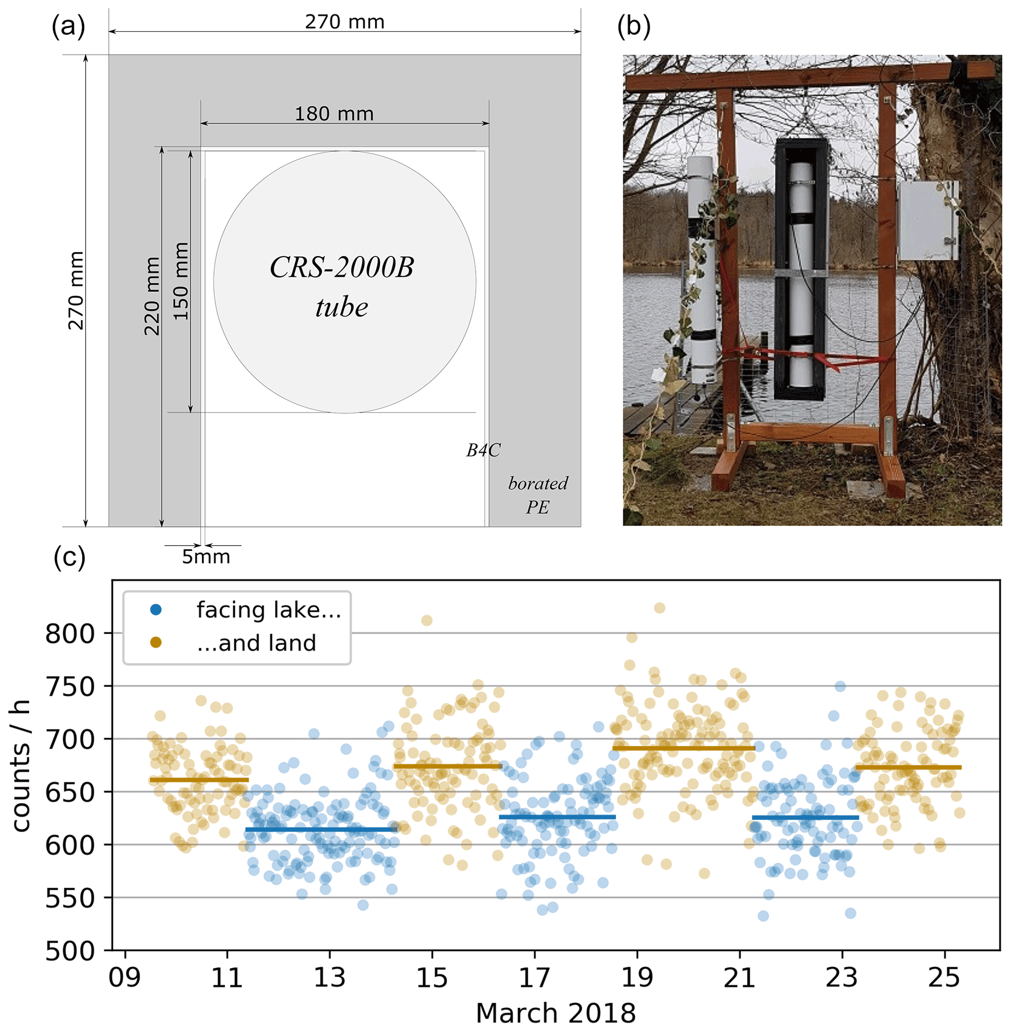
Figure 1 CRNS sensor prototype with directional shielding, operated with alternating orientation towards a lake and land. (a) Horizontal cross section. (b) Installation with directional control; here, the unshielded direction is oriented towards the viewer, i.e. the land site. The white box on the right contains the logger and modem. A conventional bare counting tube is mounted to the left. (c) Pilot measurement at a shore with alternating orientation towards the lake vs. land area, as half-planes (cf. Fig. 3). Dots represent values for 30 min aggregation.

1.3 Uncertainty in CRNS measurements

The neutron count rate R [counts h⁻¹] registered by a detector is a function of the incoming neutron flux, detector sensitivity and hydrogen pools in its footprint. Assuming a stationary setting of these factors and disregarding all errors and uncertainties, this corresponds to an expected value of total counted neutrons N [counts] in a measurement period of Δt [h] of

$$\begin{array}{}\text{(2)}& N=R\cdot \mathrm{\Delta }t.\end{array}$$

However, when dealing with real measured neutron counts N, two sources deteriorating the signal must be considered: (1) statistical error of counts and (2) device noise and/or unintended counts.

1. Due to the stochastic nature of the counting process, the number of neutrons N (i.e. the realization of a measurement) is subject to a Poisson-type error σ. From the Poisson characteristics of the counting process, it follows that

   $$\begin{array}{}\text{(3)}& \mathit{\sigma }=\sqrt{N},\end{array}$$

   with σ being the standard deviation of all the values of N we would get when repeating the measurement in the given interval.

2. A typical CRNS detector is targeted at counting epithermal neutrons (0.5 eV < E < 10⁵ eV, Köhli et al., 2018), because these neutrons show sensitivity to the abundance of hydrogen within the footprint. However, the counting is affected by additional untargeted neutron counts N_!epi, e.g. caused by ionizing particles from other energy levels, terrestrial radiation and background radioactivity of detector materials (Weimar et al., 2020). N_!epi is associated with an error of σ_!epi. Thus, the overall uncertainty σ_total when measuring N_total is a superposition of the two error sources.

The above-mentioned errors can be characterized by appropriate distributions and their respective parameters.

Concerning neutrons counted of other energy levels N_!epi, the measured signal contains a fraction ϵ of such “bycatch” flux. For a typical gas detector, ϵ results from approximately 20 % thermal and 10 % counts from fast neutrons (Baatz et al., 2015; Köhli et al., 2021) in the measured signal (the precise values depend on ambient hydrogen pools and chosen cutoff thresholds). Consequently, the actual number of counted neutrons N_total is

$$\begin{array}{}\text{(4)}& N_{\mathrm{total}}=N_{\mathrm{epi}}+N_{\mathrm{!}\mathrm{epi}}=N_{\mathrm{epi}}+\mathit{ϵ}\cdot N_{\mathrm{total}}={\displaystyle \frac{\mathrm{1}}{\mathrm{1}-\mathit{ϵ}}}{N}_{\mathrm{epi}},\end{array}$$

where ϵ is the fraction of bycatch neutrons.

Analogously to Eq. (3), the respective additional noise introduced with N_!epi is

$$\begin{array}{}\text{(5)}& {\mathit{\sigma }}_{\mathrm{!}\mathrm{epi}}=\sqrt{N_{\mathrm{!}\mathrm{epi}}}=\sqrt{{\displaystyle \frac{\mathit{ϵ}}{\mathrm{1}-\mathit{ϵ}}}\cdot N_{\mathrm{epi}}}.\end{array}$$

According to our measurements, counts caused by radioisotope contamination of the detector walls are on the order of 0.5 $\mathrm{counts}{\mathrm{h}}^{-\mathrm{1}}{\mathrm{m}}^{-\mathrm{2}}$ of the proportional counter (cf. Dębicki et al., 2011, for comparable tubes). This amounts to approximately 0.5 counts h⁻¹ for a standard CRS1000. Like other counts of unintended ionizing radiation (detector gas, protons and muons, etc.), these can be effectively filtered out by appropriate detector threshold settings in the electronics (Quaesta Instruments, Gary Womack, personal communication, 2020) and are thus ignored here. We also consider temperature effects (reported for neutron monitors, e.g. by Krüger et al., 2008) as negligible, as we are dealing with a pairwise concomitant operation (see Fig. 3), in which such effects would be cancelled out. Noise from electronic components (e.g. from external fields) is on the order of <10 counts h⁻¹ for typical detectors and can be effectively eliminated with appropriate threshold settings (Quaesta Instruments, Gary Womack, personal communication, 2020). Thus, it is also ignored here.

1.4 Specific challenges with directional neutron sensing in CRNS

Generally, CRNS measurements are affected by the uncertainties described in Sect. 1.3. For directional CRNS measurements, additional challenges arise:

• Incoming cosmogenic fast neutrons are converted to epithermal neutrons by hydrogen pools within the footprint. In this context, we denote the location of this conversion as “origin”, as it constitutes the place for which we infer the information when measuring the neutron. However, most of these epithermal neutrons do not reach the sensor directly. Instead, neutrons arriving at the sensor have usually experienced multiple elastic collisions, resulting in an irregular trajectory. This phenomenon is especially pronounced for origins far from the sensor. Consequently, the incidence angle of a neutron reaching the detector is less correlated with its angle of origin the farther the distance between origin and detector. Thus, a directional shielding can only imperfectly filter epithermal neutrons for their direction of origin.

• A directional shielding blocks neutrons reaching the detector from certain angles. This blockage can be achieved by a sufficiently thick blocking material, e.g. layers of high-density polyethylene (HDPE). For practical reasons, however, compromises between blocking properties and constraints in size or weight have to be made. Thus, the directional blocking will be imperfect, allowing a certain fraction of neutrons to reach the detector also from the shielded side.

• Blocking neutrons arriving at the detector from certain angles effectively reduces the overall count rate. Consequently, longer integration times are required for obtaining the same number of counts by a given sensor in a given environment.

Directional neutron sensing aims to determine the neutron flux rate R₁ that is characteristic of the area A₁ in the field of view (see Fig. 3). The flux rate R₂ of the complementary area A₂ may also be of interest in itself or effectively only be a factor influencing the measurement. The signal contrast between the two, i.e. the relative difference in the two flux rates (ΔR; see Eq. 19) is eventually determined by the different hydrogen inventories in the two areas.

Summarizing the general uncertainties (Sect. 1.3) and the limitations specific to directional measurements, we may conceptualize the determination of these pools via directional neutron measurement of R₁ (and R₂) as a trade-off problem with the parameters count rate (R₁), the signal contrast (ΔR) and the aggregation time (Δt): to obtain measurements for R₁ at a given accuracy, two of these parameters (e.g. count rate and signal contrast) determine the minimum of the third parameter (e.g. aggregation time; see Fig. 2). If we raise the required accuracy, the lower limits of the three parameters need to be increased (greyed-out areas in Fig. 2). The same applies if the relative noise of the measurement increases (e.g. by a higher device noise or a narrower shielding angle).

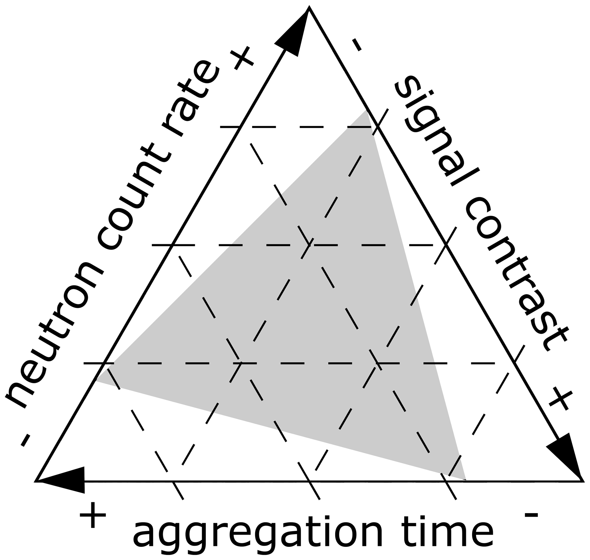
Figure 2 “Tradeoff-triangle” in directional CRNS measurements as ternary plot: for a given combination of two of these parameters, the third parameter must be adjusted accordingly to obtain the requested accuracy. The inner triangle (grey) illustrates the parameter space for an increase in required accuracy. The straight outline here is only chosen for the sake of simplicity and could be curved instead.

Systematically exploring these dependencies and limitations is a prerequisite for the design and application of directional CRNS measurements. However, in situ experiments are difficult to implement, as they require well-defined setups with spatially known neutron flux rates and multiple configurations of sensors and shielding. Instead, we propose to use simulations of neutron scattering and neutron detection in order to better understand and quantify potentials and limitations of directional CRNS measurements. Our specific objectives are as follows:

1. Quantify directional specificity and reduction in neutron count of a directional CRNS sensor setup.

2. Assess the informative value of directional CRNS measurements as a function of signal aggregation time, count rates, signal contrast and sensor noise and the respective limits of applicability.

Objective 2 can be addressed from different perspectives:

• A.

  What temporal resolution Δt could be obtained?

• B.

  What spatial contrast in the count rates ΔR can be resolved?

• C.

  What count rates R are required to yield robust estimates?

Each of these points (A–C) can be addressed when looking at either (I) determining count rates at a chosen accuracy or (II) statistically distinguishing two count rates. These are somewhat different objectives with different requirements, which will be further demonstrated in the results section.

2 Methods and data

By applying the neutron simulation model URANOS (Ultra Rapid Neutron-Only Simulation) (Sect. 2.1.1), we assess the characteristics of angular shielding (Sect. 2.1.2). As these simulations are computationally demanding, we then generalize the findings in an analytical approach (Sect. 2.2) in order to outline the possible range of application of directional CRNS measurements. This assessment exploits two extreme scenarios, termed “favourable” and “unfavourable”, encompassing the most beneficial and most adverse settings, respectively.

2.1 Neutron simulation

2.1.1 Neutron simulation model URANOS

The Monte Carlo tool URANOS (Köhli et al., 2015) is designed specifically for modelling neutron interactions within the environment in the framework of CRNS. The standard calculation routine features a ray-casting algorithm for a single neutron propagation and a voxel engine. Instead of propagating particle showers in atmospheric cascades, URANOS reduces the computational effort and makes use of the analytically defined cosmic-ray neutron spectrum by Sato (2015). The URANOS model can use setups with either open domains of at least 600 m or smaller sizes with periodic or reflecting boundary conditions.

2.1.2 Setups simulated with URANOS

The simulation geometry consists of a ground layer with a thickness of 1.3 m and a 1000 m air (buffer) layer. The soil consists of 50 %_Vol solids and a scalable amount of H₂O. The solids are composed of 75 %_Vol SiO₂ and 25 %_Vol Al₂O₃ at a particle density of 2.86 g cm⁻³. The air medium consists of 78 %_Vol nitrogen, 21 %_Vol oxygen and 1 %_Vol argon at a pressure of 1020 mbar. The air humidity is set to 7 g m⁻³ and soil moisture is set to 10 %_Vol. In this study, three different simulation setups have been used:

1. In order to assess the effect the additional moderating effect of the directional shielding on the measured intensity, in a first setup, the detector with its actual dimensions has been placed inside a domain of 10 m lateral extension with periodic boundaries and a cosmic neutron source.

2. Secondly, the to-scale model of the detector has been used to calculate the response function (Köhli et al., 2018) of each face of the detector by probing the response to a series of monoenergetic neutrons released perpendicular to its face.

3. Thirdly, a virtual detector has been placed in a large-size domain. This entity was equipped with the beforehand-found response functions and had, in order to collect enough statistics, a geometry which is slightly larger than the physical instrument. This can be regarded as a suitable approximation for the purpose of investigating the distance-dependent angular response. This spherical virtual detector has been placed at a height of 1.75 m with a radius of 1.25 m within a domain size of 800 m × 800 m. Cosmic neutrons are released at a height of 50 m using a circular source with a radius of 400 m. Thermal neutron transport was disabled for reasons of computational speed (please note that their effect on signal noise is still included in the generalization of the simulation, Sect. 2.2). This configuration leads to a homogeneous neutron flux distribution within the innermost 400 m × 400 m. Origin data can be retrieved for a radius of approximately 300 m.

2.2 Generalization of interpreting directional measurements

Aiming to generalize the findings of the neutron simulations (Sect. 3.1.2 and 3.1.3), we conceptualize the directional measurement as a linear mixing and analytically express the corresponding propagation of errors for an simplistic geometric setup. This analytical approach allows us to assess the feasibility of directional CRNS in a wide range of settings without the need to perform numerous computationally demanding numerical simulations.

2.2.1 Description of idealized geometric setup

For the sake of simplicity, we use the simplest geometric setup imaginable for directional CRNS measurements: a plain divided into two homogeneous half-spaces (A₁ and A₂). Each half-space corresponds to a count rate R₁ and R₂, respectively, when measured far enough from its borders. At the border of both half-spaces, we implement a directional detector. When facing A₁, it yields the count rate R_f1; when directed towards A₂, it registers the count rate R_f2. Both count rates are measured and used in the computations. Consequently, the evaluation employs a FOV of 180^∘ (π). This value has no direct relation to the geometry of the opening face of the shielding, which is apparently somewhat narrower. Instead, it is an arbitrary decision to target this area within the FOV with the measurement.

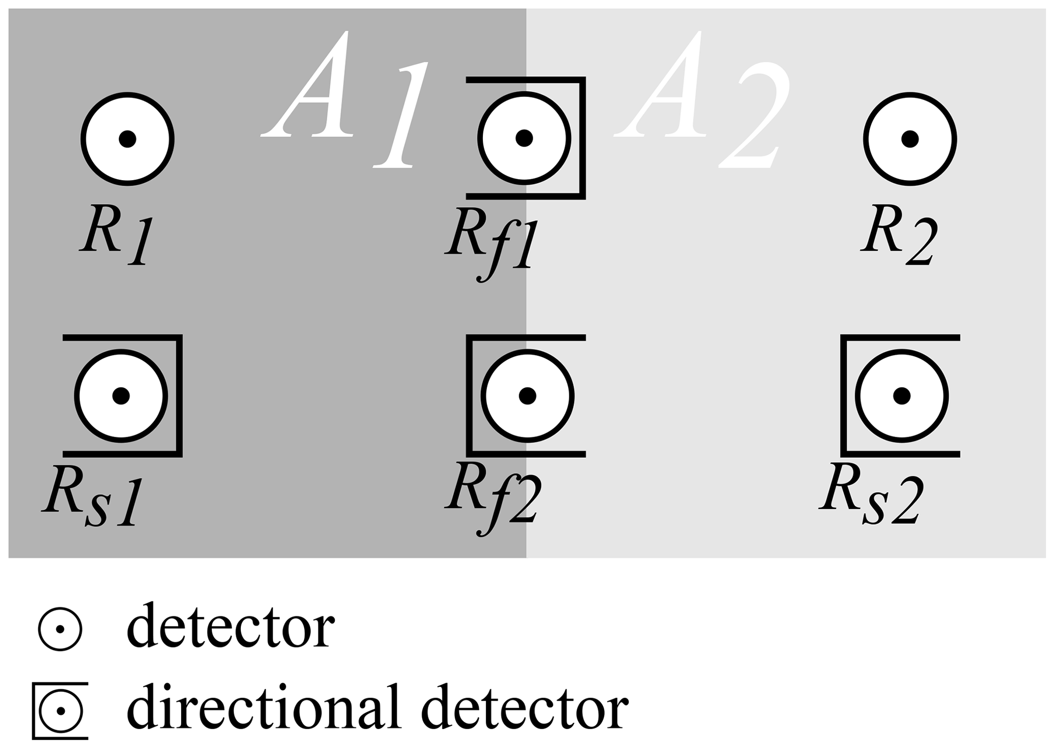
Figure 3 Geometric setup of experiment: R₁ and R₂ denote the CRNS count rates within the half-planes A₁ and A₂, respectively. R_s1 and R_s2 symbolize the operation with directional shielding (creating a “directional CRNS sensor”). R_f1 and R_f2 denote the count rates the directional sensor registers when placed on the border and pointed towards A₁ or A₂, respectively.

2.2.2 Components of the CRNS signal

The total count rate R_total registered by a sensor results from non-epithermal and epithermal neutrons (see Eq. 4).

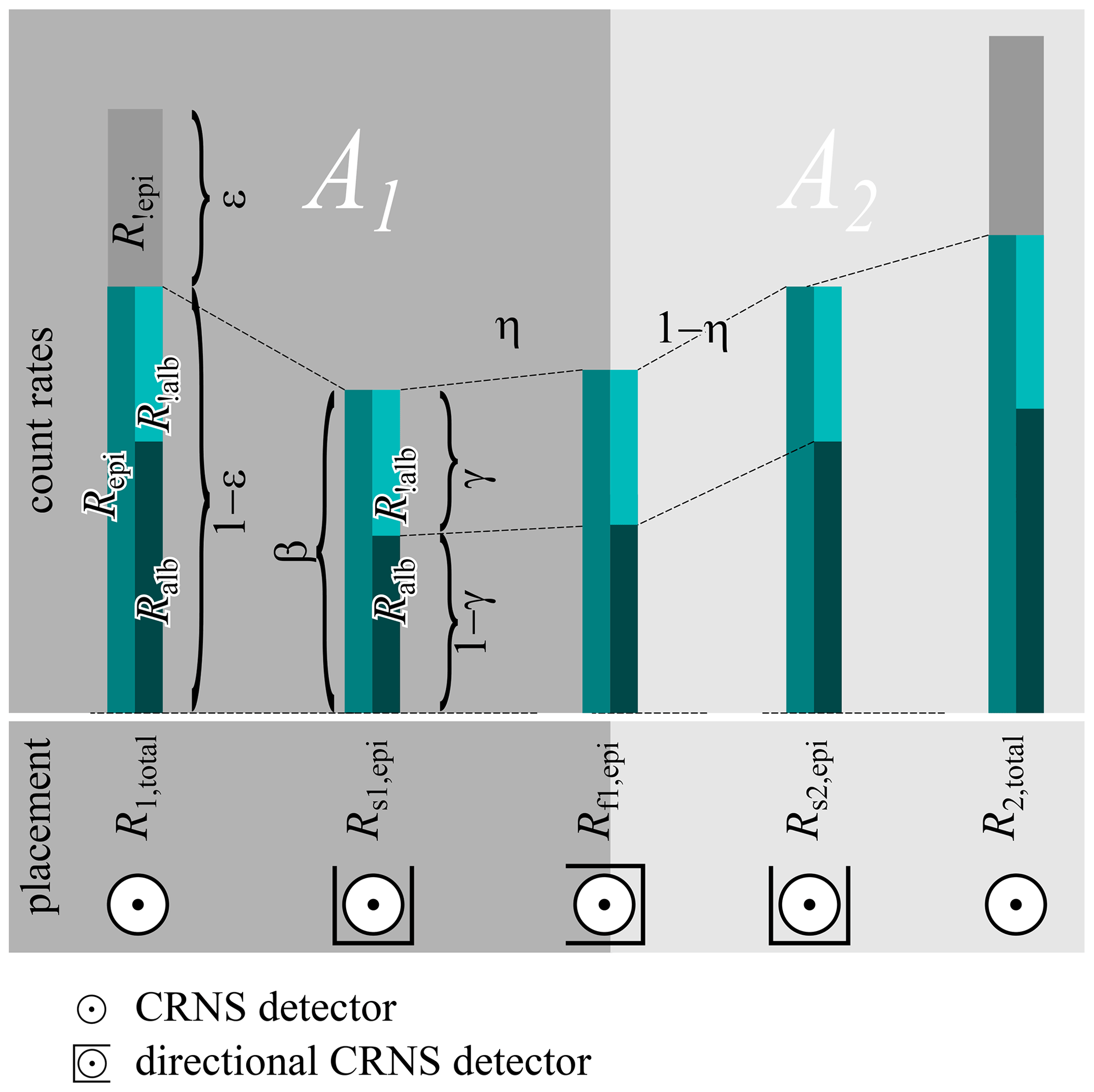
Figure 4 Components of a CRNS signal for omnidirectional and directional detectors. Left bar: partitioning of the total count rate (R_total) into spurious R_non-epi and counts of epithermal neutrons (R_epi), in turn resulting from albedo (R_alb) and non-albedo (R_non-alb) neutrons. Second bar: reduced count rate R_s and increase of no-albedo fraction γ by adding the directional shielding. Third bar: mixing of signal with directional detector placed between the half-planes A₁ and A₂.

The epithermal counts, in turn, are composed of counts from albedo neutrons having interacted with the hydrogen pools of interest (R_alb) and non-albedo neutrons (R_non-alb) without such interaction. We denote the respective percentage as γ (see Fig. 4, left bar), so

$$\begin{array}{}\text{(6)}& R_{\mathrm{alb}}=(\mathrm{1}-\mathit{\gamma })\cdot R_{\mathrm{epi}}.\end{array}$$

Note that γ differs between the omnidirectional and the directional detector, which will be shown later. Therefore, we distinguish in the following between a γ_D and a γ_!D for the directional and the omnidirectional detector, respectively.

For the directional sensor placed entirely into the interior of one of the half-planes, A₁ or A₂, the directional shielding causes partial blockage of the neutrons arriving, reducing its count rate by the factor β to R_s (see Fig. 4, second bar):

$$\begin{array}{}\text{(7)}& R_{\mathrm{s},\mathrm{epi}}=\mathit{\beta }\cdot R_{\mathrm{epi}}.\end{array}$$

Values for γ and β were obtained from neutron simulations as discussed in Sect. 2.1.2, setup 1.

2.2.3 Mixing and unmixing of signals from directional sensors

When placing the directional sensor exactly between the two half-planes A₁ and A₂, the components of its counts (albedo and non-albedo) can be described as a mixing from the adjacent planes. The albedo neutrons mix according to the orientation of the shielding and the respective directional contribution η (Eq. 1), i.e. the ratio between counts from the desired angle and total counts (see Fig. 4, third bar):

$$\begin{array}{}\text{(8a)}& {\displaystyle }{R}_{\mathrm{f}\mathrm{1},\mathrm{alb}}& {\displaystyle }=\mathit{\eta }\cdot R_{\mathrm{s}\mathrm{1},\mathrm{alb}}+(\mathrm{1}-\mathit{\eta })\cdot R_{\mathrm{s}\mathrm{2},\mathrm{alb}}\text{(8b)}& {\displaystyle }{R}_{\mathrm{f}\mathrm{2},\mathrm{alb}}& {\displaystyle }=\mathit{\eta }\cdot R_{\mathrm{s}\mathrm{2},\mathrm{alb}}+(\mathrm{1}-\mathit{\eta })\cdot R_{\mathrm{s}\mathrm{1},\mathrm{alb}}.\end{array}$$

The directional detector may be oriented towards the left half-plane A₁ or the right half-plane A₂. Formally, there is no fundamental difference in the equations for each, and we exemplify the next step with the one oriented towards A₁ and its count rate R_f1,alb.

Substituting Eq. (8a) with Eqs. (6), (7) and then (4) yields

$$\begin{array}{}\text{(9)}& \begin{array}{rlrl}{R}_{\mathrm{f}\mathrm{1},\mathrm{alb}}& =(\mathrm{1}-{\mathit{\gamma }}_{\mathrm{s}})& (\mathit{\eta }\cdot R_{\mathrm{s}\mathrm{1},\mathrm{epi}}& +(\mathrm{1}-\mathit{\eta })\cdot R_{\mathrm{s}\mathrm{2},\mathrm{epi}})\\ & =(\mathrm{1}-{\mathit{\gamma }}_{\mathrm{s}})\cdot \mathit{\beta }& (\mathit{\eta }\cdot R_{\mathrm{1},\mathrm{epi}}& +(\mathrm{1}-\mathit{\eta })\cdot R_{\mathrm{2},\mathrm{epi}})\\ & =(\mathrm{1}-{\mathit{\gamma }}_{\mathrm{s}})\cdot \mathit{\beta }\cdot (\mathrm{1}-\mathit{ϵ})& (\mathit{\eta }\cdot R_{\mathrm{1},\mathrm{total}}& +(\mathrm{1}-\mathit{\eta })\cdot R_{\mathrm{2},\mathrm{total}}).\end{array}\end{array}$$

Considering both rates R_f1,alb and R_f2,alb simultaneously in a vector R_f,alb, we may write in matrix notation:

$$\begin{array}{}\text{(10)}& \begin{array}{rl}{\mathit{R}}_{\mathrm{f},\mathrm{alb}}& =\left(\begin{array}{c}{R}_{\mathrm{f}\mathrm{1},\mathrm{alb}}\\ R_{\mathrm{f}\mathrm{2},\mathrm{alb}}\end{array}\right)\\ & =(\mathrm{1}-{\mathit{\gamma }}_{\mathrm{s}})\cdot \mathit{\beta }\cdot (\mathrm{1}-\mathit{ϵ})\cdot \left(\begin{array}{cc}\mathit{\eta }& \mathrm{1}-\mathit{\eta }\\ \mathrm{1}-\mathit{\eta }& \mathit{\eta }\end{array}\right)\left(\begin{array}{c}{R}_{\mathrm{1},\mathrm{total}}\\ R_{\mathrm{2},\mathrm{total}}\end{array}\right)\\ & =(\mathrm{1}-{\mathit{\gamma }}_{\mathrm{s}})\cdot \mathit{\beta }\cdot (\mathrm{1}-\mathit{ϵ})\cdot \mathbf{A}\cdot {\mathit{R}}_{\mathrm{total}},\end{array}\end{array}$$

where A is a symmetric matrix containing the coefficients for the mixing. For the non-albedo neutrons R_f,non-alb, the mixing is simply the average of the corresponding rates:

$$\begin{array}{}\text{(11)}& \begin{array}{rl}{\mathit{R}}_{\mathrm{f},\mathrm{!}\mathrm{alb}}& ={\displaystyle \frac{\mathrm{1}}{\mathrm{2}}}\cdot \mathbf{J}\cdot {\mathit{R}}_{\mathrm{D},\mathrm{!}\mathrm{alb}}={\displaystyle \frac{\mathrm{1}}{\mathrm{2}}}\cdot \mathbf{J}\cdot {\mathit{\gamma }}_{\mathrm{s}}{\mathit{R}}_{\mathrm{D},\mathrm{epi}}\\ & ={\displaystyle \frac{\mathrm{1}}{\mathrm{2}}}\cdot \mathbf{J}\cdot {\mathit{\gamma }}_{\mathrm{s}}\cdot \mathit{\beta }{\mathit{R}}_{\mathrm{epi}}\\ & ={\displaystyle \frac{\mathrm{1}}{\mathrm{2}}}\cdot \mathbf{J}\cdot {\mathit{\gamma }}_{\mathrm{s}}\cdot \mathit{\beta }\cdot (\mathrm{1}-\mathit{ϵ}){\mathit{R}}_{\mathrm{total}},\end{array}\end{array}$$

where J is the matrix of ones.

Applying Eq. (4) for the non-epithermal counts leads to

$$\begin{array}{}\text{(12)}& \begin{array}{rl}{\mathit{R}}_{\mathrm{f},\mathrm{!}\mathrm{epi}}& ={\displaystyle \frac{\mathit{ϵ}}{\mathrm{1}-\mathit{ϵ}}}\cdot {\mathit{R}}_{\mathrm{f},\mathrm{epi}}={\displaystyle \frac{\mathit{ϵ}}{\mathrm{1}-\mathit{ϵ}}}\cdot \left({\mathit{R}}_{\mathrm{f},\mathrm{alb}}+{\mathit{R}}_{\mathrm{f},\mathrm{!}\mathrm{alb}}\right)\\ & =\mathit{ϵ}\cdot \mathit{\beta }\cdot \left((\mathrm{1}-{\mathit{\gamma }}_{\mathrm{s}})\cdot \mathbf{\text{A}}+{\displaystyle \frac{\mathrm{1}}{\mathrm{2}}}\cdot \mathbf{J}\cdot {\mathit{\gamma }}_{\mathrm{s}}\right){\mathit{R}}_{\mathrm{total}}.\end{array}\end{array}$$

Adding Eqs. (10), (11) and (12) yields the total count rates of the directional detector R_f,total:

$$\begin{array}{}\text{(13)}& \begin{array}{rl}{\mathit{R}}_{\mathrm{f},\mathrm{total}}& ={\mathit{R}}_{\mathrm{f},\mathrm{alb}}+{\mathit{R}}_{\mathrm{f},\mathrm{!}\mathrm{alb}}+{\mathit{R}}_{\mathrm{f},\mathrm{!}\mathrm{epi}}\\ & =(\mathrm{1}-\mathit{ϵ})\cdot \mathit{\beta }\cdot \left(\right(\mathrm{1}-{\mathit{\gamma }}_{\mathrm{s}})\cdot \mathbf{A}+{\displaystyle \frac{\mathrm{1}}{\mathrm{2}}}\cdot \mathbf{J}\cdot {\mathit{\gamma }}_{\mathrm{s}}\\ & +{\displaystyle \frac{\mathit{ϵ}}{\mathrm{1}-\mathit{ϵ}}}\left((\mathrm{1}-{\mathit{\gamma }}_{\mathrm{s}})\cdot \mathbf{A}+{\displaystyle \frac{\mathrm{1}}{\mathrm{2}}}\cdot \mathbf{J}\cdot {\mathit{\gamma }}_{\mathrm{s}}\right)){\mathit{R}}_{\mathrm{total}}\\ & =\left(\mathbf{A}(\mathit{\beta }-\mathit{\beta }{\mathit{\gamma }}_{\mathrm{s}})+{\displaystyle \frac{\mathrm{1}}{\mathrm{2}}}\mathit{\beta }{\mathit{\gamma }}_{\mathrm{s}}\mathbf{J}\right){\mathit{R}}_{\mathrm{total}}=\mathbf{B}{\mathit{R}}_{\mathrm{total}}\end{array},\end{array}$$

with B being a matrix summarizing all the operations.

For reconstructing the unshielded count rates in the half-spaces (R_total) from the two directional measurements (R_f1 and R_f2), we use the inverse operation:

$$\begin{array}{}\text{(14)}& {\mathit{R}}_{\mathrm{r},\mathrm{total}}={\mathbf{B}}^{-\mathrm{1}}{\mathit{R}}_{\mathrm{f}}={\displaystyle \frac{\mathrm{1}}{k_{\mathrm{1}}}}\left(\begin{array}{cc}{k}_{\mathrm{2}}& k_{\mathrm{2}}+\mathrm{2}\\ k_{\mathrm{2}}+\mathrm{2}& k_{\mathrm{2}}\end{array}\right){\mathit{R}}_{\mathrm{f},\mathrm{total}},\end{array}$$

where

$$\begin{array}{}\text{(15)}& k_{\mathrm{1}}=\mathrm{2}\mathit{\beta }(\mathrm{2}{\mathit{\gamma }}_{\mathrm{s}}\mathit{\eta }-{\mathit{\gamma }}_{\mathrm{s}}-\mathrm{2}\mathit{\eta }+\mathrm{1}),k_{\mathrm{2}}=(\mathrm{2}{\mathit{\gamma }}_{\mathrm{s}}\mathit{\eta }-{\mathit{\gamma }}_{\mathrm{s}}-\mathrm{2}\mathit{\eta }).\end{array}$$

The subscript “r” in Eq. (14) denotes the reconstructed rates for estimating the true (and unknown) ones in the half-spaces (R₁ and R₂).

2.2.4 Description of error propagation

As described in Sect. 1.3, the errors in neutron counts follow a Poisson distribution. In this study, we exclusively consider large numbers for values of N (i.e. N≫20, which is consistent with practical CRNS applications). As a consequence of the central limit theorem, we can approximate the errors with a Gaussian distribution and corresponding standard deviations:

$$\begin{array}{}\text{(16)}& P\left(\mathit{\lambda }\right)\sim \mathcal{N}(\mathit{\mu }=\mathit{\lambda },{\mathit{\sigma }}^{\mathrm{2}}={\mathit{\lambda }}^{\mathrm{2}}).\end{array}$$

As the considered errors in the two directional counts (N_f1 and N_f2) are independent, the superposition of these errors can be described based on Gaussian error propagation:

$$\begin{array}{}\text{(17)}& {\mathit{\sigma }}_F=\sqrt{{\left({\displaystyle \frac{\partial F}{\partial x}}\right)}^{\mathrm{2}}{\mathit{\sigma }}_x^{\mathrm{2}}+{\left({\displaystyle \frac{\partial F}{\partial y}}\right)}^{\mathrm{2}}{\mathit{\sigma }}_y^{\mathrm{2}}},\end{array}$$

where F denotes a function combining the contributions of x and y. In our case, F would be the reconstruction of the count rates from the directional counts (i.e. Eq. 14).

When reconstructing the rates in the half-spaces R₁ and R₂ as described in Eq. (14) and propagating the errors in both directional counts (see Eq. 17), and performing substitutions (Eqs. 4 and 13), the error in the reconstructed epithermal counts is

$$\begin{array}{}\text{(18)}& \begin{array}{rl}{\mathit{\sigma }}_{\mathrm{r},\mathrm{total}}& ={\sqrt{{\left({\mathbf{B}}^{-\mathrm{1}}\right)}^{\circ \mathrm{2}}{\mathit{\sigma }}_{\mathrm{f},\mathrm{total}}^{\circ \mathrm{2}}}}^{\circ }\\ & ={\sqrt{{\left({\mathbf{B}}^{-\mathrm{1}}\right)}^{\circ \mathrm{2}}{\sqrt{{\mathit{N}}_{\mathrm{f},\mathrm{total}}}}^{\circ \circ \mathrm{2}}}}^{\circ }\\ & ={\sqrt{{\left({\mathbf{B}}^{-\mathrm{1}}\right)}^{\circ \mathrm{2}}\mathbf{B}{\mathit{N}}_{\mathrm{total}}}}^{\circ }.\end{array}\end{array}$$

(^∘ denotes the Hadamard operations; i.e. the square and square root operation are applied element-wise on the vectors and matrices.)

2.2.5 Determining and distinguishing neutron count rates

As mentioned in Sect. 1.2, directional CRNS is motivated by two aims:

• I.

  determining the neutron count rate for the area the detector is directed at (optionally, also the rate for the complementary area) and

• II.

  distinguishing the count rates of the two areas, i.e. detecting a difference in neutron flux.

Both aims can be pursued jointly or separately; however, achieving one does not necessarily guarantee achieving the other. For example, it might be possible to determine two count rates with high precision, but nevertheless it might be impossible to detect a significant difference between them, when they are (nearly) equal. Conversely, very dissimilar count rates can be discerned, even if their actual value cannot be determined very precisely. Therefore, we look at both of these aims separately. We formalize the determination of count rates (aim I) as being able to confine their 95 %confidence interval (CI) to a value smaller than a desired precision, expressed as a fraction of the actual value. We chose a value of 5 % for our illustrations, which roughly corresponds to an error of 2 %-points in volumetric water content for the conversion used by Fersch et al. (2020). For distinguishing two count rates (aim II), we propose they are significantly different, if their difference – regarding the associated uncertainties – is statistically different from 0 with a chosen p value (0.05 in our case).

2.2.6 Selected example values chosen in the analysis

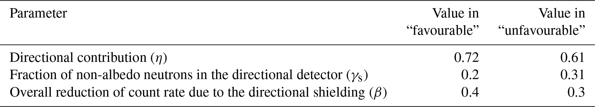
Applying Eq. (18), e.g. using provided R code, the described analysis can be performed for any combination of parameters of interest, i.e. count rates (R₁, R₂) or their respective contrast (ΔR), temporal resolution (Δt), directional contribution (η), overall reduction of count rate due to the directional shielding (β) and the fraction of bycatch neutrons (ϵ). However, for illustrative purposes, in the results section (Sect. 3.2), we provide some example plots trying to capture the typical ranges of the parameters involved. The parameters η, γ_s and β were set to extreme values and combined in two scenarios termed “favourable” and “unfavourable”, encompassing the most favourable and most adverse settings, respectively (see Table 1). The other parameters are varied continuously along a range. This selection was guided by a range of diverse settings found in the literature summarized in Table 2. Detailed explanations are given in the following.

Fraction of non-epithermal counts (ϵ): in the examples, we illustrate the situation for an “favourable” scenario assuming a low fraction of non-epithermal counts (ϵ=0.1) and for a “unfavourable” setting (ϵ=0.3).

Directional contribution (η): the effect of the directional shielding is expressed by the directional contribution η, i.e. the ratio between the counts from the area targeted and total counts (see Eq. 1). In the displayed examples, we only consider symmetrical half-planes (see Fig. 3 for the “favourable” scenario with the perfect shielding (η=0.72) and the “unfavourable” implementation of the actual shielding (η=0.61) as resulted from the neutron simulations (see Sect. 3.1.3, Table 3).

Fraction of non-albedo neutrons in the directional detector (γ_s): the fraction of non-albedo neutrons, i.e. those without the interaction with the surface, is a function of the hydrogen inventory in the footprint. We estimate respective values based the neutron simulations (see Sect. 3.1.3). For the “favourable” scenario, we choose a low value (γ_s=0.2) corresponding to very dry conditions; the “unfavourable” implementation (γ_s=0.31) mimics a very wet environment (see Sect. 3.1.3 and Table 3).

Overall reduction of count rate due to the directional shielding (β): the directional shielding reduces the total count rate in the directional detector to the fraction β (see Eq. 7). For the “favourable” scenario, we choose a high value (β=0.4) corresponding to very wet conditions; the “unfavourable” implementation (β=0.3) mimics a very dry environment (see Sect. 3.1.3, Table 4).

Table 1 Parameter values describing the “favourable” and “unfavourable” scenarios.

The following parameters were varied along plausible ranges.

Count rate (R): count rates depend on site conditions (i.e. incoming neutrons and hydrogen pools) and detector sensitivity. We selected values of 500, 2000, 8000, 40 000 and 150 000 counts h⁻¹ as example values for the count rates registered at the detectors (R_total; see Eq. 4).

Contrast in count rates of the half-planes (ΔR): we denote the difference in the count rates in the two half-planes with ΔR, expressed as their difference relative to the lower of the two values:

$$\begin{array}{}\text{(19)}& \mathrm{\Delta }R={\displaystyle \frac{R_{\mathrm{2}}-R_{\mathrm{1}}}{R_{\mathrm{1}}}}.\end{array}$$

Information on a realistic range of this value would ideally be obtained from spatially distinct sensor locations, e.g. from roving. As this information is unavailable for most considered examples, we use the temporal variation of the signal as a proxy, resulting in example values of 0.2, 0.5, 0.8 and 1.4.

Aggregation time Δt: Schrön et al. (2018b) suggests that the typical temporal resolution of standard stationary detectors is in the range of 3 to 12 h, depending on detector technology and site conditions. Bogena et al. (2013) and Fersch et al. (2020) use longer aggregation intervals of 24 h. For our study, we display results for values of 1, 6, 12 and 24 h. Longer aggregation times are not recommended from a hydrological perspective, since they would commonly imply too high a change of the observed variable during that interval (e.g. by rainfall or drying and respective change in R).

Bogena et al. (2013)Rivera Villarreyes et al. (2011)Baroni et al. (2018)Fersch et al. (2020)Schrön et al. (2017)Fersch et al. (2020)Schattan et al. (2017)Fersch et al. (2020)Fersch et al. (2020)

Table 2 Neutron count rates reported in experimental CRNS studies. Bold entries have been approximated in the representative examples.

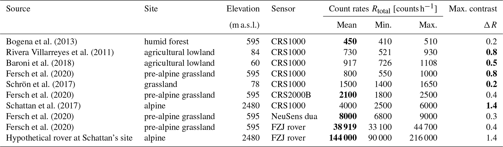
For a subsequent evaluation of the feasibility for a specific case, we use the setting listed in line 6 of Table 2, i.e. the measurement using the prototype directional detector described in Sect. 1.2 with R₁=2100 counts h⁻¹, ΔR=0.4.

3 Results and discussion

This section presents the results of the detailed numerical simulations (Sect. 3.1), followed by their generalization using the analytical approach (Sect. 3.2).

3.1 Numerical neutron simulation

3.1.1 Effect of shielding on count rates

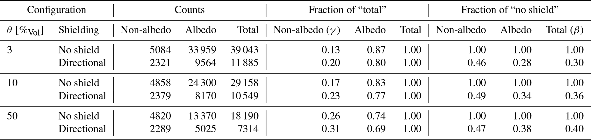
Increasing the thickness of the polyethylene shielding not only reduces the neutron flux from the non-targeted direction, it also partially reflects neutrons from the other direction and changes the energy response. Furthermore, the moderator itself produces secondary neutrons, which can be regarded as an offset bias. Thus, with the main function of blocking neutrons from the non-targeted directions, a number of secondary effects come along, which slightly change the characteristics of the CRNS probe. Table 3 summarizes the effects of adding a directional shielding to a detector. It demonstrates that the fraction of non-albedo neutrons γ is higher for the directional detector than for the unshielded operation. Furthermore, it increases with the amount of hydrogen in the footprint.

Secondly, the total count rate reduction by adding the shield β is at least 30 %. For the wetter conditions, it is even higher, reaching β=40 % for θ=50 % (see Table 3).

Table 3 Effect of directional shielding on neutron counts. Simulated counts for different configurations of volumetric soil moisture (θ) and shielding (“no shield ”/“directional”). The counts are differentiated in those with and without surface interaction (“albedo”/“non-albedo”).

3.1.2 Angular sensitivity

The CRNS method relies on the principle that the detected neutrons have interacted with the soil of the footprint – usually several times – and thus carry information about its hydrogen inventory. Due to these atmosphere–ground interface crossings, the correlation between neutron origin and field of view of the probe is diluted. Most neutron scatterings before detection are located in the direct vicinity of the detector, which to some extent dissociates the vector of detection and the vector to the origin of the neutron. For this reason, the shielding does not as effectively filter neutron vectors from remote origins, but its directional specificity is much more pronounced for neutrons with origins in the near range.

From Fig. 5, which shows the case of a detector in the “favourable” scenario, we can conclude the following: the largest part of the neutron flux remains undetected (black), due to insufficient energy or being scattered off the detector material itself. Most neutrons counted entered the instrument from a viewing angle corresponding to the open side face (orange). However, their origin only partially lies in that direction. While often being transported “geometrically” (i.e. directly) to the detector when being released from the soil in the direct vicinity of the instrument (yellow line), more distant origins tend to incur much more directional changes of the neutron. This leads to a flattened angular distribution (orange and brown lines).

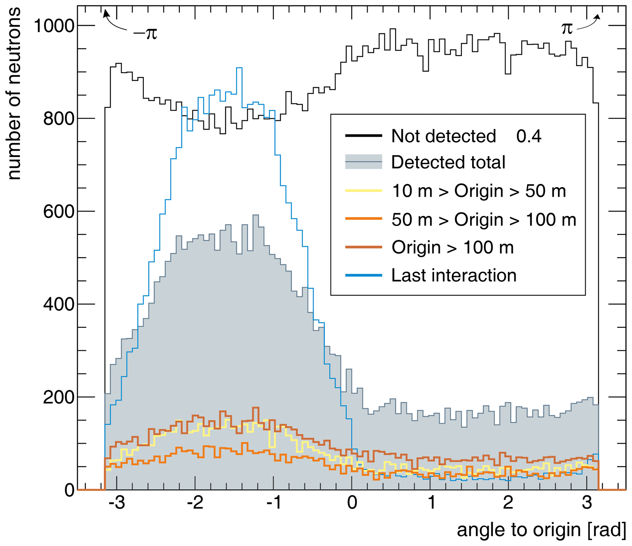
Figure 5 Neutron origin angles for the designed directional detector (shielded to all sides except the front which points to $-\mathit{\pi }/\mathrm{2}$). The range groups are defined by the distance of neutron origin to the detector, except “last interaction”, which refers to the last scattering before detection, typically in air. The distribution “not detected” refers to the total flux through the instrument; please note the different scale.

3.1.3 Shielding effect

In the “unfavourable” scenario, the insufficient shielding of MeV neutrons to the sides leads to field-of-view contamination of approximately 10 % of the signal, mostly due to the limited thickness of the HDPE shielding; see Fig. 6. Compared to the ideally shielded detector in Fig. 5, the contamination causes an increase of roughly 50 % in the plateau region of undesired angles.

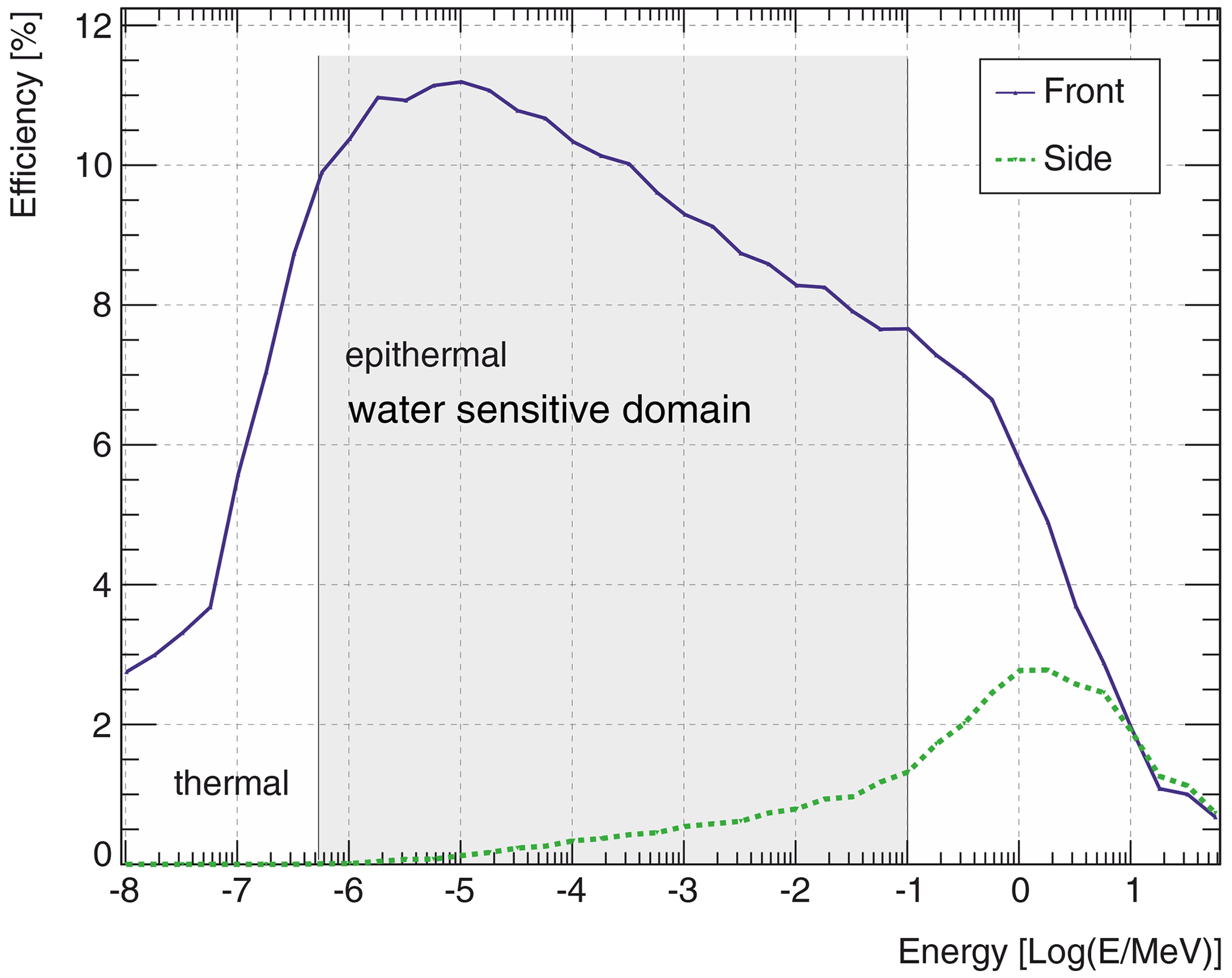
Figure 6 Energy response function of the directional detector for the open face (“front”) and a side face. The sensitivity difference between side faces and the one opposed to the open face (“back side”) is negligible.

In order to quantitatively assess the directional sensing capabilities, we use the directional contribution (see Eq. 1). We chose as representative target FOVs 90^∘ ($\mathit{\pi }/\mathrm{2}$) and 180^∘ (π). The results are summarized in Table 4. For a rather narrow viewing angle (i.e. 90^∘), even in an optimistic case, less than half of the signal originates from that direction. If the field-of-view limitation is set to a full half-space, 60 % of the signal is representative of information from those angles. As the actual detector suffers from a partial leaking-in of MeV neutrons, a near-field blur effect appears: as most neutrons from the direct vicinity are fast, the signal contamination due to insufficient shielding is to a large extent carrying information about the local area of the sensor.

Table 4 Directional contribution η for the actual detector model and an optimistic case in which the side faces are 100 % impermeable for neutrons. Compare the range groups also to Fig. 5.

3.2 Feasibility of directional CRNS measurements

Based on the presented findings of the neutron simulations, the following analysis has been made to assess the feasibility of the directional detector.

Figure 7 illustrates an example simulation ($R_{\mathrm{1},\mathrm{total}}=\mathrm{2100}$ counts h⁻¹, $R_{\mathrm{2},\mathrm{total}}=\mathrm{2520}$ counts h⁻¹, ϵ=0.3). It clearly shows how the rates of the directional sensor (R_f1,total, R_f2,total) are considerably lower due to the blocking effect of the directional shielding. Concerning the determination of rates, the confidence intervals narrow with increasing aggregation time. Notably, the CI for the reconstructed rates R_1r,total and R_2r,total is always considerably wider than their directly measured counterparts R_1,total and R_2,total. So, how much aggregation time is required to determine a count rate precisely? We define $\mathrm{\Delta }{t}_{\min }^{\mathrm{determ}}$ (arrows in Fig. 7) as the time when the CI gets smaller than the chosen precision of 5 % of the true value, i.e. 5 % relative precision. We use this time as an indicator of the time beyond which the determination of a count rate becomes reasonably accurate. As our focus is on the rates reconstructed from the directional measurements, the following statements refer to R_1r,total, the lower of the two reconstructed count rates, as it has the larger value of $\mathrm{\Delta }{t}_{\min }^{\mathrm{determ}}$ (green arrow in Fig. 8 at 36 h).

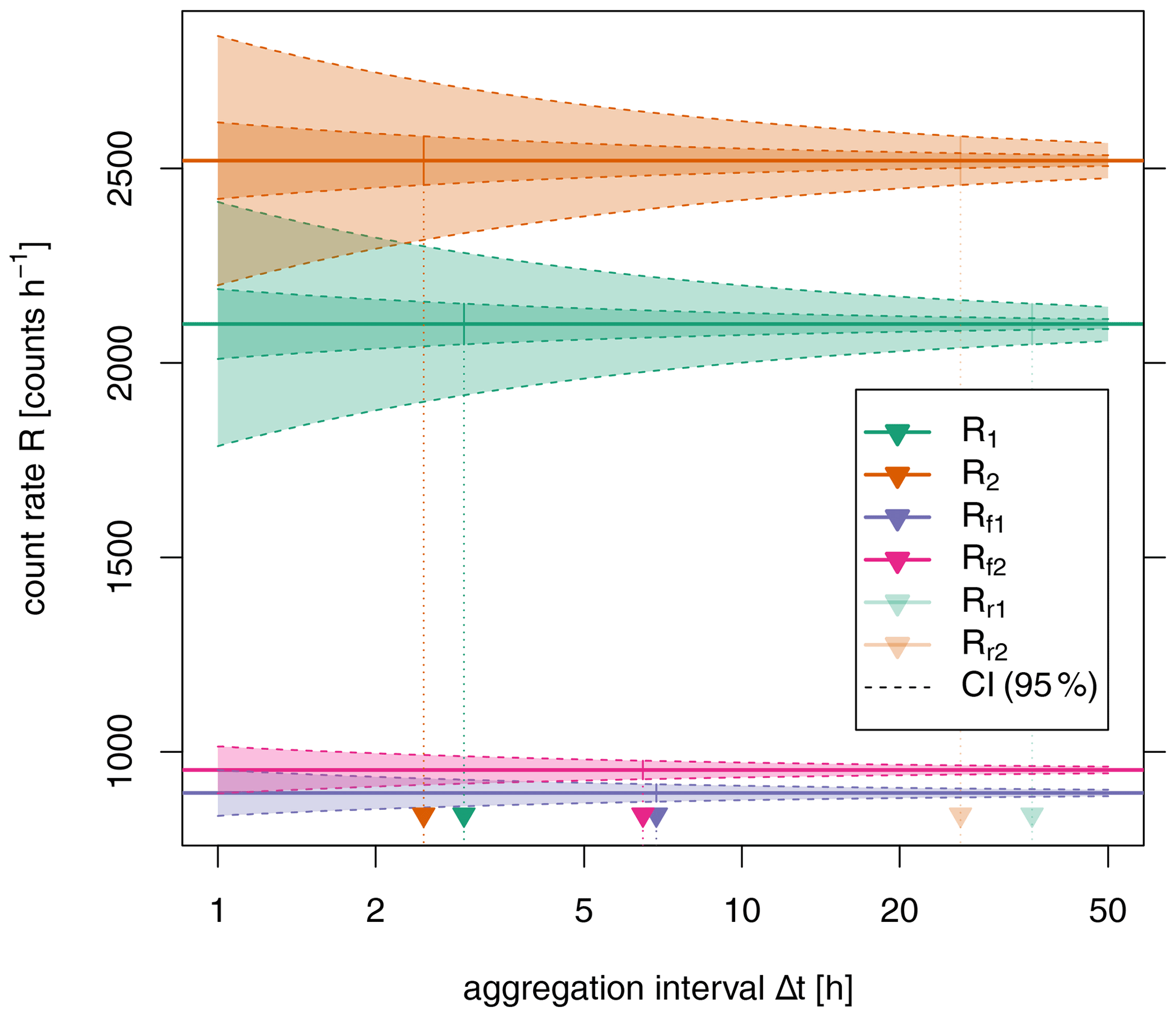
Figure 7 Example for 95 % confidence intervals for the count rates obtained within the half-spaces (R_1,total = 2100 counts h⁻¹, R_2,total = 2520 counts h⁻¹, “favourable scenario”, moderate contrast ΔR=0.2), by the directional CRNS sensors (R_f1,total, R_f2,total) and the rates reconstructed from the directional sensors (R_1r,total, R_2r,total). The vertical arrows indicate the minimum required aggregation time to confine the CI within 5 % of the true value ($\mathrm{\Delta }{t}_{\min }^{\mathrm{determ}}$).

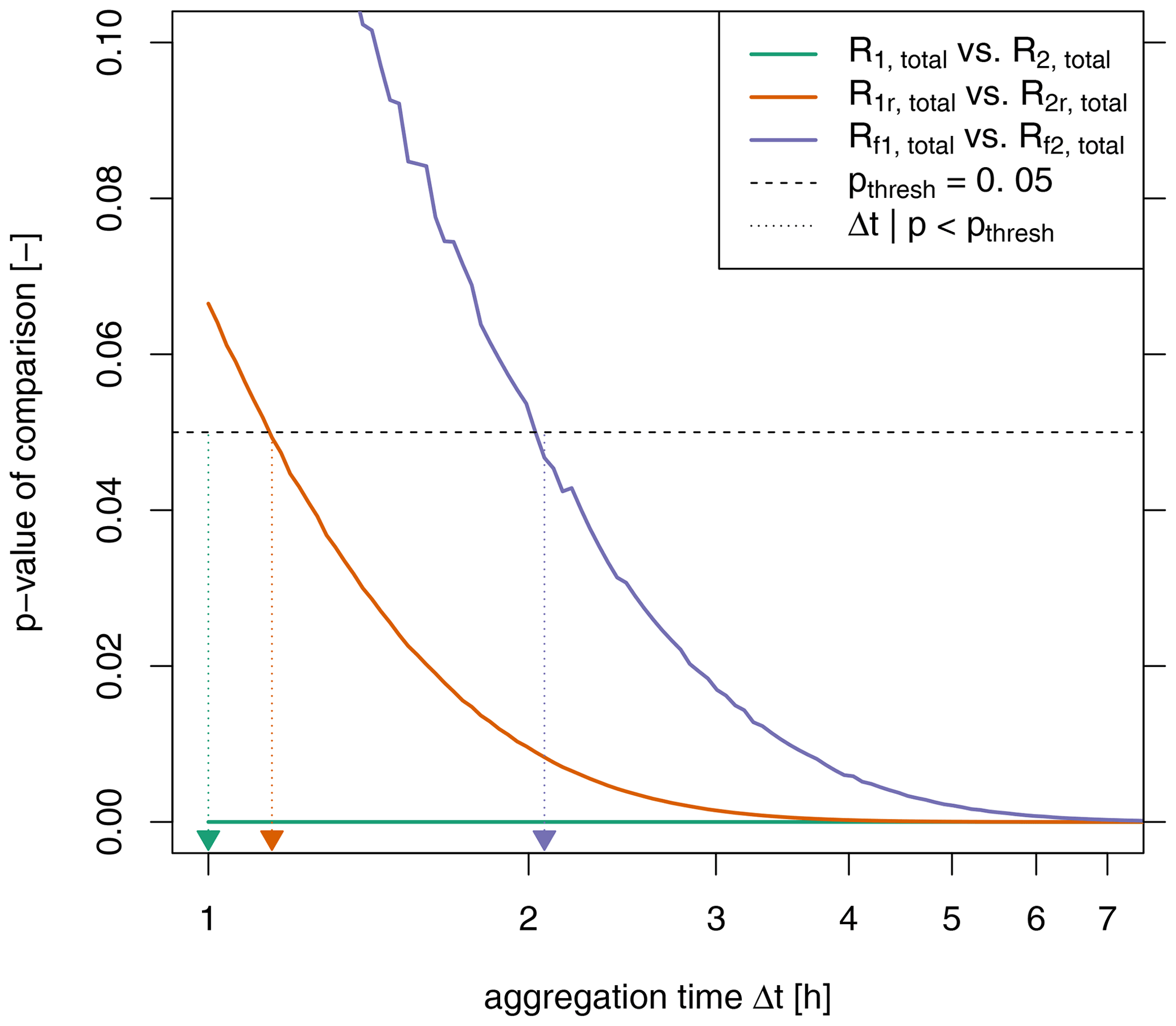
Figure 8 The p values for discriminating pairs of measured count rates ($R_{\mathrm{1},\mathrm{total}}=\mathrm{2100}$ counts h⁻¹, $R_{\mathrm{2},\mathrm{total}}=\mathrm{2520}$ counts h⁻¹, “favourable” scenario, moderate contrast ΔR=0.2). The vertical arrows indicate the minimum required aggregation time $\mathrm{\Delta }{t}_{\min }^{\mathrm{disting}}$ to statistically distinguish two rates at p=0.05.

In the context of distinguishing the two count rates, Fig. 8 shows that the p value for comparing two count rates decreases with increasing aggregation time. As one would expect, a statistically significant difference between two rates is more discernible with longer aggregation times. For the directly measured rates R_1,total and R_2,total, this distinction is possible even for the lowest aggregation times, while it takes longer for the reconstructed rates R_1r,total and R_2r,total. (Somewhat surprisingly, distinguishing between R_f1,total and R_f2,total is apparently even harder. The reconstruction of these rates using Eq. 14 evidently increases their signal-to-noise ratio.) How much aggregation time do we need to distinguish two count rates statistically? We choose the time $\mathrm{\Delta }{t}_{\min }^{\mathrm{05}}$ as an indicator for the time beyond which the difference between two rates R_1r and R_2r is significant at the 5 % level (brown arrow in Fig. 8).

So while an aggregation time of at least $\mathrm{\Delta }{t}_{\min }^{\mathrm{determ}}$ is needed to pinpoint one reconstructed value, we require $\mathrm{\Delta }{t}_{\min }^{\mathrm{05}}$ to distinguish two rates. These two objectives are different, and we will show that both indicators differ accordingly.

3.2.1 A. What temporal resolution can be obtained?

Figure 9 confirms that for higher count rates R₁ and R₂, less time is required to obtain a robust value from the directional measurements, i.e. confining the CI to less than 5 % of the actual value. The respective contrast between R₁ and R₂ is of relatively small effect for higher count rates but makes a difference for lower ones. For these, somewhat counterintuitively, a higher contrast requires longer aggregation times. This may be explained by the fact that these higher count rates are associated with larger absolute errors. When mixed with the weaker signal (see Eq. 14), they deteriorate its robust reconstruction. Consequently, a higher contrast in the rates aggravates the reconstruction of the lower one.

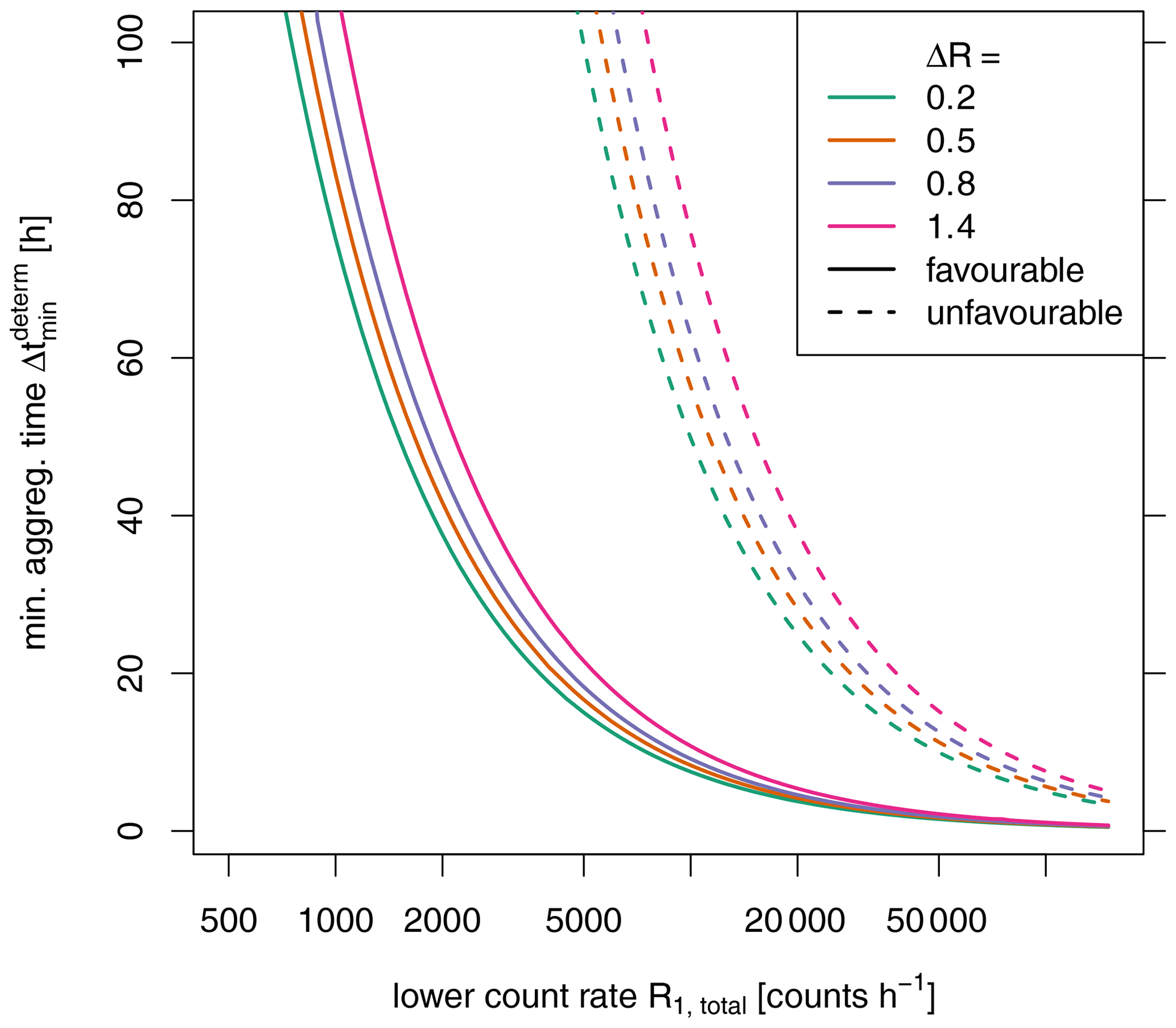
Figure 9 Minimum aggregation time $\mathrm{\Delta }{t}_{\min }^{\mathrm{determ}}$ required to obtain the reconstructed count rate R_1r from the two directional measurements with a CI smaller than 5 % of the actual value.

Figure 10 Minimum aggregation time $\mathrm{\Delta }{t}_{\min }^{\mathrm{disting}}$ required to statistically separate the reconstructed count rates R_1r and R_2r from the two directional measurements with p value < 0.05.

Conversely, Fig. 10 demonstrates that the statistical difference between R_1r and R_2r is easier to detect with a higher contrast between the two rates. This phenomenon effectively equates to the dilemma that the contrast in the count rates has the opposite effect, depending on whether we look at the precise determination of R_1r (benefits from low contrasts) or the statistical distinction between the two rates R_1r and R_2r (benefits from high contrasts). This distinction is apparently much more feasible within reasonable aggregation times: in the “favourable” scenario, hourly resolution can be achieved from count rates of above approximately 3000 counts h⁻¹ even for low contrasts. The “unfavourable” scenario increases the aggregation times by about a factor of 7.

For our example case, we can conclude that the precise determination of the count rates is hardly feasible even for the “favourable” scenario. Aggregation times exceeding at least 36 h are beyond the typical requirements in applications. Aggregation times of 24 h and less can only be achieved with count rates of more than 3100 or 20 700 counts h⁻¹ for the “favourable” or “unfavourable” scenario, respectively. Distinguishing the rates in the two half-planes, however, could be possible for aggregation times on the order of hours with even higher potential for stronger contrasts.

3.2.2 B. What spatial contrast in the count rates can be resolved?

Figure 11 again illustrates the phenomenon mentioned in the previous section: with higher contrast in the signal, estimating the weaker signal with the required precision gets more difficult (i.e. requires longer aggregation times or higher count rates). For reproducing values with high contrast (ΔR=1.4) in daily resolution, count rates R₁>4000 counts h⁻¹ are required for the “favourable” scenario. For the “unfavourable” scenario, R₁ must be larger than 40 000 counts h⁻¹ for this purpose.

Figure 11 Maximum possible contrast ΔR₂ in reconstructing the count rates R_1r from the two directional measurements with a CI smaller than 5 % of the true value.

Conversely, higher contrasts allow the statistical distinction of the two reconstructed rates also for lower count rates and aggregation times (see Fig. 12). According to the “unfavourable” scenario, even relatively low contrasts (ΔR=0.2) can be detected with the lowest considered count rates, if aggregation times are slightly higher than 24 h.

For our example case, we have already shown that the determination of the count rates is hardly feasible even for the “favourable” scenario. However, with aggregation times of 24 h, distinguishing rates with contrasts lower as 0.2 could be possible even for the “unfavourable” scenario.

Figure 12 Minimum contrast ΔR₂ required to statistically separate the reconstructed count rates R_1r and R_2r from the two directional measurements with p value < 0.05.

3.2.3 C. What count rates are required to yield robust estimates?

Figure 13 again stresses the need of high count rates to reconstruct the target count rates with the chosen precision. Specifically, to compute those rates in the “favourable” scenario at the daily resolution, the minimum count rate must be well above 3000 counts h⁻¹ for contrasts lower than 0.2. For the “unfavourable” scenario, this value increases to over 20 800 counts h⁻¹. As noted before, higher contrasts require even higher count rates (i.e. > 4500$/$31 000 counts h⁻¹ for the cases above) or longer aggregation times, which may exceed those required for practical applications (see Sect. 2.2.6, last paragraph).

Figure 13 Maximum possible contrast ΔR₂ to allow the reconstruction of the count rate R_1r from the two directional measurements with a CI smaller than 5 % of the true value with the aggregation time Δt.

Figure 14 Minimum contrast ΔR required to statistically separate the count rates R_1r and R_2r reconstructed from the two directional measurements with a p value < 0.05.

Concerning the statistical discernibility of R_1r and R_2r, Fig. 14 suggests that already low count rates allow the two reconstructed count rates to be distinguished. For the “unfavourable” scenario at the aggregation interval of 1 h, count rates of at least 15 600 counts h⁻¹ already allow resolving contrasts as low as 0.2. For the higher contrasts (ΔR=1.4), count rates of roughly 490 counts h⁻¹ would suffice.

Thus, for our example case, we would require at least 3100 counts h⁻¹ to successfully reconstruct both rates at 24 h resolution. The current count rate of 2100 counts h⁻¹ calls for aggregation times of at least 36 h. Merely distinguishing the rates R_1r and R_2r is possible with the given count rate at 1 h aggregation time.

3.3 Limitations and outlook

3.3.1 Assumptions made in the modelling and choice of parameters

This analysis is based on the geometries of a specific directional detector prototype. This prototype was designed with pragmatic considerations. So far, we have just been able to operate the prototype in a setting with sufficiently high contrast to practically indicate discrimination of count rates could be successful. Other designs (e.g. larger vertical planar shielding blocking off one half-space) may provide superior characteristics, namely η, which could be assessed by further neutron simulations.

The presented computations assume constant neutron flux rates. Evidently, this assumption is less realistic with increasing aggregation times: on the one hand, incoming neutron flux is subject to variation, though usually moderate; on the other hand, changes in the hydrogen pool within the footprint, namely due to hydrological processes, will add more variability to the signal, effectively increasing its error and aggravating the determination and discrimination of count rates.

The directional contributions obtained from the numerical neutron simulations apply to a setting with selected values for fixed hydrogen inventories. Increasing this inventory would decrease the sensor footprint. As the angular specificity decreases with distance to the sensor, we might expect somewhat improved directional contributions. However, in practice, an increased hydrogen inventory (i.e. from soil moisture and biomass) will usually also incur higher air humidity (deteriorating angular specificity) and reduced count rates, which counteract this effect. This is similar to the adverse effect of road-construction material on roving CRNS measurements (Schrön et al., 2018a). In-depth neutron simulations need to be used to clarify this issue.

Likewise, our setup also assumed spatially homogeneous hydrogen pools. Deviations from this assumptions, especially close to the sensor, will have a pronounced effect on the recorded signal due to the high sensitivity of the sensor in the short range. These effects will be detrimental to the reconstruction of representative count rates for the half-planes, unless the interpretation is restricted to this very proximity of the sensor.

With disparate flux rates R₁ and R₂ two additional concurrent effects will occur: if R₁ increases (e.g. less moisture in A₁), we would also expect more A₂ neutrons to be scattered back to the detector from A₁, because thermalization is reduced there. This deteriorates the directional contribution η for the reconstruction of R_r1 as we are getting more neutrons from the “wrong” direction. Conversely, the increased R₁ will tend to be more directional when coming from the area of less hydrogen (i.e. less scatter), in turn increasing the directional contribution for R_r1. Further neutron simulations are required to clarify which of these effects dominate and if they would notably influence η.

In our calculations, for the “favourable”/“unfavourable” scenario, we use fixed values for the fraction of “bycatch” count (ϵ) at 10 %/30 %. This assumption implies that these adjacent energy levels (thermal and fast neutrons) show a similar sensitivity to hydrogen. In reality, this sensitivity is considerably smaller and different but has been exploited in some studies (e.g. Baatz et al., 2015; Tian et al., 2016), effectively reducing uncertainties by increasing the rate of usable counts R_epi. However, measuring with only single moderated detectors does not allow for such a separation of the signal in terms of energy levels. Instead, the actual value of ϵ, being a function of hydrogen pools and chosen energy cutoff thresholds, poses another considerable source of uncertainty, which we neglect completely in this study by assuming a fixed value. A similar effect can be expected for the fraction of non-albedo neutrons γ: its range was considered in the scenarios; however, its actual functional dependency on the hydrogen inventory ignored in the analysis.

3.3.2 Implications for practical application of a directional sensor

Figure 3 suggests a setup of two independent detectors facing opposite directions. In this case, an imperfect calibration of their sensitivity can constitute another substantial device-specific error source, further aggravating the separation of the signals. Alternatively, a single sensor with temporally varying orientation (i.e. as presented in Sect. 1.2) could be used. While this eliminates the issue of imperfect calibration, it implies that all the computed aggregation times must be doubled, as the single sensor can cover each direction only half of the time.

The directional contribution η depends on the transport characteristics of the neutrons from the measured object to the sensor and the properties of the shielding. The former is governed by the surrounding medium (i.e. air pressure and humidity) and is beyond control in monitoring situations. The shielding, however, can be modified without theoretical limitations. Although obtaining a narrow FOV is still unfeasible because of the above-mentioned transport characteristics, hemispherical blocking could be increased to a large extent. It is constrained, however, by practical issues such as size, weight and price. Directional shielding larger than a few metres would hardly be practicable (transport, visual impact, wind stress); extending the shielding below the soil surface is certainly unfeasible, and a freely rotating setup poses even stronger limits. On the other hand, a concomitant use of two sensors could potentially use the same shielding. An enlarged version of the shielding would presumably also have higher directional contribution. The presented methodology could help to find reasonable compromises.

In the choice of example values, we also included some count rates obtained with setups of roving CRNS. These setups consist of a larger number of counting tubes. Consequently, they are considerably bulkier and could not be equipped with a shielding in the described dimensions, unless advances in sensor technology provide significantly smaller detectors. Even if such a shielding could be scaled up, the resulting weight would pose a severe challenge for realizing a practicable rotating sensor platform, thus calling for two complementary, non-rotating sensors instead, as mentioned above.

As a more angle-specific option for the shielding, micro-channel plates have shown favourable directional characteristics (Tremsin et al., 2005). However, their limitation to thermal neutrons, considerable costs and the remaining problem of non-geometric transport make them unfeasible for CRNS.

Materials with low hydrogen content and a high scattering-to-absorption ratio with respect to the nuclear cross sections, for example, graphite or quartz, can be used as reflectors towards the inside for directions to be blocked. Such reflectors can be used either on the insides or outsides of the moderator or in “shark” geometry between HDPE plates.

3.3.3 Further open questions for follow-up studies

We presented examples for a field of view of 180^∘. While smaller angles would be desirable for higher spatial resolution, such signals from smaller angles will be more difficult to resolve, due to the reduction of the count rates (smaller β). Although the above-mentioned methodology remains the same, the matrices A and B are no longer symmetric.

This study exclusively considered count rates as the target observation variable. However, for application, count rates are merely a proxy which need to be converted to the actual quantity of interest, namely soil moisture, snow or biomass. The relationships used in such conversion (e.g. Desilets et al., 2010) are not linear; instead, they saturate with increasing hydrogen pools and low count rates. This translates to an increased sensitivity of the target variable (e.g. soil moisture) for these low rates. This behaviour, therefore, amplifies the characteristics demonstrated in this study: considerably poorer applicability of directional CRNS measurements for lower count rates. Combining the presented approach with the one of Jakobi et al. (2020) would allow the direct quantification of uncertainty for the target variable.

4 Conclusions

This study combined neutron simulations with an analytical assessment of the directional specificity of epithermal neutrons and the potential for directional measurements in environmental monitoring.

The neutron simulations revealed the relatively low correspondence of incidence angle and angle to origin of the neutrons arriving at a CRNS detector. This is a direct effect of the non-geometrical (i.e. not direct) path of the neutrons, being subject to multiple collisions. Consequently, the correlation of these angles gets lower with increasing distance of the origin (i.e. the location of its conversion to epithermal). Thus, blocking certain incidence angles of a sensor only yields a limited angular specificity: for the investigated geometries of a directional shielding as a half-open rectangular box, the directional contribution was in the range of 60 % to 80 % for a target field of view of 180^∘. Moreover, this additional angular shielding reduced the overall count rates to about 30 %–40 %. This fundamental limitation is inherent to measuring neutrons under environmental conditions and cannot be alleviated by detector design and influenced only marginally by design of the shielding.

Based on these findings, the subsequent analytical analysis focused on the feasibility of determining and statistically distinguishing the count rates from two adjacent half-spaces by reconstruction from measurements of directional sensors. While the former benefits from a low contrast in count rates, the latter is aggravated by it. Both aspects profit from high count rates and longer aggregation intervals.

With the analysed setup and reasonable count rates, the accurate reconstruction of the two count rates is hardly feasible with less than 24 h of aggregation time, given detectors with conventional sensitivity. Thus, it seems to be of little value in environments where variability needs to be resolved at this timescale. While a substantial increase in detector sensitivity might address this issue, such an increase typically comes with higher costs and much larger detector sizes and hence an unfavourable increase in the dimensions of the required shielding.

The mere distinction of two rates, however, is more feasible and, even for moderate count rates and contrasts, perceivable at a resolution of a few hours. The effort of directional measurements for the mere purpose of distinction might appear somewhat incommensurate. Yet, the gain in information might be very relevant from a hydrological point of view, e.g. at the borders between grassland and forest which might experience a reversal of horizontal soil moisture gradients in periods of drying.

Progress in detector technology and optimizing the shielding towards wider FOVs but more specificity could alleviate some of the restrictions and make directional measurements a useful tool for tailored use of CRNS.

Appendix A: Symbols used in the text

Symbol	Explanation
A	matrix holding coefficients for mixing of albedo neutrons
B	matrix holding coefficients for mixing of all neutrons
β	count rate reduction factor due to shielding
ΔR	relative difference in the count rates R1 and R2
Δt	aggregation interval
ϵ	fraction of non-epithermal neutrons
η	directional contribution of shielding
γ	fraction of albedo neutrons in epithermal neutrons
J	matrix of ones
N	number of counted neutrons
pthresh	threshold p value
R	count rate
σ	error expressed as standard deviation
θ	volumetric soil moisture
Sub-/superscripts
!	non-…
05	concerning statistical distinction of rates
albedo	albedo neutrons, having interacted with hydrogen pools
determ	concerning determination of rates
dir	directional
epi	epithermal
f	shielded, i.e. directional detector facing towards a half-plane
!D	no shield, omnidirectional unshielded detector
r	reconstructed from directional measurement
D	shielded, i.e. directional detector
total	overall counts