the Creative Commons Attribution 4.0 License.
the Creative Commons Attribution 4.0 License.
 | 14 Apr 2023
Development of an expendable current profiler based on modulation and demodulation
Keyu Zhou
Guangyuan Chen
Zucan Lin
Yunliang Liu
Pengyu Li
We designed a low-cost expandable current profiler (XCP) including software and hardware. An XCP is an observation instrument that rapidly measures currents based on the principle that currents cut the geomagnetic field to induce electric fields. The cost of an XCP must be reduced because it is a single-use device. The digitization of the previously developed XCP is carried out underwater, which requires the probe to contain not only analogue circuits for acquiring signals but also digital circuits and digital chips, which are relatively expensive. In this study, an XCP was developed that adopts signal modulation and demodulation to transmit analogue signals on an enamelled wire, and the signal digitization occurs above the surface of the water. The cost of the instrument was effectively reduced by half while maintaining its ability to measure parameters such as sea current and temperature in real time. After comparison with data processed from laboratory tests, the acquisition circuit showed an accuracy within 0.1 % and the XCP analogue circuit developed for the overall system was stable and reliable. The system exhibited an acquisition accuracy higher than 50 nV for 16 Hz, and the quality of the acquired signal satisfied the requirements for an XCP instrument.
- Article
(4967 KB) - Full-text XML
- BibTeX
- EndNote


The expendable current profiler (XCP) is a single-use instrument that rapidly measures currents, mainly the velocity and flow direction of seawater, based on the principle that currents cut the geomagnetic field, inducing electromagnetic fields (S. Liu et al., 2017). The commonly used instrumentation methods for the measurement of ocean currents can be classified into floating, electromagnetic, mechanical, acoustic, and other (Peltier et al., 2013; Simpson, 2002; Jenkins and Bye, 2006; Le Menn and Morvan, 2020). The XCP is an electromagnetic current meter that produces rapid measurements using geomagnetism and uses a non-stop and non-recovery mode of operation, offering the advantages of a short detection period, instantaneous data acquisition, wider detection range, and various deployment forms (Niiler et al., 1991; Zhang et al., 2011; Hibiya et al., 2006; Jichang et al., 2009). Because the XCP is a single-use device and would not be recycled, it is important to reduce its cost.
Sanford et al. (1982) proposed a basic formula for the calculation of the electromagnetic field induced by seawater motion in 1971 based on Faraday's law of electromagnetic induction (Dunlap et al., 1981; Sanford et al., 1982). They then developed the prototype of the XCP in 1978 and conducted joint sea trials with the company Sippican, yielding preliminary test results (Dunlap et al., 1981; Sanford et al., 1982). At present, the core detection technology remains owned by the American and Japanese companies Sippican and Tsurumi-Seiki, respectively, and is embargoed in some countries (S. Liu et al., 2017; Szuts, 2012). In addition, the instruments of the companies have not been enhanced or improved since 2005. More recently, some Chinese universities and research institutes have started to research and develop XCPs. The authors successfully developed an XCP for digitization underwater (S. H. Liu et al., 2017), whereby the acquired analogue signal is digitized and then transmitted through a double-strand enamelled wire with an outer diameter of 0.1 mm. Testing showed that the method can transmit over more than 1000 m at a transmission band rate of 4800 bps (bits per second) (S. H. Liu et al., 2017; Zhang et al., 2013; Li et al., 2017, 2018; S. Liu et al., 2017). Digitization underwater requires the probe to contain not only analogue circuits for acquiring signals but also digital circuits and chips, such as the master control chip and related power conversion modules. Furthermore, the buoy board at the surface of the water that forwards and releases the probe uses master control chips, which are relatively expensive. Therefore, the total cost of the XCP is relatively high, which is not suitable for mass production.
Based on this, we have developed an XCP that adopts signal modulation and demodulation to transmit analogue signals on an enamelled wire and performs digitization above the surface of the water. Moreover, the digital circuitry inside the underwater probe was removed from our design. Because the XCP measured the induced electric field generated by the current cutting the geomagnetic field, which is a considerably small signal at a nanovolt level, if accurate current information needs to be measured, certain requirements must be satisfied for the accuracy and stability of the instrument. The measurement adopts the method of measuring frequency, which needs to generate frequency signals and to simultaneously compare and measure the frequencies and phases of multiple signals, including numerous calculations. Therefore, the measurement requires significant resources; therefore, the main control chip should have certain resources and performance, which determines the price of the chip. In this design, the added modulation and demodulation component of the XCP is mainly composed of amplifiers, counters, resistors, and capacitors, and the cost of this chip is low. In addition, we replaced and optimized some other components of the entire system and selected the scheme with the best cost performance. Therefore, the cost of the instrument is effectively reduced while retaining the measurement functionality in real time on parameters such as sea current and temperature. This should pave the way for widespread adoption and mass production. We also carried out the laboratory analogue circuit test. Through the data processing and comparison of the laboratory test, we found that the accuracy of the acquisition circuit was within 0.1 %. The XCP analogue circuit developed by the overall system was stable and reliable. For the 16 Hz signal acquisition, the accuracy was better than 50 nV, and the quality of the acquisition signal met the requirements of the XCP instrument. In addition, we have constructed a laboratory flume simulation environment, tested the biogenic electric field in the simulated sea environment, and compared the results with those acquired by the previously developed XCP, which were found to be highly consistent. In addition, we simulated the real ocean current in the hydrodynamic large-scale velocity environment developed by the North Sea Environment Monitoring Center of the State Oceanic Administration of China and compared it with the mature product Nortek Vectrino Profiler (acoustic Doppler velocimetry, ADV). The maximum velocity deviation was 0.0521 cm s−1, which meets the measurement accuracy requirements of the XCP.
The basic principle of the XCP was proposed by Sanford (1971, 1982) and Sanford et al. (1978) in the 20th century and subsequently analysed and studied by various researchers (Jenkins and Bye, 2006; Niiler et al., 1991; Zhang et al., 2017); therefore, further elaboration is not provided herein.
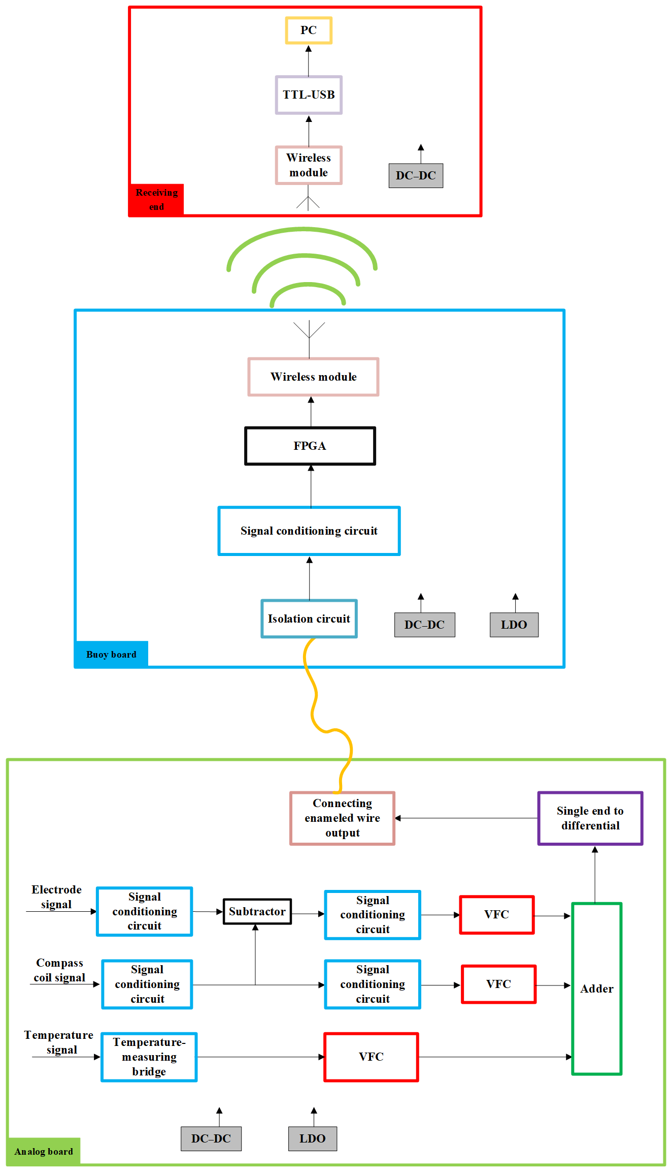
The usage procedure of the XCP developed in this study is similar to existing ones. Figure 1 shows the schematic of XCP operations. After the device is cast into the sea, the buoy board is automatically powered upon touching the seawater, and XCP probes are automatically released at regular intervals. The probes rotate and sink at a frequency of 16 Hz and would also automatically power up when launched into the seawater. While sinking, the electric field and temperature sensors collect data that are transmitted to the buoy board in the form of analogue signals through an enamelled wire. After the buoy board has demodulated the signals, they are digitized, and the processed data are sent to the host computer via a wireless module. The data are then analysed and processed by the host computer, and the waveform is displayed in real time.

The overall architecture of the instrument is shown in Fig. 2. The interior of the probe consists of three sensors and an analogue board. The buoy board consists of an analogue board, digital board, wireless transmitter board, and antenna. The receiver on the deck consists of a wireless module board and antenna. The analogue board and buoy board are connected by 1500 m of enamelled wire, which is used to transmit signals from underwater to the surface. For each part of the circuit board, we use lithium batteries for the power supply. Because each module requires different voltages, we use different power conversion modules (DC–DC) for voltage conversion. Simultaneously, to reduce power noise, we use a low dropout linear regulator (LDO). The LDO has the advantages of lower noise and lower static current. In Sect. 3, we separately introduce each part of the XCP.
3.1 Circuit design of underwater part
The analogue board contains a front-end electric field sensor, direction sensor, and temperature sensor. After the analogue signals acquired by the front-end sensors are conditioned, the three voltage signals are converted into three frequency signals with different intervals using voltage–frequency conversion (VFC), which are then superimposed and modulated into one signal for transmission.
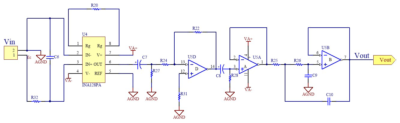
The electric field and compass coil signals are first amplified by the low-power precise instrumentation amplifier INA128 through the electrode and direction sensor and then sent to the voltage-to-frequency converter chip through a series of amplification and filtering. The INA128 is a general-purpose instrumentation amplifier with high accuracy and low power consumption developed by Texas Instruments and is commonly used in situations requiring high accuracy and circuit stability. The INA128, as an amplifier, is very easy to debug and operates in the temperature range of −40 to 85 ∘C, while maintaining low drift characteristics with a maximum temperature drift of only 0.5 µV ∘C−1 (INA128, 2022; Ren and Cheng, 2011), making it ideal for the undersea operations of the XCP. The schematic diagram of the coil channel acquisition circuit is shown in Fig. 3. With the final addition of a second-order controlled voltage source to the Butterworth low-pass filter circuit, the cut-off frequency is set to 16 Hz to filter out high-frequency noise.
The temperature signal is acquired through a temperature-sensitive resistor using a typical bridge circuit with high-precision voltage dividing resistors. After the temperature information is converted into a voltage signal, it enters the voltage-to-frequency converter chip that then outputs the frequency signal. The voltage-to-frequency conversion circuit modulates the three signals in different frequency bands using different resistor–capacitor parameters. The three frequency signals are processed by band-pass filters and then superimposed by an adder, modulating them into a frequency division multiplexed signal. This signal is inverted into a signal of the opposite phase but the same amplitude, and then it is connected with the original signal to the two ends of a double-enamelled wire, forming a pair of differential signals for transmission. The underwater probe section has one less digital board compared to the previously developed XCP (S. Liu et al., 2017), which reduces the cost by approximately half.
Since the acquired signal is extremely weak and of nano-voltage level, there are three grounds on the analogue board to reduce interference: analogue, power, and seawater. Connecting each ground with magnetic beads can effectively reduce interference. Figure 4 is the circuit schematic diagram of the switch part of the analogue board that is in contact with water. Power1 is an externally powered lithium battery, with one “key” pin connected to the seawater using the same material as the electrode and the other pin connected to the ground of the battery on the board. When the probe enters the seawater, the seawater becomes connected to the board ground, pulling the sixth pin of the CD4013 chip to a low level. This reverses the first-pin level, connects the metal-oxide-semiconductor (MOS) tube, and supplies the voltage of the lithium battery to the whole board. The water entry power method was tested for speed and stability and could be applied to other expendable instruments.
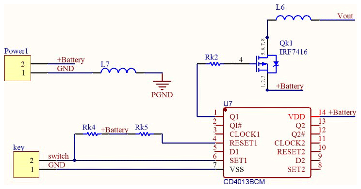
Figure 4Circuit schematic diagram of the switch part of the analogue board in contact with water.
3.2 Circuit design of the above-water part
The circuit board in the buoy is mainly composed of an analogue board, digital board, and wireless transmitter board, and the block diagram of the structure is shown in Fig. 5. The analogue board demodulates and conditions the modulated signal on the enamelled wire into a digital signal that can be recognized by the main control chip. First, the differential signal transmitted through the enamelled wire is isolated and amplified by a transformer. Second, the signal is amplified and converted into a single-ended signal by an adaptive amplifier, and the three frequency signals are separated and demodulated by a three-way sixth-order band-pass filter circuit. Lastly, the three frequency signals are multiplied separately for greater accuracy. The multiplied signals are further processed in the field-programmable gate array (FPGA) on the digital board.
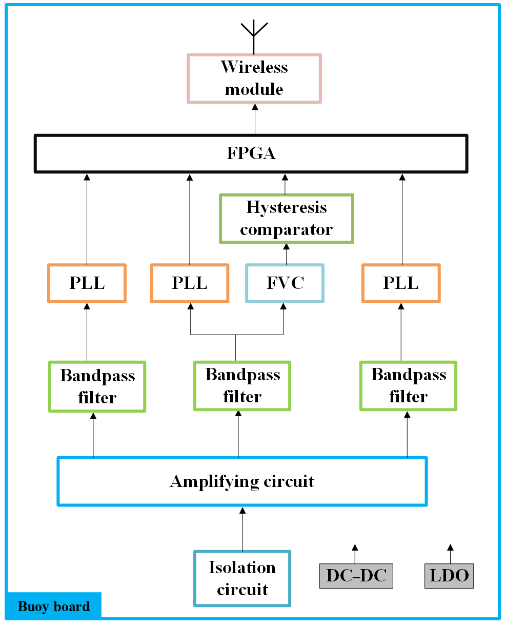
The frequency multiplication circuit adopts a typical CD4046 phase-locked loop (PLL) with a counter, as shown in Fig. 6. The binary counter CD4040 is used for frequency division, that is, the frequency of the output signal of the PLL voltage-controlled oscillator (VCO) is 2n times the frequency of the input signal. Because the maximum frequency division of counter CD4040 can be as high as 212=4096, the afore-described multiplication circuit is therefore capable of multiplying the input frequency by a maximum of 4096. To enhance the measurement accuracy of the XCP, the temperature and electrode coil signals are multiplied 256 and 32 times, respectively, according to the actual situation to achieve horizontal and vertical resolutions of 1 and 0.3 m s−1. Tests showed that the actual PLL frequency multiplication circuit is stable and reliable in operation. Figure 6 shows the schematic diagram of the frequency multiplication circuit. Figure 7a and b show the output waveforms of the multiplied frequencies at 32 and 256 times, respectively, when the 1 kHz signal is input into the PLL. Figure 7c shows the amplified waveform of the multiplied frequency at 256 times. The desired multiplication output can be obtained by varying the value of the division frequency of the counter. This PLL circuit can realize synchronous sampling and equal interval sampling well, as it improves the calculation accuracy, reduces the MCU computing time, and improves the real-time control performance (Murtianta et al., 2016; Zhihong et al., 2008).
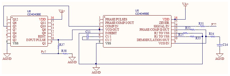
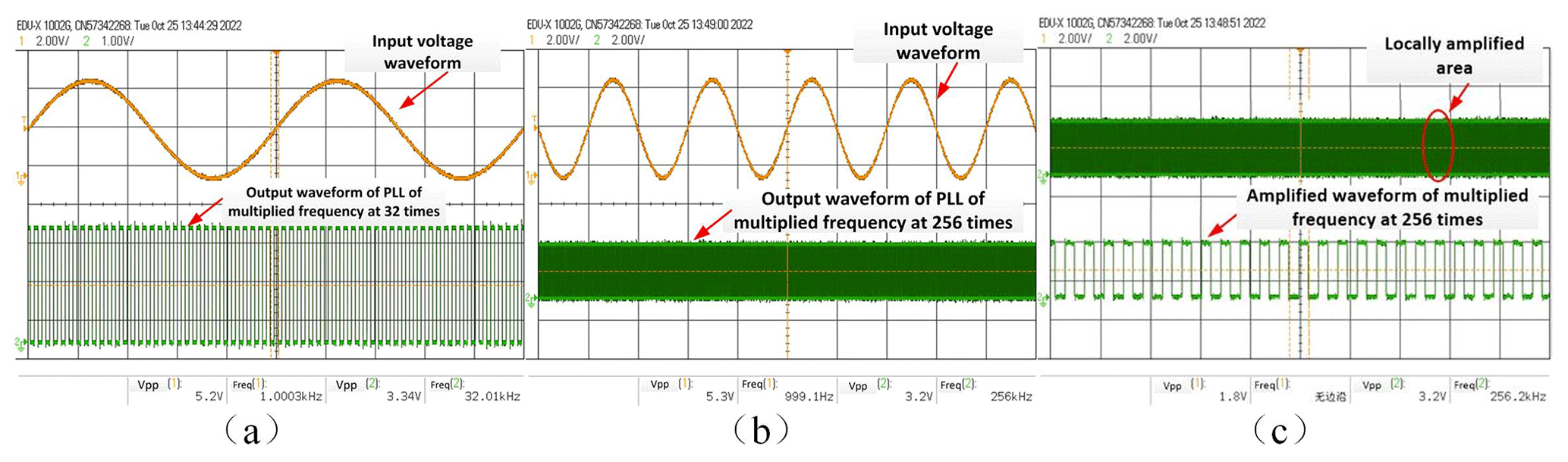
Figure 7The output waveform of a phase-locked loop of multiplied frequency at (a) 32 and (b) 256 times and (c) amplified waveform of multiplied frequency at 256 times. (© Keysight Technology EDUX1002G Digital Storage Oscilloscope).
The digital board includes the FPGA minimum system, power conversion module, water entry power module, probe releasing module, and more. The information output of the electric field, coil, temperature, and more from the main control chip after calculation, calibration, and other steps is sent to the deck unit through the wireless module.
The probe release section is controlled by a typical MOS switch circuit with a high-power 510 Ω chip resistor on the circuit board. The resistor is heated up by adding 5 V to both ends, thereby melting the resistor wire that controls the bottom cover of the probe, and after the wire is broken, the bottom cover comes off and the probe drops. The resistor heating time was tested to minimize battery power consumption, and it was found that 10 s was sufficient for the wire to fuse. Therefore, the MOS tube turns off after 10 s, and the resistor stops heating up.
The wireless data transmission module, which is the same as the one inside the buoy board, receives data at the deck unit end and connects to the PC via USB. The wireless SRWF-1028 module from Shanghai Sunray Technology Co., Ltd was used. This general-purpose transparent transmission module incurs low power consumption and has transmitting and receiving currents at approximately 350–500 and 32–38 mA, respectively. It can accommodate standard or non-standard user protocols, has excellent anti-interference capability, and has a long transmission distance with a handheld and line-of-sight distance of up to 2500 m. The baud rate is set to 9600 bps and the working frequency to 433 MHz.
3.3 Software design
Since higher-frequency signals are to be acquired, the digital master control chip of the lower part of the buoy board adopts the Cyclone series FPGA from the company Altera (S. Liu et al., 2017). The Nios II embedded processor control code, written in the C language, processes the transmitted signal data, transmits the data, times the probe release, and more. The software workflow diagram is shown in Fig. 8. Because the operation of the ship would interfere with wireless communication, after we release the buoy, it would have 180 s before releasing the probe, as shown in Fig. 8. Because the expendable instruments are operated in a non-stop manner, the ship would have moved a long distance within 180 s, and this would not affect the wireless data transmission. As mentioned in the previous section, our wireless transmission distance can reach 2500 m, and the ship cannot travel beyond 2500 m within 180 s. Therefore, the problem of hull interference with wireless communication is ingeniously solved.

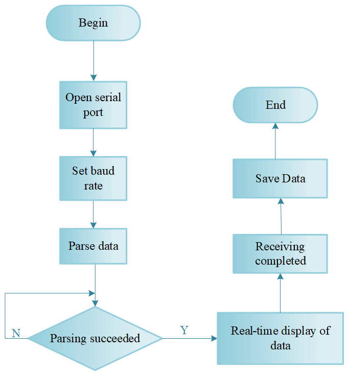
The upper computer software is developed in the C# language with Visual Studio 2022, and the functions include receiving data from the serial port, displaying waveform, exporting files, and so on. It has a user-friendly human–computer interaction interface and integrates the function of sea current flow rate processing by calling MATLAB code for calculation and drawing, allowing real-time processing, and displaying sea current information.
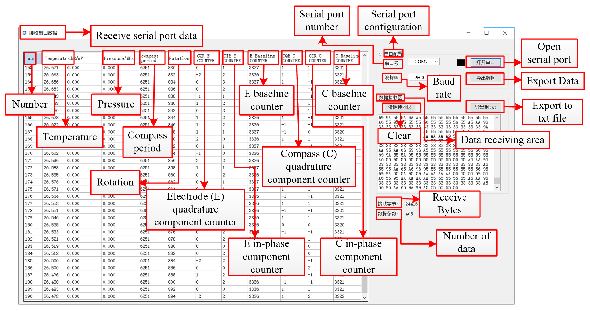
The workflow diagram of the upper computer is shown in Fig. 9, and the interface of the serial port receiving data is shown in Fig. 10.
The acquisition circuit was tested in our laboratory by simulating the entire system and comparing it with the results of the previously developed XCP.
4.1 Testing of acquisition circuit
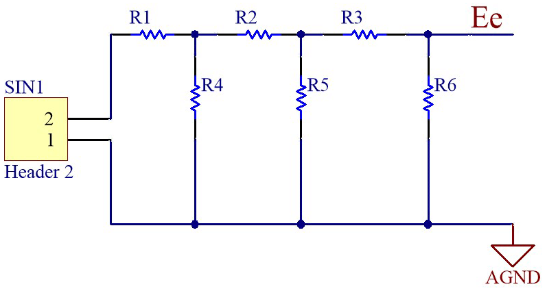
The accuracy of the acquisition circuit was tested. Ordinary signal generators are unable to produce nanovolt-level signals owing to the relatively small electrode and coil signals, and they are also susceptible to mixed industrial frequency interference when propagated through wires. Therefore, a resistive attenuation network was added to the acquisition circuit for accuracy testing, although none would be added for the actual measurement. The attenuation circuit is shown in Fig. 11, and its attenuation multiplier could be changed by varying the resistor value. The resistance thermal noise voltage is proportional to the resistance value, bandwidth, and square root of the temperature (K). Essentially, the resistance thermal noise is unavoidable. However, to minimize the noise caused by resistance, selecting resistors with large resistance values should be avoided.
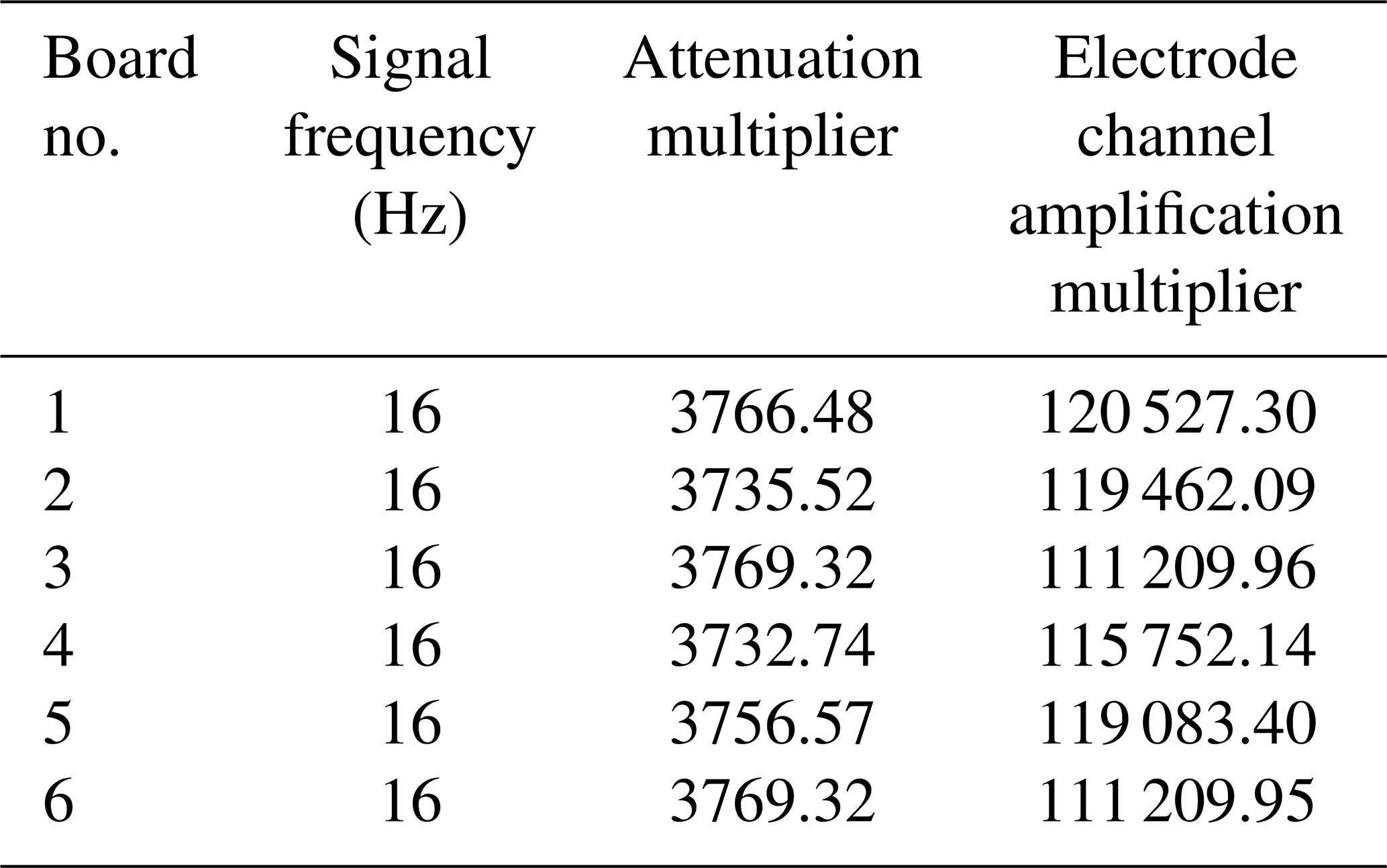
Because the values of resistance and capacitance would contain certain errors, to obtain accurate readings the accurate amplification of each analogue board must be measured; that is, the device must be calibrated. We use a lock-in amplifier to calibrate the analogue boards. The attenuation multiplier was set to approximately 3700 times, and a sinusoidal signal with a root mean square value of 0.4 mVrms (millivoltage root mean square) at 16 Hz was output using a lock-in amplifier. The peak value of the signal was approximately 50 nV after passing through the attenuation circuit; it then entered the electrode channel, and the output signal was measured by the lock-in amplifier after amplification. The information displayed by the lock-in amplifier was used to calculate the attenuation and amplification multipliers, and this method was used to calibrate each board to determine the exact multiplier of amplification. As the coil channel had a relatively small multiplier of amplification, it was connected directly to the lock-in amplifier without attenuation. We made six analogue boards (they were numbered from one to six) and then tested for their corresponding multipliers of amplification. The measured multipliers of the electrode channel and coil channel amplifications are shown in Tables 1 and 2, respectively. We used Excel to record and calculate the results and reserved two decimal places for the results. It is evident from the data in the table that although each circuit board is welded with the same components, the total amplification or attenuation times are relatively large, and small differences in the values of each resistance and capacitance in the circuit lead to large differences in the amplification or attenuation times of the whole circuit board. Therefore, the calibration of each circuit board is of great significance to the accuracy of the results. Figure 12 shows the final output waveform as seen with an oscilloscope for the coil channel of board no. 2, revealing a good signal quality with a peak-to-peak value of 3.06 V and an error accuracy that is within of the theoretical value. There are numerous works of research on weak signal processing circuits in China; however, most of them relate to the fields of exploration, medicine, and biology, and the acquired signals are mostly at the microvolt level (Levkov, 1988; Si et al., 2016; Lai et al., 2012; Dohnal, 2019; Lu et al., 2022). In contrast, an induced electric field produced by currents with a flow rate of 1–3 cm s−1 at midlatitudes was shown to have a signal of approximately 20–80 nV as measured by an electric field sensor with a spacing of 5 cm (Liu et al., 2011). The results of the experiments show that both the multipliers of the electrode and the coil meet the requirements for the acquisition of the multiplier of the signal.
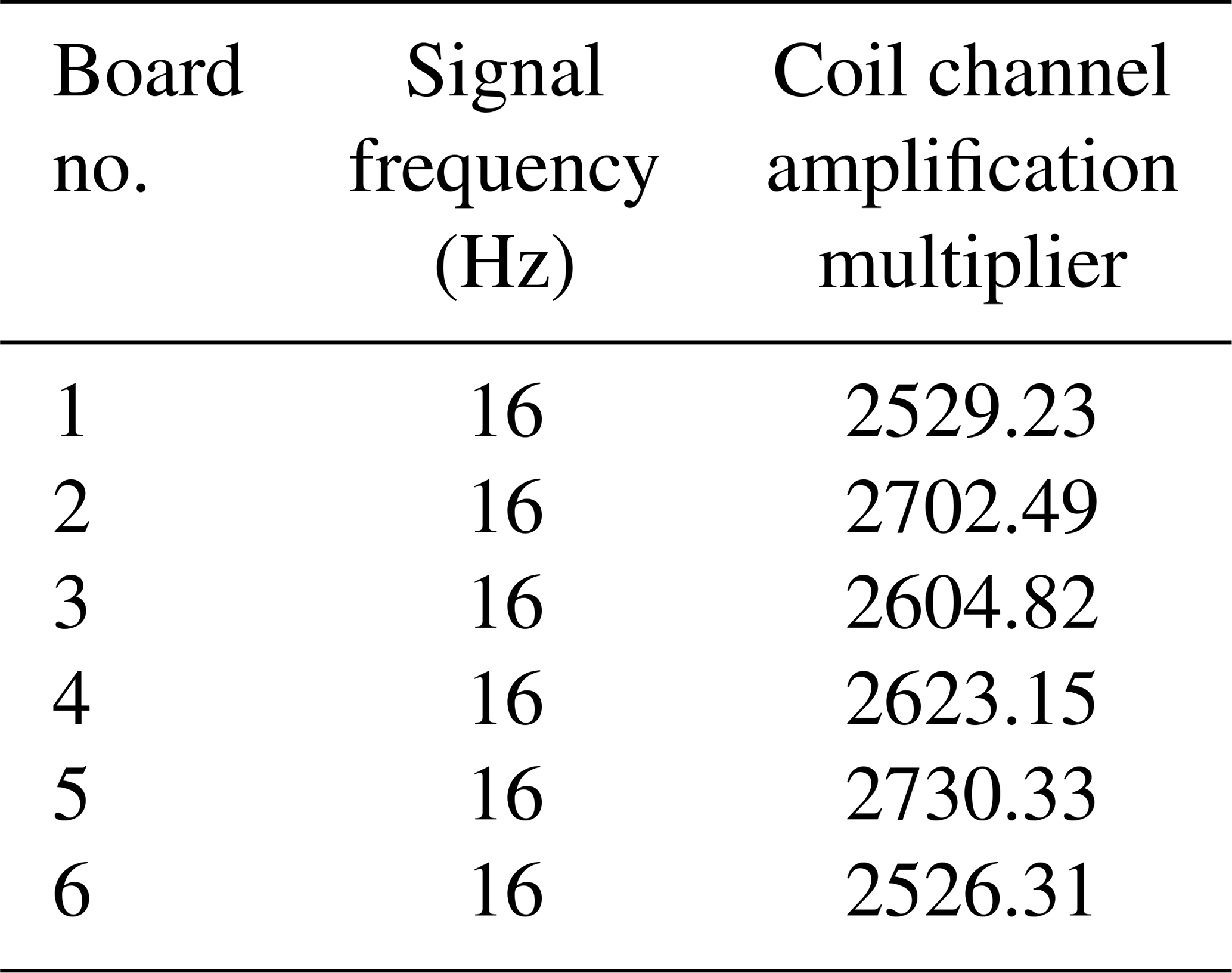
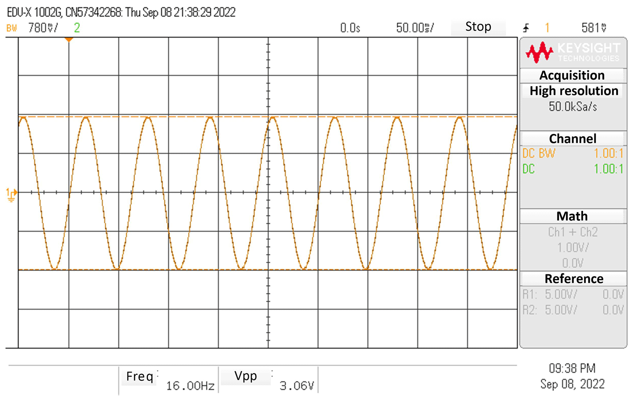
Figure 12The output waveform of the coil channel (© Keysight Technology EDUX1002G Digital Storage Oscilloscope).
4.2 Tests with added direct-current field inside and outside the laboratory
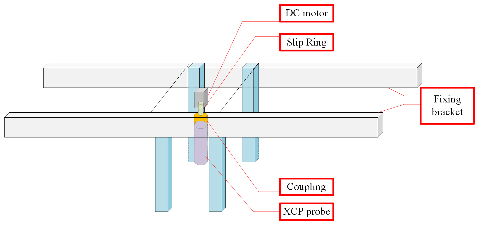
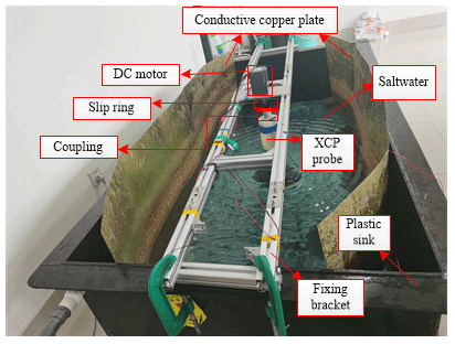
The laboratory test was carried out in a plastic tank with simulated seawater. In the test, because the XCP is used in the ocean, we need to use seawater for the test. Because it is not convenient to obtain real seawater, we use artificial seawater instead of natural seawater indoors. The conductivity of seawater is mainly related to salinity, and the average salinity of seawater is about 35 %. Therefore, to better simulate the conductivity of seawater in the experimental environment, tap water and sea salt are configured according to the salinity of seawater. By calculating the volume of tap water in the plastic tank, we determine the weight of sea salt required according to the average salinity of 35 % in seawater and the salinity in sea salt. The XCP probe is required to rotate with an angular velocity of approximately 16 Hz while dropping, so that both the compass and coil signals are modulated into an approximate single-frequency signal with a frequency of 16 Hz, according to the characteristics of the current electric field and compass coil signals. A rotating structure device was designed consisting of a small direct-current brushless motor, a holder to fix the motor, an XCP probe, a fixture to fix the XCP probe, a coupling, and a conductive slip ring. The structure of the device is shown in Fig. 13. The direct-current motor is controlled by the controller and can rotate at a speed of up to 16 Hz. The function of the conductive slip ring is to allow for the rotation of the lower wire of the signal transmission as the motor rotates while keeping the upper wire stable and stationary so that the signal transmission wire would not become tangled. The function of the coupling is to enable the XCP fixing structure to rotate coaxially by driving force from the motor shaft, which enables the XCP probe to rotate. We use a 1500 m long double-strand enamelled wire with an outer diameter of 0.1 mm for signal transmission, and the coupling is connected to the buoy end.
Copper plates were placed at both ends of the trough and direct current was added to both plates. By controlling the motor to rotate the XCP, the direct current was converted into alternating current, which was measured by the electrodes and transmitted inside the XCP for processing. The experimental setup is shown in Fig. 14.
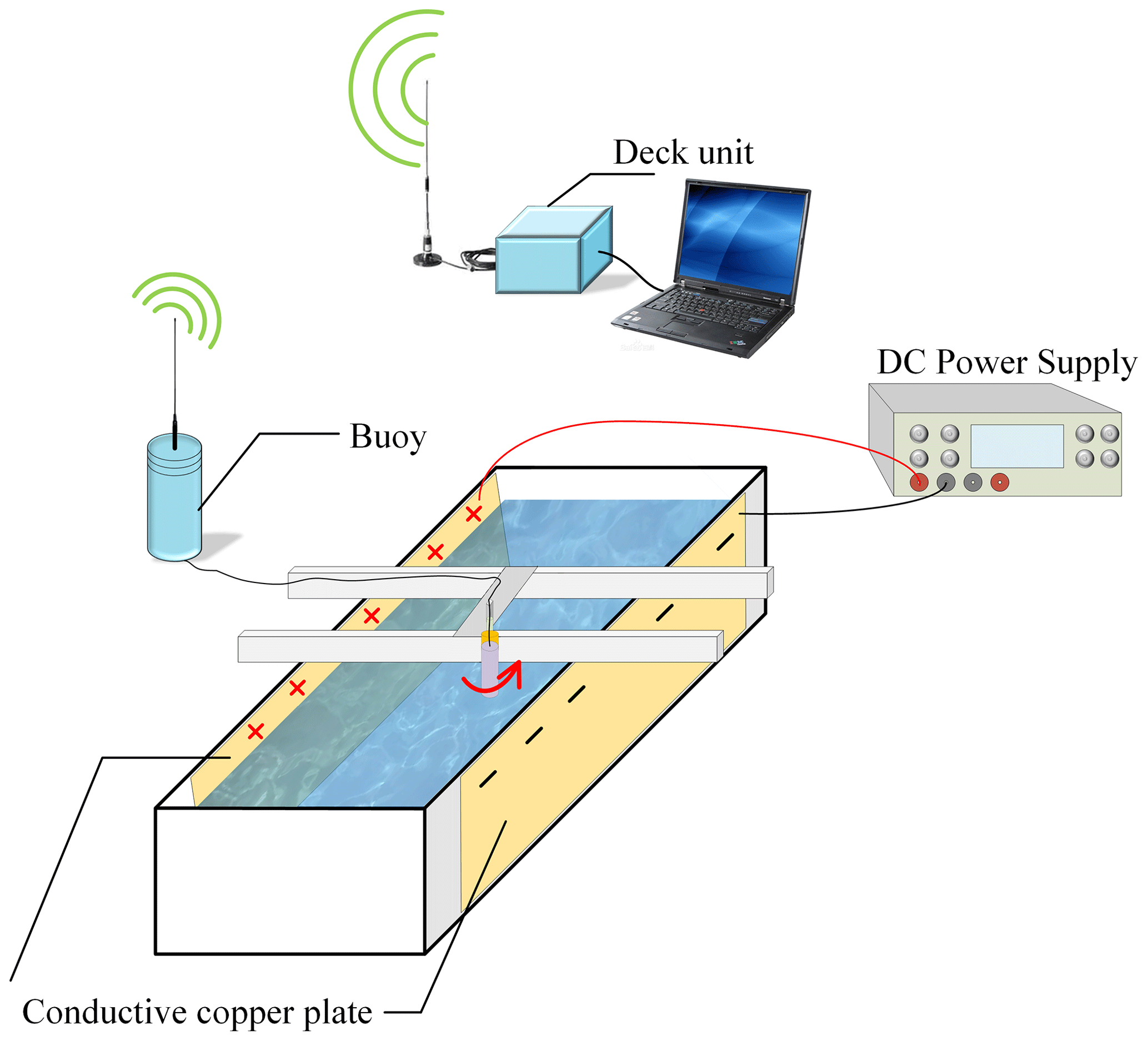
The magnitude of the voltage of the direct-current regulator source was altered, and the voltage data of the copper plates were measured with a digital multimeter. The data from the XCP probe were received and transmitted back to the host computer and then processed to calculate the peak-to-peak values of the measured electrode voltages. As the experiment was conducted in the laboratory, there was a substantial amount of noise compared to the marine environment. The ocean is comparable to a low-pass filter whereby all high-frequency noise from human sources would not interfere with the ocean electromagnetic signal, whereas a laboratory test environment may have noise interference, such as industrial frequencies. Therefore, a millivolt level signal was added to both ends of the copper plates so that the electrode measurements were set roughly to the microvolt level instead of the nanovolt level to reduce the interference from noise caused by human activity. We used the same test method to test two XCP probes. The experimental test photo is shown in Fig. 15.
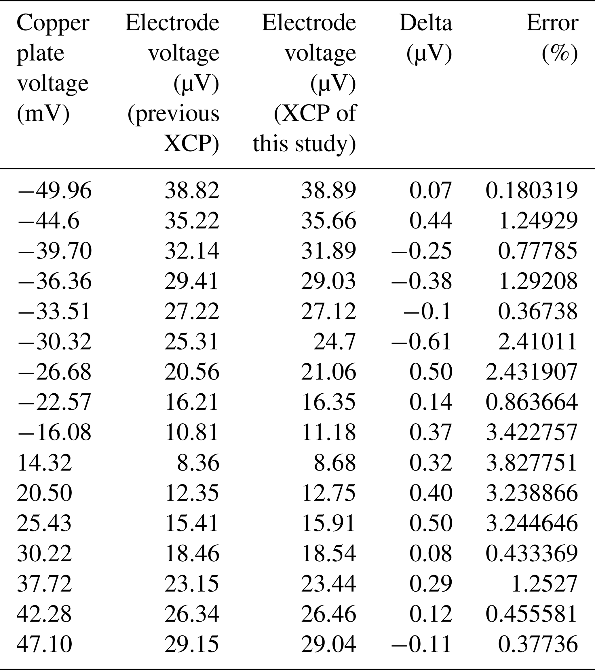
A comparison of the results of the two XCP probes is shown in Fig. 16. It can be observed that the measured voltages of the two probes were consistent with the trend of the copper plate supply voltage, and the results obtained by the two probes were largely the same when the copper plate supply voltage approximately ranged from ±5 to 54±70 mV. When the copper plate supply voltage ranged from ±5 to 54±70 mV, the difference between the peak-to-peak values of the electrodes measured by the two probes was the largest at the reverse supply voltage of 30.32 mV, which was 0.61 µV. When the copper plate voltage was less than 5 mV, the measurement results of both probes became unstable simultaneously and fluctuated in the approximate range of 2–5 µV, indicating that noise interference did exist in the laboratory environment. When the copper plate voltage was greater than 54 mV, the voltage measured by the XCP remained largely constant, indicating that the amplifier was fully saturated.
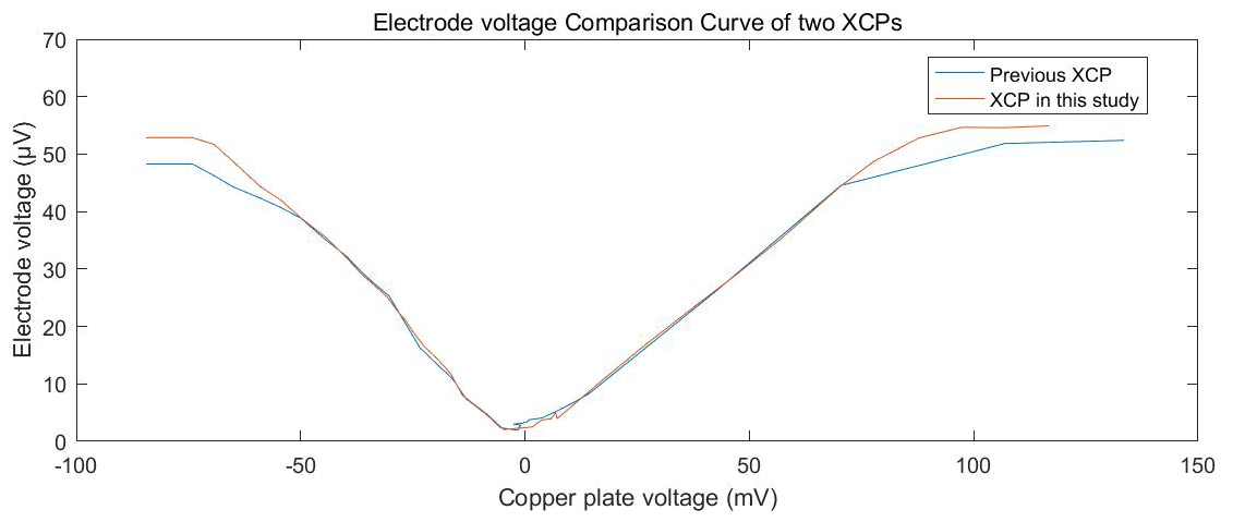
Based on the above analysis, we needed to eliminate the interference of indoor noise over the range of the results. Therefore, we selected the data in the middle of the copper plate power supply voltage between ±15 and ±50 mV, with the voltage remaining measured to two decimal places. We listed these voltages in Table 3 to display the data more accurately. The actual acquisition accuracy errors in the two probes are within 3.9 %, and the maximum error is 0.61 µV. We surmise that the error may be related to the inherent noise in the laboratory test environment. In addition, the operation of the motor could also have an impact on the accuracy. These interferences would not occur in the marine test because the ocean is far from polluting noise interferences such as alternating current found in the city environment. The XCP with which the comparison was made had undergone marine tests in a previous study and the results showed that this XCP worked with stability and accuracy (S. Liu et al., 2017); therefore, this result has a high reference value.
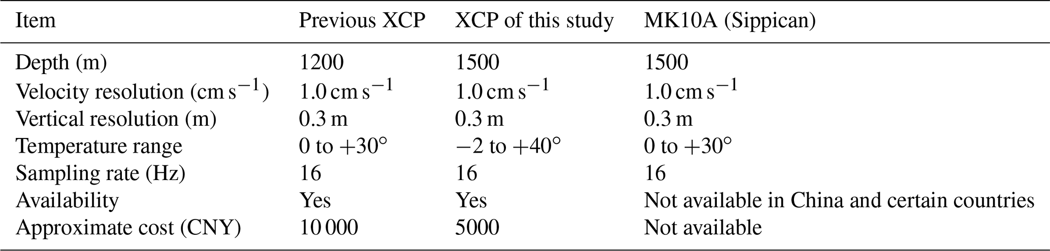
We also compared the XCP performance with the existing XCP performance. Table 4 lists representative performance indicators of this XCP and, for comparison, those of the previously developed XCP and the Sippican MK10A XCP (from lockheedmartin.com). It can be observed that we successfully reduced the cost on the premise of ensuring accuracy, which is of great significance for expendable instruments.
The temperature is related to the range of VFC. Because the XCP is used to measure current parameters in seawater, the mixture of ice and water has a temperature of 0 ∘C, and the temperature of the world's oceans generally varies between −2 and 30 ∘C. Therefore, we set the minimum threshold to −2 ∘C.
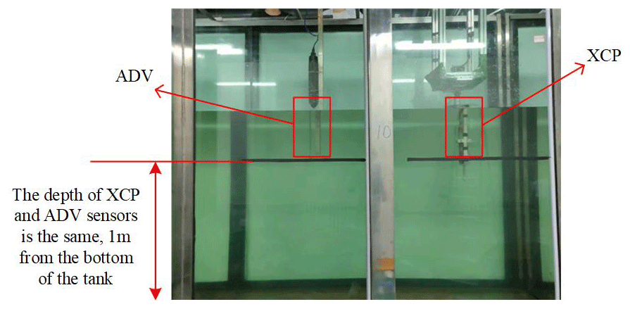
In addition, we compared it with mature products to better reflect the performance of the instrument. We carried out an XCP probe rotation simulation test under the hydrodynamic large-scale velocity environment at the Beihai Environmental Monitoring Center of the State Oceanic Administration of China. The Key Laboratory of Bohai Ecological Early Warning, Protection and Restoration of the centre has built a large hydrodynamic wave current simulation tank, covering an area of approximately 125 m2, with a length of 32.0 m, internal width of 0.8 m, internal depth of 2 m, and maximum working depth of 1.5 m. The working medium uses seawater. When the working water depth is 1.5 m, it can produce a uniform and stable flow field adjustable within 0.1 m s−1, which satisfies the requirements of this experiment. In this experiment, Nortek Vectrino Profiler Acoustic Doppler Velocimetry was used as the comparison equipment. The specific layout of the experimental equipment is shown in Fig. 17.
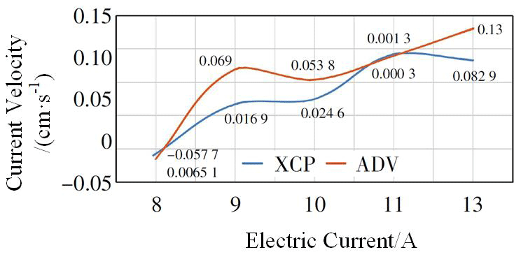
Under different current-generation gears of the flow rate tank (based on the working current level of the current generation generator: 8 A, 9 A, 10 A, 11 A, and 13 A), we performed the comparison test of the ADV and the XCP rotating flow rates. Owing to the limited accuracy of the flume, the principle of the two forms of test equipment is different, and the accuracy and error sources are different; therefore, some errors would be present. As shown in Fig. 18, the overall change trend of the velocity data curve collected by the ADV and the XCP is consistent; as the current increases, the measured flow rate increases. Moreover, the velocity value measured using the acoustic method is slightly higher than that using the electromagnetic method, which may be caused by the slight interference of the metal reinforcement framework of the tank and the current generator with the geomagnetic field, which does not exist in the actual marine application. The maximum velocity error occurs at the ninth speed position of the current generator, with a velocity deviation of 0.0521 cm s−1. For the XCP measurement accuracy of 1 cm s−1, the deviation is approximately 5.2 % of the total accuracy, which satisfies the XCP test requirements within the allowable range of test error.
In this study, we designed the hardware and software for a low-cost XCP. In addition, we built a test environment to test its accuracy and stability. The specific conclusions of this study are as follows:
-
We designed the analogue circuit of the signal processing part, including the water contact switch, delayed release switch, frequency multiplication circuit, signal conditioning, and more. These circuits could also be applied to other expendable instruments and instruments that need to obtain small signals.
-
We conducted circuit tests. Testing revealed that the accuracy of the XCP acquisition circuit is within 0.1 % and the XCP analogue circuit developed for the overall system is stable and reliable with an acquisition accuracy greater than 50 nV for a 16 Hz signal, which meets the quality requirements for acquired signals of XCP instruments. An experimental device for indoor XCP testing was introduced, and a passive source simulation experiment was carried out.
-
The data from the passive source simulation experiments were compared with those of the previously developed XCP that was validated with marine tests (S. Liu et al., 2017). The results of the two probes were found to be highly consistent with a maximum error of 0.61 µV, indicating that the XCP is stable and reliable.
-
Under the condition of large-scale hydrodynamic flow velocity developed by the North Sea Environment Monitoring Center of the State Oceanic Administration of China, we simulated the real ocean current and compared it with the mature product ADV. The maximum velocity deviation was 0.0521 cm s−1, which satisfies the measurement accuracy requirements of the XCP.
-
The XCP developed in this study moved the processing circuit to above the surface of the water, reducing the use of underwater components and chips and effectively reducing costs. It is estimated that the cost of the XCP probe is reduced by half.
However, there still remain some areas wherein we can further optimize and improve. For example, our accuracy remains the same as before, and the measurement parameters have not increased. In the future, we will improve the accuracy, study the effect of increasing the measurement parameters and measurement distance, and improve the data transmission mode. In addition, we aim to achieve mass production as soon as possible.
There are no publicly available data for this study.
Conceptualization: QZ and GC; methodology: QZ and KZ; software: ZL and KZ; validation: KZ, ZL, PL, and YL; formal analysis: KZ; investigation: KZ; resources: QZ; data curation: KZ; writing – original draft preparation: KZ; writing – review and editing: KZ; visualization: KZ; supervision: QZ; project administration: QZ and GC; funding acquisition: QZ and GC. All authors have read and agreed to the published version of the paper.
The contact author has declared that none of the authors has any competing interests.
Publisher's note: Copernicus Publications remains neutral with regard to jurisdictional claims in published maps and institutional affiliations.
We have been supported by the China University of Geosciences (Beijing), Shandong University of Science and Technology and Beihai Environmental Monitoring Center of the State Oceanic Administration of China for providing a good testing environment. This research was funded by a key R & D project in Shandong, China (grant no. 2019GHY112064). The author Keyu Zhou also received a grant from the China Scholarship Council (grant no. 202206400057).
This paper was edited by Ralf Srama and reviewed by two anonymous referees.
Dohnal G.: Weak signal detection in SPC[J], Appl. Stoch. Model. Bus. Ind., 36, 225–236, https://doi.org/10.1002/asmb.2480, 2019.
Dunlap, J., Drever, R., and Sanford, T.: Experience with an expendable temperature and velocity profiler, in: Proceedings of the Oceans 81, 16–18 September 1981, Boston, MA, USA, 372–376, https://doi.org/10.1109/OCEANS.1981.1151622, 1981.
Hibiya, T., Nagasawa, M., and Niwa, Y.: Global mapping of diapycnal diffusivity in the deep ocean based on the results of expendable current profiler (XCP) surveys, Geophys. Res. Lett., 33, 151–160, https://doi.org/10.1029/2005gl025218, 2006.
INA128: INA12x Precision, Low-Power Instrumentation Amplifiers, https://www.ti.com.cn/product/zh-cn/INA128?keyMatch=INA128&tisearch=search-everything&usecase=GPN, last access: 20 June 2022.
Jenkins, A. D. and Bye, J. A. T.: Some aspects of the work of V. W. Ekman, Polar Rec., 42, 15–22, https://doi.org/10.1017/S0032247405004845, 2006.
Jichang, S., Libin, D., Yingying, Z., and Guoxing, R.: he Algorithm of Data Repairing for Expendable Current Profiler Based on Neural Networks, in: Proceedings of the 2009 International Workshop on Intelligent Systems and Applications, Hubei University of Technology, 23–24 May 2009, Wuhan, China, https://doi.org/10.1109/IWISA.2009.5073161, 2009.
Lai, X., Wang, C., and Ge, L.: Research on small signal amplification circuit of downhole instrument, in: Proceedings of 2012 National Conference on Information Technology and Computer Science, 16–18 November 2012, Lanzhou, China, https://doi.org/10.2991/citcs.2012.128, 2012.
Le Menn, M. and Morvan, S.: Velocity Calibration of Doppler Current Profiler Transducers, J. Mar. Sci. Eng., 8, 847, https://doi.org/10.3390/jmse8110847, 2020.
Levkov, C. L.: Amplification of biosignals by body potential driving – analysis of the circuit performance, Med. Biol. Eng. Comput., 26, 389–396, https://doi.org/10.1007/bf02442297, 1988.
Li, S., Zhang, Q., Zhao, X., Liu, S., Yuan, Z., and Zhang, X.: Dynamic data transmission technology for expendable current profiler based on low-voltage differential signaling, Geosci. Instrum. Method. Data Syst., 6, 263–267, https://doi.org/10.5194/gi-6-263-2017, 2017.
Li, S.-H., Zhang, Q.-S., Zhao, X., Liu, S.-H., Zhang, X.-Y., and Yuan, Z.-Z.: Dynamic data transmission technology designed for expendable current profiler, IEEE J. Ocean. Eng, 43, 66–71, https://doi.org/10.1109/JOE.2017.2689898, 2018.
Liu, N., Zhang, R., Chen, W. Y., and Zhang, M. M.: Numerical Study of XCP Probe's Fluid Dynamic Characteristics, in: Applied Mechanics and Materials Vols. 130–134, Trans Tech Publications, Ltd., 1645–1649, https://doi.org/10.4028/www.scientific.net/amm.130-134.1645, 2011.
Liu, S., Zhang, Q., Zhao, X., Li, T., Zhang, X., and Li, S.: Expendable current profiler for measuring the electric field induced by ocean currents, Meas. Control., 50, 62–69, https://doi.org/10.1177/0020294017702282, 2017.
Liu, S. H., Zhang, Q. S., Zhao, X., Zhang, X. Y., Li, S. H., and Jing, J. N.: Study of an expendable current profiler detection method, Ocean Eng., 132, 40–44, https://doi.org/10.1016/j.oceaneng.2017.01.018, 2017.
Lu, S., Lei, W., Wang, Q., Liu, W., Li, K., Yuan, P., and Yu, H.: A novel approach for weak current signal processing of self-powered sensor based on TENG, Nano Energy, 103, 107728, https://doi.org/10.1016/j.nanoen.2022.107728, 2022.
Murtianta, B., Tirtayasa, J. P., and Setiaji, F. D.: Pengaruh LPF orde satu dan dua pada karakteristik PLL menggunakan IC CD4046, Techné, 15, 141–148, https://doi.org/10.31358/techne.v15i02.149, 2016.
Niiler, P. P., Lee, D.-K., Young, W., and Hu, J.-H.: Expendable current profiler (XCP) section across the North Pacific at 25∘ N, Deep-Sea Res. Pt. A, 38, S45–S61, https://doi.org/10.1016/S0198-0149(12)80004-5, 1991.
Peltier, Y., Rivière, N., Proust, S., Mignot, E. J. M., Paquier, A., and Shiono, K.: Estimation of the error on the mean velocity and on the Reynolds stress due to a misoriented ADV probe in the horizontal plane: Case of experiments in a compound open-channel, Flow Meas. Instrum., 34, 34–41, https://doi.org/10.1016/j.flowmeasinst.2013.08.002, 2013.
Ren, G. X. and Cheng, Y.: Study and implementation of expendable current profiler measurement, Adv. Mat. Res., 301–303, 133–138, https://doi.org/10.4028/www.scientific.net/amr.301-303.133, 2011.
Sanford, T.: Velocity profiling: Some expectations and assurances, in: Proceedings of the IEEE Second Working Conference on Current Measurement, January 1982, Hilton Head, SC, USA, 101–112, https://doi.org/10.1109/CCM.1982.1158423, 1982.
Sanford, T. B.: Motionally induced electric and magnetic fields in the sea, J. Geophys. Res.-Oceans., 76, 3476–3492, https://doi.org/10.1029/JC076i015p03476, 1971.
Sanford, T. B., Drever, R. G., and Dunlap, J. H.: A velocity profiler based on the principles of geomagnetic induction, Deep-Sea Res., 25, 183–210, https://doi.org/10.1016/0146-6291(78)90006-1, 1978.
Sanford, T. B., Drever, R. G., Dunlap, J. H., and D'Asaro, E. A.: Design, operation and performance of an expendable temperature and velocity profiler (XTVP), https://apps.dtic.mil/sti/citations/ADA115659 (last access: 10 December 2022), 1982.
Si, K.-B., Huang, J., and Yang, Y.-D.: Research on Small Signal Amplification Chain Based on Pressure Bridge Circuits, Res. Explor. Labor., 35, 143–146, 2016.
Simpson, M. R.: Discharge measurements using a broad-band acoustic doppler current profiler, US Geological Survey, California, https://doi.org/10.3133/ofr011, 2002.
Szuts, Z. B.: Using motionally-induced electric signals to indirectly measure ocean velocity: Instrumental and theoretical developments, Prog. Oceanogr., 96, 108–127, https://doi.org/10.1016/j.pocean.2011.11.014, 2012.
Zhang, Q. S., Deng, M., Wang, Q., Feng, Y. Q., and Yang, R.: Dynamic data transmission technique for expendable current profiler, Adv. Mat. Res., 219–220, 436–440, https://doi.org/10.4028/www.scientific.net/amr.219-220.436, 2011.
Zhang, X. Y., Zhang, Q. S., Zhao, X., Zhang, Q. M., Liu, S. H., Li, S. H., and Yuan, Z. Z.: Method for processing XCP data with improved accuracy, Geosci. Instrum. Method. Data Syst., 6, 209–215, https://doi.org/10.5194/gi-6-209-2017, 2017.
Zhang Qisheng, D. M., Liu Ningkong, S. D., and Liang, K. S.: Development of disposable ocean current electric field profiler, Chinese J. Geophys., 56, 3699–3707, 2013.
Zhihong, X., Zongqi, G., and Danjiang, C.: The Research and Application of FM Circuit based on CD4046 in the Traffic Information Release System, in: Proceedings of the 2008 International Conference on Computer Science and Information Technology, 29 August–2 September 2008, Singapore, SG, https://doi.org/10.1109/ICCSIT.2008.66, 2008.