Spectral observations at the Canary Island Long-Baseline Observatory (CILBO): calibration and datasets

The Canary Island Long-Baseline Observatory (CILBO) is a double-station meteor camera setup located on the Canary Islands operated by ESA's Meteor Research Group since 2010. Observations of meteors are obtained in the visual wavelength band by intensified video cameras from both stations, supplemented by an intensified video camera mounted with a spectral grating at one of the locations. The cameras observe during cloudless and precipitation-free nights, and data are transferred to a main computer located at ESA/ESTEC once a day. The image frames that contain spectral information are calibrated, corrected, and finally processed into line intensity profiles. An ablation simulation, based on Bayesian statistics using a Markov chain Monte Carlo method, allows determining a parameter space, including the ablation temperatures, chemical elements, and their corresponding line intensities, to fit against the line intensity profiles of the observed meteor spectra. The algorithm is presented in this paper and one example is discussed. Several hundred spectra have been processed and made available through the Guest Archive Facility of the Planetary Science Archive of ESA. The data format and metadata are explained.

1 Introduction

Insights into the dust composition of our solar system have been obtained during the past decade. Ground-based observations from ultraviolet to radio wavelengths (Snodgrass et al., 2017), space-based telescopes, such as HST (Hadamcik et al., 2016), direct space-based remote sensing and in situ observations as obtained by the Rosetta spacecraft during its 2-year nominal mission lifetime (Rubin et al., 2020; Rivilla et al., 2020; Altwegg et al., 2020), and laboratory analysis of samples returned back to Earth, e.g., by the STARDUST mission (Brownlee, 2014), have provided valuable datasets. A summary of our current knowledge of cometary dust is given in Levasseur-Regourd et al. (2018). For interplanetary dust in general, see Koschny et al. (2019) and references therein. The knowledge of dust allows us to derive further information on, e.g., the origin and further evolution of comets (Rubin et al., 2020). Another indirect way to observe dust is the observation of meteors and thus the observation of the ablation process of meteoroids through Earth's atmosphere. To allow the chemical analysis of the ablation process, spectral observations are needed and have been successfully demonstrated by several teams in the past decades (Vojáček et al., 2019; Borovička et al., 2005; Abe et al., 2020; Ward, 2017; Madiedo, 2015; Jenniskens et al., 2014; Rudawska et al., 2014; Zender et al., 2002; Matlovič et al., 2019; Zender, 1994).

ESA's Meteor Research Group (MRG) maintains a number of cameras acquiring the meteor ablation phenomena in Earth's atmosphere, also known as shooting stars or fireballs for brighter events. A general overview of our activities is given in Koschny et al. (2015a).

Besides supporting campaign-based observations (Koschny et al., 2012; Vaubaillon et al., 2015), the MRG maintains a permanent double station on the Canary Islands acquiring videos from two distinct locations. The parallel acquisition of meteors allows deriving geometric information through trigonometric algorithms (Koschny et al., 2013a). In one of the CILBO stations, a dedicated camera is equipped with a spectral grating to acquire spectral information of the brightest meteors throughout the ablation process in the Earth's atmosphere (Zender et al., 2014).

In this paper, we describe the data reduction process from the acquired images to the final spectra.

A full algorithm to derive meteor spectra was discussed in the middle of the twentieth century by Ceplecha (1971). His observations were executed at the Ondr̆ojev Observatory and based on the usage of photographic cameras acquiring a long exposure in the visual wavelength regime. Spectral plates or spectral prisms diffracted the lights source, e.g., light from a star or from a meteor, into its spectral components. Once the photographic plate was developed, the light curve was measured using a device called a micro-densitometer, e.g., the Mann 1140 or the Lirepho2 micro-densitometer (Lirepho is an acronym for “lichtelektrisches Registrierphotometer” produced by Zeiss). The wavelength identification along the obtained light curve was directly computed due to the availability of the zero order of the meteor using an earlier algorithm of Ceplecha (1961). Given an in-falling vector (the zero order of the meteor) on the grating plate, the algorithm computes the (x, y) position for each wavelength on the focal plane, taking into account rotations between the grating plate reference frame and the optical axes.

Quantitative analysis of meteor spectra was introduced by several observers (Borovicka, 1994a, b; Jenniskens, 2007). The observations and analysis of Borovicka (1994a) identified two main thermal components during the ablation process, a low-temperature component of about 4000 K and a hot component of 10 000 K. Jenniskens (2007) provides a summary of all identified elements and confirms the two thermal components, complemented by the formalism to derive the number densities for chemical elements. The calibration of the wavelength scale is achieved by laboratory measurements using a mercury–argon calibration source applied over different source incidence angles. These allow at a later step in the algorithm confirming the correct distances between potential line intensities of different elements. The wavelength scale is described as nearly linear, which overcomes the problem of the diffraction hyperbola that is the effect of a curved spectrum due to the usage of a non-gnomonic lens. The projection of a meteor spectrum onto an image is only linear under the assumption of an optimal lens (Ceplecha, 1961). The projection of an optimal lens onto an imaging plane, i.e., charge-coupled device detector, is gnomonic. In video systems used in the last 3 decades this is, however, not given, and Dubs and Schlatter (2015) propose an additional image transformation to transform an acquired image into an gnomonic projection.

This paper presents the CILBO observation locations and hardware (Sect. 2) and the data processing steps applied to the meteor spectra: the individual video frames are radiometrically processed (Sect. 3) and converted into the FITS format. In the case that the visual camera has observed the zero-order and the grating camera has observed the first-order spectrum of the meteor, the wavelengths are computed for each individual frame (Sect. 4) and we obtain a spectral profile. In the following, an intensity correction is applied to the spectral profile (Sect. 6). To determine the temperature regime and the chemical elements that optimally match the obtained spectral profile, we simulate the spectral response of several elements at different temperatures and use these simulated values by applying the Bayesian methodology (Sect. 7) combined with a Markov chain Monte Carlo (MCMC) sampling. As a result we obtain the line intensities, which are then further corrected to the corresponding number densities of the elements by integrating the column density over the line of sight (Sect. 6).

The data pipeline is then briefly discussed (Sect. 8) using one meteor spectrum. In Sect. 9 we describe the datasets that we make available in the Guest Archive Facility of the ESA's Planetary Science Archive Supplement (Zender and Koschny, 2023).

2 The Canary Island Long-baseline Observatory: CILBO

2.1 Equipment

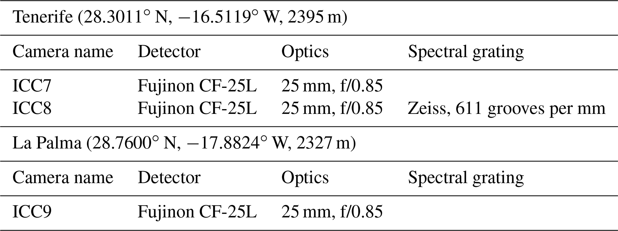
The Meteor Research Group (MRG) of the European Space Agency operates the double-station meteor camera system CILBO (Canary Island Long-Baseline Observatory) (Koschny et al., 2014). Several image-intensified video cameras are operated on Tenerife at the Izaña Observatory and on La Palma at the Observatorio del Roque de los Muchachos. A photograph of one of the cameras is shown in Fig. 1. Table 1 provides details on the individual cameras and locations.

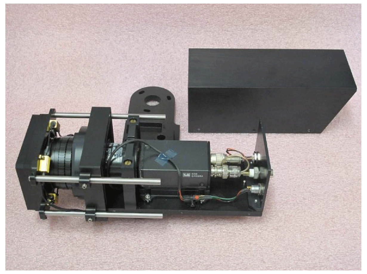
Figure 1 Photograph of one of the intensified video cameras equipped with a grating. The protective cover is removed and visible in the back. Power resistors to heat the grating can be seen on the left.

Table 1 Detailed information about CILBO stations and the camera setup.

The cameras ICC7 and ICC9 acquire videos with their lines of sight pointing to a point 100 km above the Earth's surface, at a location between the two islands, at 28.5533^∘ N and −17.1667^∘ W. The so-called spectral camera ICC8 is offset to ICC7 by 23.0^∘ to capture the first-order spectrum of meteors passing through the field of view of camera ICC7. A technical overview drawing is shown in Fig. 2.

Figure 2 Technical drawing of one of the intensified video cameras.

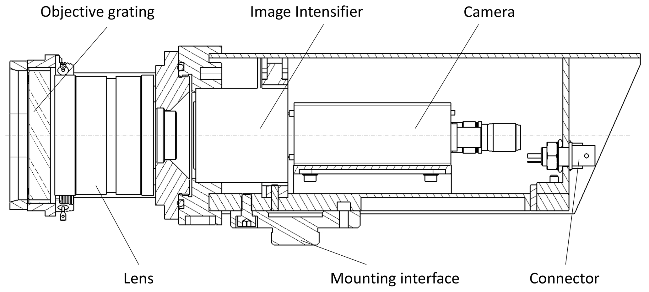
The camera systems use a low-distortion machine-vision lens from Fujinon, imaging the sky onto the entrance aperture of a second-generation image intensifier (DEP XX-1700). The intensifier has a spectral sensitivity from about 350 to 850 nm. It is fiber-coupled to a charge-coupled device (CCD), which is read out via a Toshiba Teli CS8310Bi PAL video camera. The PAL format has 576×768 pixels squared. Full frames are read out at a rate of 25 frames per second with 8-bit dynamical accuracy. With the given field of view the pixel scale is 2.3^′. A dew remover (type Kendrick) is wrapped around the objective lens to avoid dewing.

2.2 Control software

The core of the software is the detection software MetRec (Molau, 1999) that analyses the image streams from ICC7 and ICC9, independently from each other. The ICC8 camera image stream is read into a separate detection software called SpecRec on the computer of ICC7. In the case that the MetRec detection software of camera ICC7 detects a meteor, a hardwired trigger signal (RS232 serial port) is transferred to the ICC8 detection software. The image stream, including the three images acquired before the trigger signal arrived, is stored onto a hard disk. The MetRec software stores for each individual frame of each detected meteor event the right ascension and declination of the photometric center of the meteor and the magnitude. It also stores an estimate of the cloud coverage with 1 min accuracy. The computers are synchronized to a network-provided time signal every 2 min. A more detailed description of the CILBO setup and its cameras is available in Koschny et al. (2013b).

2.3 System performance

Since the start of operations in 2012, the cameras ICC7 and ICC8 have individually recorded over 90 000 meteor events, as indicated in Table 2. To apply the wavelength calibration to these events, the calibration routine we have developed requires that both zero-order images recorded by ICC7 and first-order spectra from ICC8 be available simultaneously (further explained in Sect. 4). About 14 000 were recorded by both systems simultaneously. The distribution of these events per year is listed in the column “Simultaneous events” in Table 2.

Table 2 Meteor events acquired from ICC7 and ICC8 systems since the year 2012. The columns “ICC7 events” and “ICC9 events” give the number of events recorded by ICC7 and ICC9, respectively. The column “Simultaneous events” gives the number of events recorded simultaneously by both ICC7 and ICC9. The last row gives the total number of events recorded since 2012.

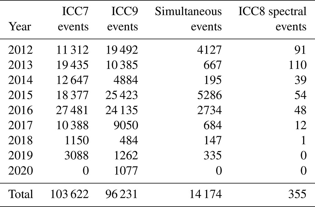
See Koschny et al. (2017) for a more detailed analysis covering 2012 to 2017. The 3D trajectory and heliocentric orbits of these meteoroids were computed using the MOTS (Meteor Orbit and Trajectory Software) code (Koschny and Diaz del Rio, 2002; Koschny et al., 2015b). The column “ICC8 spectral events” in Table 2 refers to the identified full spectra obtained. In this paper, we focus on the analysis from 2012 to 2017, as afterwards the transmissivity of the grating began to degrade. We have also excluded spectra that are not fully contained in all frames of the meteor event.

3 Radiometric correction and background subtraction

Each detected meteor event results in a number of bitmap (BMP) image files for ICC7 and ICC8, as well as an “information file” for ICC7 which contains measurement results for the meteor. The image files contain the three images acquired before the first detection of the event, as well as three images after the meteor event is lost.

As the CILBO setup did not foresee a camera door or shutter, a dark current image is only available from the time of the initial setup of the overall system in 2012. A flat-field image is produced synthetically by taking the median values for each pixel of an image sequence obtained on a clear night and then used throughout the years. First, all images, including the pre- and post-images, are radiometrically corrected by dark current subtraction and the flat-field division.

To compensate for acquisitions taken during cloudy conditions or during dawn or dusk, the six radiometrically processed pre-event and post-event images are stacked together into a background image: for each pixel, the median value of the six available pixels is taken.

Each radiometrically processed image in the meteor sequence is then subtracted by this background image. This operation also subtracts the stars from the images and would result in a low background image in the case that no spectrum is visible. A so-called total image is created by selecting for each pixel location the median pixel value of all images of the meteor sequence obtained so far. The total image provides a summary of the full meteor event and allows having a quick look at an event to judge the spectrum brightness.

The obtained image sequences, as well as the total image, dark current, and flat field, are stored in a single FITS-formatted file referenced as the level-0 dataset (see Sect. 9 for a detailed description).

4 Wavelength determination

Different to other algorithms described so far (Borovicka, 1994a; Dubs and Schlatter, 2015), our algorithm determines the pixel position as a function of wavelength in the ICC8 image, computed from the position in the zero-order image from ICC7. This is done by taking the angular offset between the two cameras into account. During the operational period of the cameras, this angular offset was derived several times from measurements and confirmed to be stable. The basic idea of this step can be best compared to the two-dimensional diffraction formula as we know it from the single-slit optical diffraction experiment.

$$\begin{array}{}\text{(1)}& \sin \mathit{\theta }=\mathit{\lambda }/d\end{array}$$

Knowing the wavelength λ and the slit width d, one can compute the angle θ and thus the location of the maxima and minima.

Assuming Fraunhofer's diffraction at the grating, the light of a star or meteor is considered parallel entering light rays, and its resulting diffraction can be expressed using the three-dimensional grating formula as provided in Eq. (2).

$$\begin{array}{}\text{(2)}& \overrightarrow{v^{\mathrm{Lens}}\left(\mathit{\lambda }\right)}=\left(\begin{array}{c}-x^{\mathrm{grating}}-\left(n\mathit{\lambda }d\right)\\ -y^{\mathrm{grating}}\\ \sqrt{\mathrm{1}-{\left(x^{\mathrm{grating}}+\left(n\mathit{\lambda }d\right)\right)}^{\mathrm{2}}-{\left(y^{\mathrm{grating}}\right)}^{\mathrm{2}}}\end{array}\right),\end{array}$$

where

• $\overrightarrow{v^{\mathrm{lens}}\left(\mathit{\lambda }\right)}$ represents the direction of the diffracted light with respect to the lens for each wavelength λ;

• (x,y)^grating represents the coordinates on and in the plane of the grating, at which the light enters;

• n is the grating order, which has +1 as a nominal value;

• λ is the wavelength (in meters);

• d is the groove density (in number of grooves per meter).

With the information from ICC7, especially the right ascension and declination of the meteor, the zero order, for each individual frame, this diffraction vector $\overrightarrow{v^{\mathrm{Lens}}\left(\mathit{\lambda }\right)}$ for any wavelength λ can be calculated. To derive the (x,y) coordinates at the CCD frame, a sequence of reference frame transformations has to be applied. We further assume that all reference frames are right-handed ones and that the reference frames' z axes are aligned with each other, in particular the CCD, the optical, and the grating z axes.

As a first step, we have to derive the (x,y)^grating coordinates of Eq. (2) by applying the following reference frame transformations.

• ℱ_celestial⟶ℱ_{local horizon}
  This transformation converts a meteor position (right ascension and declination in J2000, as obtained from ICC7 information) for a given time from the Earth-centered celestial frame into an observer-centered frame (altitude, hour angle), with the horizon as the fundamental frame, using the Python routine eq2hor.

• ℱ_{local horizon}⟶ℱ_grating
  This transformation converts a meteor position (altitude and hour angle) for a given time from the observer-based frame into a grating-centered reference frame. This conversion requires knowledge of the azimuth and elevation of the +x axis and +y axis of the grating, respectively. Assuming that it is identical to the optical axis of the complete camera system, it can be computed from the right ascension and declination of the center of the field of view at any given time. The boresight angle, the angle that the z axis of the grating is tilted, allows for a non-horizontal plate. Unfortunately, this value was not measured at the time of the CILBO installation and we use a rotation value of −11.0^∘ as a best-fit value in the z axis. The tilt angle describes a rotation of the grating, a rotation of the x–y plane of ℱ_grating perpendicular to the +z axis of the grating. If these angles are known, a transformation matrix can be constructed to convert any vector in the horizontal frame into a vector in the grating frame as follows.

  $$\begin{array}{}\text{(3)}& \begin{array}{rl}{\mathit{x}}^{\mathrm{grating}}& =M_{\mathrm{azimuth}}\cdot M_{\mathrm{elevation}}\cdot M_{\mathrm{boresight}}\cdot M_{\mathrm{tilt}}\\ & \cdot {\mathit{x}}^{\mathrm{local}\mathrm{horizon}}\end{array}\end{array}$$

• ${\mathcal{F}}_{\mathrm{grating}}⟶{\mathcal{F}}_{\mathrm{lens}}^{\mathit{\lambda }}$ can be determined with Eq. (2) and produces a vector for each wavelength λ.

  From the vector $\overrightarrow{v^{\mathrm{lens}}\left(\mathit{\lambda }\right)}$ one could directly transform into the CCD frame and obtain the (x, y) coordinates of the image by normalizing the z component of $\overrightarrow{v^{\mathrm{lens}}\left(\mathit{\lambda }\right)}$ to 1. From the known field of view of the camera, one can construct vectors from the CCD center to the field-of-view corners assuming again that the z component equals 1. From these relations we can derive the x position and y position in the CCD frame of the meteor directly.

We follow a different approach and transform the obtained vectors back in an inverse transformation into ${\mathcal{F}}_{\mathrm{celestial}}^{\mathit{\lambda }}$ by applying the inverse matrices of Eqs. (2) and (3). As a result, we obtain the celestial coordinates for each wavelength. With knowledge of the plate constant of the camera, these coordinates can be directly transformed into the image (x, y) coordinates. We used the Python method all_world2pix() of the astropy.wcs class. To allow this last transformation, we use the web service offered by astrometry.net (Lang et al., 2010) (http://nova.astrometry.net, last access: 31 March 2023) to obtain a registered image. This registration was done once with an image under good viewing conditions. As the web-service registration also takes the geometric distortions into account, the algorithm does not need to apply any additional distortion correction routines.

The calibration step results for each frame in a list of wavelengths and its corresponding digital value at the computed image position and is stored in a single FITS file labeled as the level-1 dataset (see Sect. 9 for a detailed description).

It is noted that the accuracy of our algorithm – determined through the correct identification of the (x, y) position of a maxima for a chemical element – was not always satisfactory. As the bright pixels representing the zero-order meteor in ICC7 are spread over many pixels, a centroid algorithm is used in METREC that did not always correspond to the center pixel of the meteor as visually observed. The difference was within a few pixels, but the impact on the overall accuracy of the algorithm was too large to neglect. The problem was corrected in a later processing step (see Sect. 7.2) by adding the wavelength itself as one of the Bayesian parameters.

5 Spectral calibration

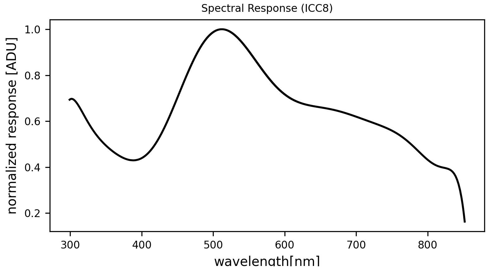
5.1 Spectral response of ICC8

The spectral response curve for ICC8 was derived from images containing the first-order spectrum of Vega.

Vega is an A0-type star with a well-known emission spectrum in the visible range. A reference spectrum of Vega was taken from the STIS CALSPEC Archive at https://archive.stsci.edu/hlsps/reference-atlases/cdbs/current_calspec (last access: 31 March 2021). To obtain an ICC8 Vega spectrum, four frames acquired on 4 consecutive days were selected. Each frame is then radiometrically processed and the wavelengths are derived as provided in Sects. 3 and 4. The final observed Vega spectrum is the median of the four calibrated and atmospheric-corrected spectra. The ICC8 spectral response curve is the ratio between the final observed spectrum and the reference spectrum, fitted with a 12th-order polynomial and normalized to 1, as shown in Fig. 3. To validate the ICC8 spectral response, acquired spectra of Algol, Castor, Deneb, Elnath, and Vega underwent our calibration pipeline and were compared to the spectra provided in CALSPEC or HyperLeda (http://leda.univ-lyon1.fr/, last access: 31 March 2021).

Figure 3 Normalized ICC8 spectral response curve.

5.2 Correction of atmospheric attenuation

As the light emitted from the ablation process undergoes atmospheric extinction, we apply a correction to the spectral response curves as obtained in Sect. 5. The scattering and absorption correction is applied to each individual frame and depends on the exact observation geometry, especially the zenith angle of the observed meteor θ_met and the optical thickness b_met of the atmosphere. The extinction law can be described as a correction vector (Appenzeller, 2013), as follows:

$$\begin{array}{}\text{(4)}& \overrightarrow{v_{\mathrm{corr}}}={\displaystyle \frac{\overrightarrow{F_{\mathrm{0},\mathrm{met}}}}{\overrightarrow{F_{\mathrm{met}}}}}={\displaystyle \frac{\mathrm{1}}{\exp \left(\frac{\overrightarrow{-b_{\mathrm{met}}}}{\cos \left({\mathit{\theta }}_{\mathrm{met}}\right)}\right)}},\end{array}$$

where $\overrightarrow{F_{\mathrm{met}}}$ represents the intensity of each feature of the observed meteor spectrum and $\overrightarrow{F_{\mathrm{0},\mathrm{met}}}$ the intensities of the true, atmospheric-corrected, spectrum. The atmospheric optical thickness is a coefficient specifying the attenuation of light through the atmosphere; $\overrightarrow{b_{\mathrm{met}}}$ is a vector varying with wavelength. In the case that we consider only scattering contributing to the atmospheric extinction and the aerosol absorption, $\overrightarrow{b_{\mathrm{met}}}$ =$\overrightarrow{b_{\mathrm{sca}}}$ is obtained as in Eq. (5), with N_gas the column number density of gas molecules (obtained using Eq. 6), σ_sca the scattering cross section of gas molecules (obtained with Eq. 7), and AOT the contribution of the aerosol optical thickness. The AOT is taken from NASA's AERONET (NASA's AERONET database is found at https://aeronet.gsfc.nasa.gov/new_web/aerosols.html, last access: 1 March 2023). The file which contained the data used was named “aerosol optical depth” (AOD) with precipitable water and Ångström parameter. database. The data were recorded by an AERONET sun photometer in Izana, Tenerife, located at around 1.17 km ground distance from our ICC8 camera. The data are provided at discrete, irregular intervals from 340 to 870 nm.

$$\begin{array}{}\text{(5)}& {\displaystyle }\overrightarrow{b_{\mathrm{met}}}=\overrightarrow{b_{\mathrm{sca}}}=N_{\mathrm{gas}}\cdot {\mathit{\sigma }}_{\mathrm{sca}}+\mathrm{AOT}\text{(6)}& {\displaystyle }{N}_{\mathrm{gas}}={\displaystyle \frac{p_{\mathrm{bottom}}-p_{\mathrm{top}}}{m_{\mathrm{gas}}\cdot g}}\text{(7)}& {\displaystyle }{\mathit{\sigma }}_{\mathrm{sca}}\left(\mathit{\lambda }\right)={\displaystyle \frac{\mathrm{24}{\mathit{\pi }}^{\mathrm{3}}}{N_L^{\mathrm{2}}}}{\displaystyle \frac{(n^{\mathrm{2}}-\mathrm{1}{)}^{\mathrm{2}}}{(n^{\mathrm{2}}+\mathrm{2}{)}^{\mathrm{2}}}}{\displaystyle \frac{(\mathrm{6}+\mathrm{3}\mathit{\delta })}{(\mathrm{6}-\mathrm{7}\mathit{\delta })}}{\displaystyle \frac{\mathrm{1}}{{\mathit{\lambda }}^{\mathrm{4}}}}\approx {\displaystyle \frac{C}{{\mathit{\lambda }}^{\mathrm{4}}}}\end{array}$$

Here, m_gas is the air mass (obtained for dry-air conditions, 28.96 g mol⁻¹) and g the gravitational acceleration (9.806 m s⁻²), both considered constant through the atmosphere. p_bottom and p_top are the pressures at the altitudes of the atmosphere corresponding to the beginning and end of the meteor ablation. In Eq. (7), n is the gas refractive index (assumed constant), N_L is Loschmidt's number (2.54743 10²⁵ m⁻³), and δ is the gas depolarization constant (0.03 for terrestrial air, ignoring the λ dependence).

As several of the parameters depend on the line of sight between the station ICC8 and the meteor location (and thus the meteor altitude), the atmospheric correction is applied to each individual frame of a meteor event. The altitude-varying parameters are computed as follows: g and n are approximated as constants between ICC8 (the troposphere) and the meteor location (the thermosphere).

Figure 4 Example of ICC8 spectral profile before (black), after the instrument sensitivity (spectral response) correction (blue), and after the atmospheric extinction correction (yellow).

p_top is calculated using Eq. (8):

$$\begin{array}{}\text{(8)}& p=p_{\mathrm{0}}\cdot {\left(\mathrm{1}-{\displaystyle \frac{L\cdot h}{T_{\mathrm{0}}}}\right)}^{\left(\frac{g\cdot M}{L\cdot R_{\mathrm{0}}}\right)},\end{array}$$

where p₀ is the SI standard pressure (101325 Pa), L the temperature lapse rate (9.76 K km⁻¹, dry air), T₀ the SI standard temperature (288.16 K), M the molar mass (0.029 kg mol⁻¹, dry air), and R₀ the universal gas constant (8.314 J mol K⁻¹).

A detailed discussion of the assumptions, especially related to the atmospheric values, the improvements obtained, and potential further improvements of the correction using the atmospheric extinction correction, can be found in Vicinanza et al. (2021). Figure 4 shows a spectral profile before and after the atmospheric extinction correction was applied.

This calibration step results for each frame of a meteor event in a list of wavelengths and the corresponding spectral-calibrated and atmospheric-corrected value are stored in a single FITS file labeled as the level-3 dataset (see Sect. 9 for a detailed description).

6 Intensity calibration

The aim of the intensity calibration is to convert the spectral intensity, measured in CCD pixel counts often expressed as arbitrary digital units (ADU), to SI physical units (W m⁻² nm⁻¹). This allows inferring the true and absolute composition of elements in a meteoroid during the extraction of the line intensities of individual chemical elements (as will be described in Sect. 7). The intensity calibration is done in two steps following Jenniskens (2007): the calculation of the zero-point bias and the estimation of the coefficient of intensity calibration.

The calculation of the zero-point bias involves a photometric calibration. This is performed using the observations of A0V standard stars, simultaneously recorded in the background of meteor observations. We used Vega, which has a V-band magnitude m of approximately 0. Knowing the spectral intensity of Vega observed from ICC8, expressed as the sum of ICC8 pixel brightness ∑F, the zero-point bias C is obtained using the relation

$$\begin{array}{}\text{(9)}& m=C-\mathrm{2.5}\log \left(\sum F,\text{in ADU}\right),\end{array}$$

where ∑F is Vega's sum of the pixel brightness, and C is the zero-point bias we want to obtain. By applying this step to our set of CILBO observations, a value of 10.81±0.1 was obtained for the zero-point bias. Theoretically, this step should be performed separately for each individual meteor event using the stars observed in the meteor's background. However, since it was observed that the zero-point bias remains approximately constant throughout different events, a constant term was applied during our research to the calibration of all events.

The zero-point bias is then used for the estimation of the coefficient of intensity calibration, k, according to the relation below (Jenniskens, 2007):

$$\begin{array}{}\text{(10)}& k={\displaystyle \frac{\mathrm{3.67}\times {\mathrm{10}}^{-\mathrm{11}}\times {\mathrm{10}}^{-C/\mathrm{2.5}}}{\mathrm{EW}}},\end{array}$$

where C is the zero-point bias and EW is the equivalent width of the spectral response (measured as the full-width half-maximum) of the camera (see Fig. 3) and allows performing a correction for the instrument aperture. Equation (10) is obtained knowing that the zero-magnitude A0V standard star Vega has a flux of $\mathrm{3.67}\times {\mathrm{10}}^{-\mathrm{11}}$ W m ⁻² nm⁻¹ at 548.3 nm (V band). On average, the coefficient k, separately calculated for each event, was around $\mathrm{2}\times {\mathrm{10}}^{-\mathrm{17}}$ W m⁻² nm⁻¹ ADU⁻¹. Once this coefficient is obtained, the calibrated meteor spectral intensity (at each wavelength λ) is obtained from the observed meteor flux F following the relation

$$\begin{array}{}\text{(11)}& F_{\mathit{\lambda }}^{\mathrm{cal}}=k\cdot f\cdot \left(\sum F,\text{in ADU}\right)=k_{\mathrm{corr}}\cdot \left(\sum F,\text{in ADU}\right).\end{array}$$

F is the average of the flux over 10 binned pixel rows. Since the coefficient k is obtained using Vega star observations and we want to perform the intensity calibration on meteor observations, the correction factor f is needed. This accounts for the dependence of the intensity calibration coefficient k_corr on the exposure time of the star measurement compared to the exposure time of the meteor measurement.

$$\begin{array}{}\text{(12)}& f={\displaystyle \frac{\text{exposure time star}}{\text{exposure time meteor}}}\end{array}$$

The exposure time of a Vega observation is equal to the observation time for the entire meteor event. Since we perform the intensity calibration for each meteor frame (10 binned pixel rows), the exposure time of the meteor is a ratio of the time delay between consecutive frames. Our cameras have a frame rate of 25 FPS and thus a 0.04 s interval between consecutive frames (Koschny et al., 2013b). The exposure time of the meteor in each frame can thus be obtained as

$$\begin{array}{}\text{(13)}& \begin{array}{rl}\text{exposure time meteor}& ={\displaystyle \frac{\mathrm{0.04}\mathrm{s}}{\mathrm{\Delta }{y}_{i,i+\mathrm{1}}}}\\ & \cdot \text{number binned pixel rows},\end{array}\end{array}$$

where $\mathrm{\Delta }{y}_{i,i+\mathrm{1}}$ is the difference in y coordinate between consecutive MetRec recordings and depends on the meteor speed.

In conclusion, the coefficient of intensity calibration k – used to convert the spectral intensity of meteor spectra from some arbitrary digital units (ADU) to SI physical units (W m⁻² nm⁻¹) – was considered constant for diverse observations of the same meteor event, while it changed between different meteor events. The change mostly depends on the different exposure times of different meteor events (related to the different meteor speed), the different conditions of atmospheric extinction encountered at different meteor entries, and the optical and camera characteristics (as obtained through the zero-point bias). In our cases, the coefficient k was of the order of $\mathrm{2}\times {\mathrm{10}}^{-\mathrm{17}}$ W m⁻² nm⁻¹ ADU⁻¹.

7 Extraction of line intensities of individual chemical elements

To determine the chemical elements and their contribution to a meteor spectral profile, a line-by-line emission simulation has to be executed for each potential chemical atom, molecule, or oxide. The atomic behavior of each species needs to be modeled, taking into account a number of model input parameters, especially the ablation temperature and the chemical element number densities. As the selection of slightly different input parameters results in different spectral profiles that might or might not match a meteor spectral profile from the level-3 datasets (see Sect. 9.3), we have to solve an optimization problem. The CILBO calibration pipeline uses the Plasma Radiation Database (PARADE) line-by-line emission simulation tool (Smith, 2006). We use the Bayesian formalism to solve the optimization problem, and the PARADE tool is called from within the Bayesian method; both are discussed in the following sections.

7.1 The Plasma Radiation Database

The synthetic spectra are produced by ESA's Plasma Radiation Database (PARADE) tool, originally used to simulate variation of probe entries into planetary atmospheres (Smith, 2006; Pfeiffer et al., 2003). PARADE calculates the energy state transitions in atoms and molecules and provides the emission coefficient ϵ in radiance W m⁻³ sr⁻¹ m⁻¹.

While the number of gaseous elements was originally restricted to the main atmospheric constituents of the atmospheres of Titan, Earth, and Mars, several new species have been added to support our spectral analysis activities for the CILBO acquired spectra. A detailed discussion is given in Loehle et al. (2021), extending the available species to include Na, K, Ti, V, Cr, Mn, Fe, Ca, Ni, Co, and Li. The positional information of an emission (or absorption) line is defined by the energy gap between the electron excitation levels as defined by, e.g., Herzberg (1950).

$$\begin{array}{}\text{(14)}& \mathrm{\Delta }E=h\mathit{\nu }={\displaystyle \frac{hc}{\mathit{\lambda }}}\end{array}$$

The energy levels of atoms are exclusively defined by their electron configuration and energy levels. These can be determined from the NIST database (Ralchenko and Kramida, 2020) directly. For molecules, the vibration and rotation of the nuclei are additional parameters to consider. A simple radiation model for diatomic molecules based on a Boltzmann distribution of the vibrational bands and under the assumption of thermal equilibrium is presented in Eq. (15) (Loehle et al., 2021).

$$\begin{array}{}\text{(15)}& {\displaystyle \frac{N_J}{N}}={\displaystyle \frac{hc{A}_{v,u}}{kT}}\left(\mathrm{2}(J-\mathrm{1})+\mathrm{1}\right)e^{\left(-A_{v,u}(J-\mathrm{1})(J+\mathrm{1})\mathrm{100}\frac{hc}{kT}\right)}\end{array}$$

Here, h denotes the Planck constant, k the Boltzmann constant, c the vacuum speed of light, A_v,u the Einstein coefficient for a spontaneous emission from a lower to a higher state N_J, J the rotational quantum number, and T the temperature. In addition, we have further extended the PARADE tool to the following molecules: CO, CO₂, AlO, CaO, FeO, MgO, NO, and TiO.

To avoid the repetitive execution of PARADE simulations in the upcoming processing step (see Sect. 7.2), a database is created containing for each species the emission profile over the spectral regime for temperatures in a temperature range from 2000 to 15 000 K in a 50 K granularity. When building up the synthetic emission lines, FeI is processed over the full spectrum, as well as over a limited spectral width that explicitly covers the FeI (15) multiplet response, ranging between 520 and 550 nm. The modeled spectra include the contribution of the Planck background at the individual temperatures; for details see Loehle et al. (2021). In summary, the following atoms, molecules, and ions are available in our database: NaI, MgI, FeI, FeI(15), CaI, SiI, AlI, MnI, CrI, Ar, C₂, CH, CN, CO₂, FeO, CaO, AlO, MgO, O₂, OH, TiO, Na⁺, Mg⁺, Fe⁺, Ca⁺, and Ar⁺.

7.2 Optimization of the spectral fitting using the Bayesian methodology

The PARADE tool allows computing the radiative emission of gas species by calculating the line position as well as its intensity and distribution, i.e., the line profile (Herzberg, 1950; Loehle et al., 2021; Rudawska et al., 2020), for a given temperature and given number density of a selected gas species.

Taking the reduced line profiles as obtained after the calibration steps (the dataset level 3), a fit to the set of simulated results from the PARADE tool must be found. To solve this inverse problem we use the Bayesian treatment of the inference, Bayes' theorem, and apply it to the meteor ablation process.

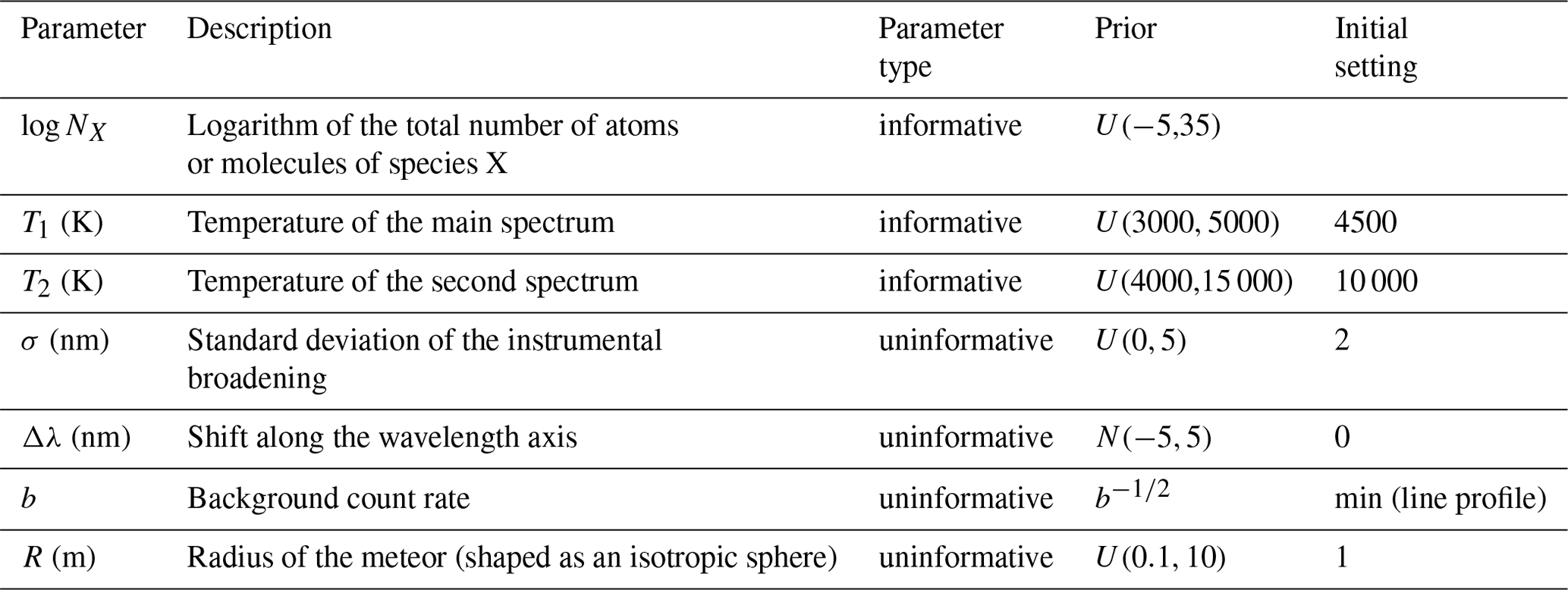
Having priors is of key importance in the Bayesian framework as priors express our existing knowledge about the parameter space. Parameters for which a lot of knowledge is available are named informative priors in the Bayesian framework. They are updated by the algorithm based on new data provided. In our case, we have three informative priors, all being input parameters to the PARADE simulation. The first is the total number of atoms or molecules of a gaseous species directly relating to the maximum values of the simulated line profiles. We consider this number to be uniformly distributed. The temperature of a meteor ablation process is an informative prior and we assume a uniform distribution. Following the identification of two distinct thermal components in the meteor ablation by Jenniskens (2007), we take two distinct temperature components, T₁ and T₂, as informative priors.

Uninformative or ignorance priors are very diffuse and do not constrain the parameters. These are used when we do not have a lot of knowledge about the parameter beforehand and are not used within the PARADE simulations. We use three uninformative priors in our framework.

• The PARADE tool takes into account several line-broadening effects within its simulation like the Van der Waals, or natural or Stark broadening. As the errors associated with these models are not yet fully quantified, we have introduced the standard deviation of the instrumental broadening, σ, as an uninformative prior and consider its distribution function uniform.

• We have reported in Sect. 5 an uncertainty in the position measurement of the meteor center that we are not able to characterize further and have therefore introduced as an uninformative prior the uncertainty along the wavelength axis, Δλ, of the measured line profiles. For this uninformative prior we also assume a Gaussian distribution.

• Moreover, the line profile itself constitutes a level of signal noise that propagates through the algorithms (as described earlier) and is difficult to characterize. We thus introduce another uninformative prior, the line profile background b, assuming a Gaussian distribution.

Finally, we need to convert the modeled synthetic spectra in irradiance (W m⁻³ sr⁻¹ nm⁻¹) into radiance (W m⁻² nm⁻¹). This is done by performing a solid angle conversion assuming the meteor to have the shape of an isotropic sphere (Jenniskens, 2007). We introduce a final uninformative prior, the size of the ablating body, the meteor, in the direction of flight R, assuming a uniform distribution. From R we derive the luminous area of the radiating body as π*R².

Table 3 lists all priors and their initial settings.

Table 3 Overview of the parameters of our model, the choice of prior, and initial settings.

The Bayesian treatment of the inference, Bayes' theorem, can be written as

$$\begin{array}{}\text{(16)}& P\left(\mathit{\theta }\right|Y)={\displaystyle \frac{\mathcal{L}\left(Y\right|\mathit{\theta }\left)\mathit{\pi }\right(\mathit{\theta })}{\mathit{\pi }\left(Y\right)}}.\end{array}$$

P(θ|Y) denotes the probability of a model applied over a parameter space θ, in our case the temperature, the instrumental line broadening, the uncertainty in the wavelength, and the background count rate, given a set of data samples $Y=(y_{\mathrm{0}},y_{\mathrm{1}},\mathrm{\dots }{y}_N)$. y_i denotes line intensities simulated for the individual species. In the literature, P(θ|Y) is typically referred to as the posterior.

π(θ) represents the probabilities of the parameters, the prior. Finally, π(Y), typically referred to as the evidence, represents the probabilities of the simulated line profiles.

ℒ(Y|θ), the likelihood, is the product of the probability of the individual data points,

$$\begin{array}{}\text{(17)}& \mathcal{L}\left(Y\right|\mathit{\theta })=\prod _i^{N}P(y_i\left|\mathit{\theta }\right),\end{array}$$

given an independent set of data points $Y=(y_{\mathrm{0}},y_{\mathrm{1}},\mathrm{\dots }{y}_N)$ sampled over $X=(x_{\mathrm{0}},x_{\mathrm{1}},\mathrm{\dots }{x}_N)$.

Assume we have a parameterized model f(x|θ) which models the data Y for given parameters θ and explanatory variable X, in our case the wavelength. With this model we can then calculate the probability of generating an observed data point P(y|θ), also known as the likelihood ℒ(y|θ). If we have an independent set of data points $Y=(y_{\mathrm{0}},y_{\mathrm{1}},\mathrm{\dots }{y}_N)$ sampled over all wavelength $X=(x_{\mathrm{0}},x_{\mathrm{1}},\mathrm{\dots }{x}_N)$, the total likelihood is the product of the probability of the individual data points.

As the measured line profiles from the gaseous species are derived from CCD images, and thus photon counts, the likelihood of the probability distribution line profiles over wavelength is given by a Poisson distribution.

$$\begin{array}{}\text{(18)}& \mathcal{L}\left(Y\right|\mathit{\theta })=\prod _i^N{\displaystyle \frac{f\left(x_i\right|\mathit{\theta }{)}^{y_i}\exp \left(f\left(x_i\right|\mathit{\theta })\right)}{y_i\mathrm{!}}}\end{array}$$

Instead of using the likelihood as in Eq. (18), it is common to work with the log-likelihood, as that reduces the product to a sum over the data points. In the Poisson case, the negative log-likelihood is given by

$$\begin{array}{}\text{(19)}& -\ln \mathcal{L}\left(Y\right|\mathit{\theta })=\sum _i-y_i\ln (f\left(x_i\right|\mathit{\theta })+f(x_i\left|\mathit{\theta }\right)+\ln \left(y_i\mathrm{!}\right).\end{array}$$

Before we can start the Bayesian framework, an initial guess of the synthetic spectrum is computed based on the values in Table 3. As we study the optically thin case (optical depth τ≪1) and use discreet temperature values, the final synthetic spectrum is then a linear combination of the individual emission spectra of each species as described in Eq. (20):

$$\begin{array}{}\text{(20)}& F_{\mathit{\nu }}^{\text{source}}\left(T\right)=\sum _i{N}_i{j}_{\mathit{\nu },i}\left(T\right),\end{array}$$

where $F_{\mathit{\nu }}^{\text{source}}$ is the flux vector of the complete source spectrum, i.e., the sum of the spectra of all species “i” at the source, N_i the number density of each species, and j_ν,i the temperature-dependent emission coefficient of element i. The elements' emission coefficients are retrieved from PARADE (introduced in Sect. 7.1). The flux vector F_ν comes from the meteor observations. The only unknowns of the equation are the number densities N_i.

The estimation of the number densities of the meteor's radiating elements is articulated in three sequential steps: a linear regression retrieval, a nonlinear least-squares initial solution, and the final Markov chain Monte Carlo (MCMC) parameter estimation.

For each species and each discreet temperature in our emission database (described in Sect. 7.1), the obtained spectral profile is further modeled into a set of synthetic spectra. These are obtained through different combinations of the parameters in Table 3, left free to vary within defined boundaries (“Prior” in Table 3). A linear solution of the parameters in Table 3 is then retrieved, estimating the Moore–Penrose pseudo-inverse of the matrix having on its rows the species' synthetic spectra obtained at each combination. By applying a linear regression, considering the ICC8 observed meteor spectrum as the dependent variable, a first estimate of the number density of all the species considered is obtained.

Using these linear estimates as a first guess, a nonlinear least-squares approach is used to obtain an even more accurate estimation of the number densities' initial solution. This provides the estimate of all the unknown parameters in Table 3, whose combination generates a complete synthetic meteor which best fits the ICC8 observed meteor spectrum. The nonlinear least-squares solution for the number densities, and other parameters, is determined using the Levenberg–Marquardt algorithm. Our approach is very similar to Benneke and Seager (2012), where Bayesian inference is used to retrieve and constrain the composition of exoplanet atmospheres from their transit spectra. These best-fit least-squares estimates are, however, only an initial solution and thus do not coincide with the final best-fit solution obtained at the end of the routine, after the Markov chain Monte Carlo (MCMC).

The least-squares parameter estimates are used as initial guesses for the successive MCMC. Using the MCMC sampling we estimate the posterior distribution of the parameters of the spectral model. The MCMC sampler approximates the posterior distribution by generating samples with a probability that is proportional to the posterior:

$$\begin{array}{}\text{(21)}& n\left(\mathit{\theta }\right)\mathrm{d}\mathit{\theta }\propto P\left(\mathit{\theta }\right|Y)\mathrm{d}\mathit{\theta },\end{array}$$

where n(θ)dθ is the number of samples between θ and θ+dθ. In MCMC methods we generate so-called Markov chains, which follow this distribution. A Markov chain is a random process which obeys the Markov property that a successive data point is only based on the most recent data point.

$$\begin{array}{}\text{(22)}& P\left({\mathit{\theta }}_i\right|{\mathit{\theta }}_{i-\mathrm{1}}\mathrm{\dots }{\mathit{\theta }}_{i-N})=P({\mathit{\theta }}_i\left|{\mathit{\theta }}_{i-\mathrm{1}}\right)\end{array}$$

We thus obtain not only a point estimate of the chemical composition of the meteor but also an estimate of the full probability distribution, giving a constraint on the range of abundances which could describe the meteor. During the MCMC, for each meteor event 1000 iterations are run. Each iteration models a different synthetic spectrum using parameters which are sampled around the nonlinear least-squares solution via MCMC affine-invariance sampling. We use the emcee Python package (Foreman-Mackey et al., 2013, 2019) that implements the affine-invariant ensemble sampler by Goodman and Weare (2010). The algorithm performed well under all linear transformations and is insensitive to covariances among parameters. The complete synthetic spectrum which best fits the ICC8 observed spectrum is inferred using Bayesian inference: the best-fit parameters represent those for which the posterior has the highest value. Specifically, the inference returns the combination of parameters for which the modeled (synthetic) spectra best fit the observed spectra (data).

8 Spectral calibration discussed for one meteor event

This section describes the individual processing steps and intermediate results based on the meteor event 20131214T041302. The meteor presented was classified by METREC to belong to the Geminid shower and was observed in December 2013. The meteor itself and its spectral signature were detected in 24 individual frames in cameras ICC7 and ICC8, respectively. The maximum apparent magnitude was −1.7. The level-1 FITS file contains the individual frames and total image (shown in Fig. 5).

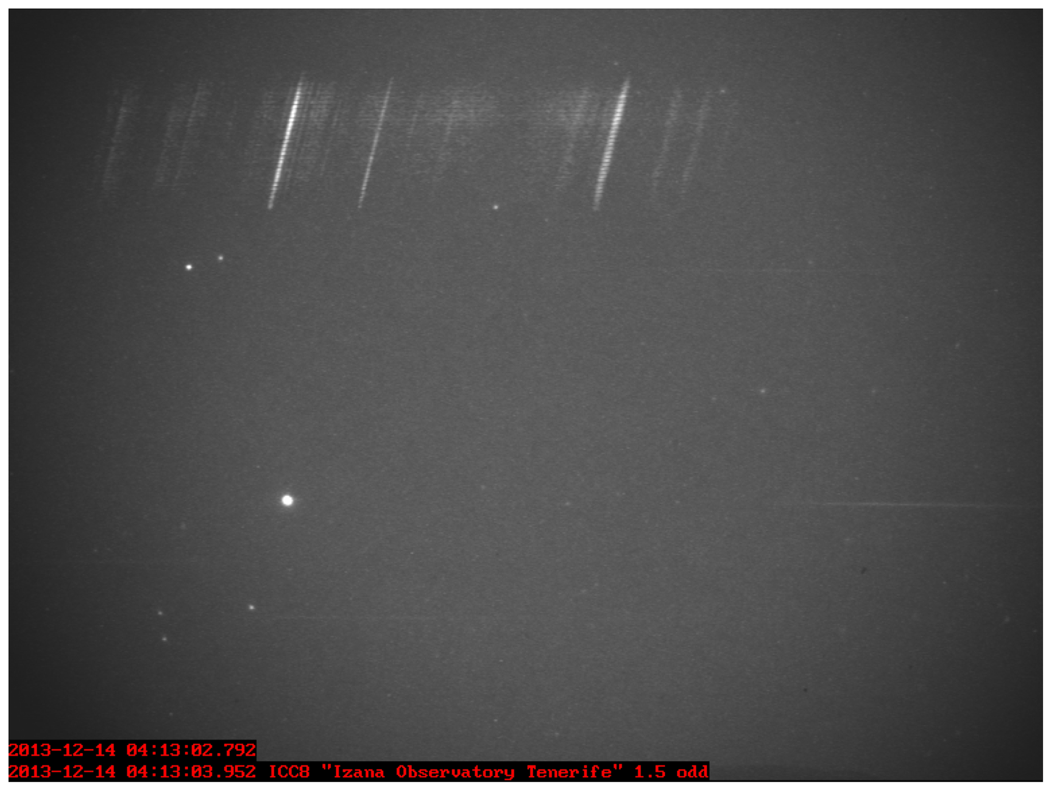
Figure 5 Total image (max pixel value over all frames) of event 20131214T041302 as observed by camera ICC8.

In the next processing step, the (x, y) position for each wavelength is determined frame by frame, resulting in an line plot representing the meteor spectrum intensity. The profile is further spectrally calibrated and corrected for atmospheric effects, resulting in a level-2A FITS file. The level-2B FITS file contains the final calibration product, after the intensity calibration is applied, in radiance (W m⁻² nm⁻¹). The unprocessed and calibrated profile of the brightest frame, frame 20, is shown in Fig. 6.

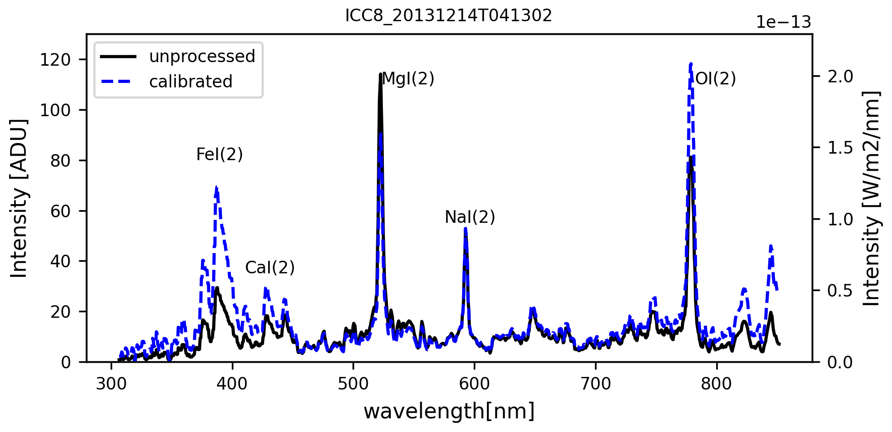
Figure 6 Unprocessed (black line) and calibrated (blue dashed) profile plot of frame 20 (20131214T041302).

The 1000 MCMC iterations of the ablation processes as part of the Bayesian interference algorithms are based on the priors and initial settings as given in Table 3 (see Sect. 7.2). In our setup – thus also applicable for this example – the initial settings used for the chemical elements are computed by a least-square fitting algorithm, and the resulting values are given in Table 4. The selection of chemical elements, the main temperature, and the secondary temperature (see Sect. 7.2) proved stable through the processing of all meteor events. In the future, we might apply a different larger selection of elements, i.e., when processing meteor events of a dedicated meteor shower.

Table 4 Initial settings for elements and final results obtained. The number density is given (cm⁻³).

After the Bayesian interference algorithm and MCMC run have finished simulations and the best fit is available, a check on the convergence of all parameters used in the simulation is needed. This is done by the visual analysis of the so-called corner plot that is produced by the data pipeline for each meteor event. The corner plot – see Fig. 7 in Foreman-Mackey (2016) – visualizes the posterior probability distribution of the parameters in diagonals and the covariances between the parameters of the Monte Carlo iterations on the non-diagonals. The distribution of most parameters indicates a Gaussian distribution around a best estimate. A clear peak is visible for MgI, but two side maxima are visible. This might indicate either a higher level of noise or interference with another chemical element. From Fig. 10, we could argue that CrI could interfere with MgI.

Figure 7 Example of a corner plot, showing the posterior distribution on the diagonals and covariances of a few selected parameters in the non-diagonals.

This validation step is currently the only manual step needed in the calibration pipeline. In the case that a parameter is not converging, the parameter needs to be taken out of the simulation and a re-run of the simulation is needed.

• The two temperature regimes result in temperatures of 4000 and 9000 K. The variations in the chain plots are marginal and we consider the two temperatures to be an important result of our analysis.

• The chemical elements Fe, Na, Mg, Si, Cr, Ti, K, CaO, FeO, N₂, Ca⁺, Fe⁺, MG⁺, O, and N converge well.

• The parameters background, wavelength shift, and radius_sphere are also contained in the corner plots (not shown in Fig. 7). The background is a proxy for the noise level in the spectral profiles, and the wavelength shift is an indicator for an additional correction of the wavelength to achieve a good result (in the presented case fewer than two pixels); radius_sphere is the radius of the meteor's luminous area. According to Jenniskens (2007), the meteor is considered an isotropic sphere; i.e., the radiating area perpendicular to the observer has the same value across all directions of the observer, and thus the luminous area equals π⋅radius_sphere².

At the end of our event analysis, the data allow the comparison of the observed spectrum to the simulated spectra obtained for the total images and the brightest frame. Figure 8 shows the obtained plots demonstrating the fitting algorithm. Most maxima in the observed spectrum are well fitted. Also, the broad bands are fitted well, but some overshooting is observed between 550 and 650 nm. The intensity of the individual frame is given on the right y axis and is less intense than in the total image. The reader shall note that the red line in Fig. 8 represents the calibrated spectra (W m⁻² nm⁻¹) of the brightest frame and is thus much smaller than the corresponding black line that represents the energy of the overall meteor event (thus of all the frames).

Figure 8 Calibrated spectrum (black line) and fitted spectrum (blue) of the total image of event 20131214T041302.

Table 4 contains the resulting number densities in the right column that can be interpreted in the following way.

• From the meteoric elements, the highest number density is obtained for Si.

• The Na content is relatively small, especially in comparison to the Fe and Mg. As the sodium is a direct indicator of the fluffiness of the meteoroid and thus its parent body (Abe et al., 2020), this is an indication that the meteoroid might be composed of stronger material without small grains. Our observation confirms earlier studies from, e.g., Abe et al. (2020) and Vojáček et al. (2019).

• Borovička (2010) and Abe et al. (2020) provided ratios of $\mathrm{Na}/\mathrm{Mg}$ of 0.023 and 0.067, respectively. The value we obtain for the event discussed is 0.0003 and deviates thus a lot.

• Borovička (2010) and Abe et al. (2020) provided ratios of $\mathrm{Fe}/\mathrm{Mg}$ of 0.32 and 0.3, respectively. The value we obtain is 0.09, a factor of 3 smaller. Borovička (2010) and Abe et al. (2020) mention, however, that the values of individual meteor events differ largely, by a factor of 2 for $\mathrm{Fe}/\mathrm{Mg}$ and a factor of more than 10 for $\mathrm{Na}/\mathrm{Mg}$. Further investigations are needed to explain the large difference of the CILBO-derived ratios from the ones provided in the cited literature.

• $\mathrm{Mg}/\mathrm{Si}$ and $\mathrm{K}/\mathrm{Si}$ ratios of 0.046 and 0.005, respectively, are in the ranges of the COSIMA instrument on board Rosetta (Rubin et al., 2020).

• The $\mathrm{Na}/\mathrm{Si}$ ratio of $\mathrm{1.8}\times {\mathrm{10}}^{-\mathrm{5}}$ is, however, much smaller than the range given for COSIMA, which is 0.02 to 0.2 (Bardyn et al., 2017).

• The $\mathrm{Ca}/\mathrm{Si}$ ratio of $\mathrm{8.6}\times {\mathrm{10}}^{-\mathrm{6}}$ is also much smaller than the range given for COSIMA. It must be noted that the COSIMA instrument analyzed the bulk refractory material, which might explain some of the different ratios obtained. Madiedo et al. (2013) state that Ca might not fully vaporize during the ablation, which might also explain the low $\mathrm{Ca}/\mathrm{Si}$ ratio.

• Cr is observed with high abundance, i.e., $\mathrm{Cr}/\mathrm{Na}$ = 3.1 and $\mathrm{Cr}/\mathrm{Ca}$ = 6.6. Chromium measurements were reported earlier by Russell et al. (1956) and recently by Matlovič et al. (2020). The measurements of Matlovič et al. (2020) were obtained from laboratory measurements on meteorite samples, and the high Cr value was attributed to the high values of daubreelite (FeCr2S4) and lower values of enstatite (MgSi3O).

• No Ca and Fe ions are detected in the T=9000 K component. It is thus more surprising that the Mg ion number density is relatively large. Mg ions were reported back in Etheridge and Russell (1968). The observations discussed in Jenniskens et al. (2002) indicate that Ca, Fe, and Mg ions are a result of the hot T=10 000 K component, and one would thus expect to identify Ca, Fe, and Mg ions in the event. The detailed interpretation of these observations first needs to be confirmed by further detailed analysis of other events and supplemented by a better interpretation of the chemical ablation physics.

9 Available datasets

Table 5 summarizes the data processing levels used in the CILBO spectral calibration pipeline and in the archive.

Table 5 Name, definition, and format of the different levels of data within the MRG dataset.

As the processing is very intensive with respect to time and computing resources, the synthetic spectrum was computed for the total image of each event. This is reflected in the subdirectories and in the names of the FITS structures. The data processing levels 1 to 3 are made publicly available via the Guest Archive Facility of ESA's Planetary Science Archive (Besse et al., 2018). All data products are stored in the FITS format (Pence et al., 2010). Level 0 represents the raw, unmodified data; level-1 data are the radiometrically calibrated images, and level-2 data represent the spectral profiles after radiometric, camera spectral sensitivity, and altitude-dependent atmospheric extinction corrections have been applied. Also, the response to the intensity calibration correction is part of the level-2 data product. The level-3 data contain the derived parameters obtained from the Bayesian framework and MCMC processing: the number densities of the chemical elements, several ablation parameters, and the fitted spectra. Level-3 data are also accompanied by browse images in PNG format.

9.1 Level-1 data

The level-1 FITS files are radio-metrically calibrated, and thus dark current subtraction and a flat-field multiplication correction have been applied. The file names are formatted as, e.g., CC8_20131214T041392_lev1.fits, combining all information of one particular meteor event into a single file. The primary header provides information on the observation, the camera, and the meteor. The primary data are the total image of the event, and thus each pixel represents the maximum pixel value of all frames at this position. The total image allows obtaining a quick indication of the brightness, completeness, and quality of the images available. Keyword–value pairs in the FITS header represent information on the observation (date, time, observer, location), camera details (name, focal length, manufacturer), or the meteor event itself (brightness, meteor shower identification). Each FITS data product has four extensions, each being a binary table. The individual tables are structured in a similar way starting with wavelength information, information on each frame, and finally the information on the total image.

• ICC8FRAMESINFO contains for each frame in the meteor event information on the frame number, the Julian date, right ascension and declination in degrees (of the zero-order location obtained from ICC7), the apparent magnitude, the measured signal-to-noise ratio, a wavelength error, the number of CCD rows binned together, the distance between the camera and the meteor, the height of the meteor above the ground, and the intensity calibration coefficient. In the case that a parameter cannot be calculated, the “nan” value is used, which is, e.g., the case when there are no double-station observations available and the height cannot be computed.

• The algorithm has computed, based on the zero-order information available from ICC7, the location (x and y position in frame) and the corresponding wavelength for each pixel coordinate. The pixel values of these (x, y) positions are read and combined into an array, or simply profile:

• ICC8PROFILES contains for each frame the derived profile based on the zero-order information.

• ICC8WAVELENGTH contains for each frame and for each element in the profile the corresponding wavelength. The wavelengths are provided in meters.

• ICC8SENSITIVITY contains the normalized instrument sensitivity curve. See Sect. 5 for further information.

9.2 Level-2 data

The level-2 FITS profiles are corrected for the spectral response of the camera (using the ICC8SENSITIVITY information) and corrected for the altitude-dependent atmospheric correction (see Sect. 5). The result of these corrections is stored as level 2A. The result of the intensity calibration of the level-2A profiles is stored as level-2B profiles. Whereas level-2A data are dimensionless, level-2B data are provided in watts per square meter per nanometer (W m⁻² nm⁻¹).

• ICC8FRAMESINFO is identical to level 1.

• ICC8LEVEL1 is identical to ICC8PROFILES from level 1.

• ICC8LEVEL2A has an identical structure as in ICC8LEVEL1; the camera spectral calibration is applied to ICC8LEVEL1 profiles using the first array in the ICC8SPECTRALCAL extension as calibration curves.

• ICC8LEVEL2B has an identical structure as in ICC8LEVEL1; the intensity (absolute) calibration is applied to ICC8LEVEL2B profiles.

• ICC8SPECTRALCAL contains the ICC8 spectral calibration curve followed by the atmospheric correction factors per wavelength for each frame.

9.3 Level-3 data

The level-3 FITS products contain the simulation results of the Bayesian method applied to the level-2 data products based on PARADE. The primary header repeats the general information on the meteor event (date, observation information, camera properties, and meteor shower information), a copy from the level-1 and level-2 data products. The two extension tables contain the gas species information for each species and considered frame.

• TOT_IMAGE_BESTFIT contains the following for each chemical element analyzed with the Bayesian framework:

  • SPEC_TYPE that is either main or second,

  • NUM_DENSITY of floating type number in scientific notation (m⁻³),

  • information on the temperature regime is given in the first two rows as two temperature regimes were analyzed, and

  • the Gaussian broadening, the background noise, the wavelength shift applied, and the spherical radius independent of the elements and provided in the first row only.

• TOT_IMAGE_SPECTRA contains four arrays representing the wavelength, the observed spectral profile, the synthetic spectral profile, and the spectral response curve used. From these arrays the spectral profile plots can be regenerated.

Figure 9 Intensity profile of acquired spectrum (black) and synthetic spectrum (red) resulting from the Bayesian method as retrieved from the level-3 FITS file.

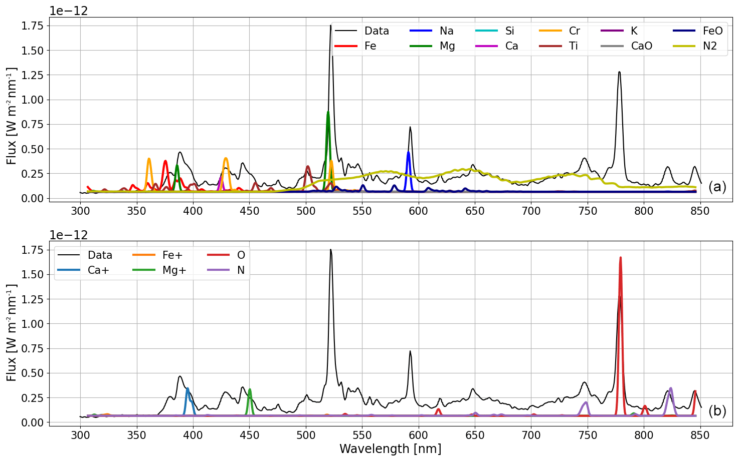
Figure 10 Same as Fig. 9, with (a) showing the synthetic spectra of all chemical elements analyzed for the meteor event for the lower-temperature component and (b) showing the synthetic spectra of all chemical elements analyzed for the meteor event for the higher-temperature component. From Fig. 7 one can find that the lower- and higher-temperature components resulting from the Bayesian method were 4000 and 9000 K, respectively.

For validation purposes the archive contains a subdirectory named “plots”, containing for each meteor event three different images in PNG format:

• eventname_lev3_fit.png, a plot of the observed spectrum overlaid with the synthetic spectrum – see Fig. 9;

• eventname_lev3_elementsfit.png, containing two plots of the observed spectrum, with the synthetic spectra of each chemical element overlaid (see Fig. 10); and

• eventname_lev3_chain.png, containing the MCMC chain results from each chemical element used in the PARADE simulation – see Sect. 7.1 and Fig. 7.

10 Summary

We present an algorithm to process meteor events acquired using a camera system with a spectral grating attached to it from raw format into quantitative chemical information. The algorithm is based on the principle that the location of a specific diffracted wavelength in first order can be directly derived from the knowledge of the zero-order position of the meteor. In our setup, we obtain the zero-order information from an image-intensified camera that is mounted with an offset angle to another intensified camera with a transmission grating mounted on top. The presented algorithm includes the radiometric calibration of the images, the determination of the location of the first-order information for each wavelength, the extraction of the meteor event spectral profile, and its spectral calibration. The spectrum derived is further corrected for atmospheric effects that take place between the observer and the location of the meteor ablation at the different heights during the event. In the next step, a Bayesian approach is used to map a simulated spectrum against the reduced spectrum obtained by our algorithm. To simulate the ablation we use the PARADE tool that was extended to allow the simulation for most meteoric and atmospheric atoms, diatomic molecules, ions, oxides, and a few complex molecules. As pre-knowledge for the Bayesian framework we use the assumption of two main temperature regimes during the ablation, as well as the typical chemical elements of meteors and their respective line intensities. After running typically 1000 Markov chain Monte Carlo iterations, we obtain the simulated spectrum as overall line intensities, but also obtain the line intensities of each chemical element. In a last processing step, the line intensities are calibrated themselves, resulting in the number densities of each chemical element.

Several hundred meteor events have been observed by CILBO in the past decade, and we provide full access to the data at their raw and intermediate calibrated data processing levels. The data are stored using the FITS standard, and an overview of the keyword–value pairs in the FITS header, as well as a description of the extended binary arrays used in the FITS extensions, is provided.

A discussion of one meteor event, its processing chain, and resulting spectral information is given.

The presented algorithm works autonomously – that means without user interaction. The processing time is, however, large, and even when using a multi-processor, multi-core system, we have not yet computed all individual frames of all meteor events. Instead, we have processed for each meteor event the information obtained from the total image as well as from the brightest frame. In the dataset published, we share the data representing the total image.

All events contained in the dataset have been checked for the convergence of the Bayesian parameters as a result of the MCMC iterations. The list of chemical elements used in the Bayesian approach was not extensive, and in the processing so far, we only checked for the typical chemical elements also reported by other observers in the past. It is our goal to reprocess all the data and use more chemical elements than PARADE is currently able to simulate. Such a step, however, needs a very careful study of the convergence of the chemical elements – which is still a manual step thus requiring dedicated efforts.