the Creative Commons Attribution 4.0 License.
the Creative Commons Attribution 4.0 License.
 | 26 Jun 2024
Airborne electromagnetic data levelling based on the structured variational method
Qiong Zhang
Xin Chen
Zhonghang Ji
Fei Yan
Zhengkun Jin
Yunqing Liu
Levelling errors are defined as the data difference among flight lines in airborne geophysical data. The differences in the signal levelling always appear as a striping pattern parallel to the flight lines on the imaged maps. The fixed structured pattern inspires us to structure a guided levelling error model using an anisotropic Gabor filter. We then embed the levelling error model into a total variational framework to flexibly calculate levelling errors. The guided levelling error model constrains the noise term of total variation rather than just using blind removal. Moreover, we can also apply the structured variational method to remove other noises in airborne geophysical data. This would just require replacing the noise prior models in the proposed method. We have applied this method to the airborne electromagnetic, magnetic, and apparent conductivity data collected by the Ontario Geological Survey to confirm its validity and robustness by comparing the results with the published data. The structured variational method can better level the airborne geophysical data based on the space properties of the levelling error.
- Article
(7299 KB) - Full-text XML
- Companion paper
- BibTeX
- EndNote


Airborne geophysical exploration is performed on an aircraft that moves at a high speed and at a certain elevation. The dynamic measuring mode brings convenience and efficiency but also constantly changes with the surrounding environment of the aircraft (Luyendyk, 1997; Gao et al., 2021). The aircraft data are acquired under different flight conditions and have unequal data levels that are defined as levelling errors. Levelling errors show up as a striping pattern along the flight direction because of the continuous “S-type” flight mode (Hood, 2007).
The airborne geophysical survey is commonly carried out in a long-term and large-scale measurement. Mathematically, a variety of factors contribute to the levelling errors, which are described as a distributed parameter model. The uncontrollable external environment is the main source of the levelling errors in an airborne geophysical survey. The seasonal and regional climate brings with it temperature fluctuations and natural wind changes. The temperature influences the internal aircraft configuration, and the wind directly changes the external inclination angle of the aircraft (Huang and Fraser, 1999; Valleau, 2000; Siemon, 2009). This leads to the conclusion that the external environment cannot be deemed to be a lumped parameter model and indirectly affects the data levels of each survey point.
Other factors are related to the intrinsic property of airborne measuring. Airborne surveys routinely fly in a continuous “S-type” flight mode at certain elevations. When the aircraft changes direction, the left and right sides of the aircraft alternately face the same surrounding environments. The opposite direction between adjacent lines causes the minor difference in flight attitude angle and other system configurations (Yin and Fraser, 2004; Huang, 2008). In addition, it is impossible to keep a constant flying altitude, no matter how advanced the flight systems are and how much experience the personnel operating them have (Tezkan et al., 2011; Eppelbaum and Mishne, 2011). The minor fluctuation factors that contribute to levelling errors are hard to control and measure.
The sources of the levelling errors are multiplicative and unable to quantitatively describe. It is hard to set up mechanism modelling of levelling errors. Currently, geophysicists base on the definition of levelling error and carry out data processing.
1.1 Tie line levelling method
A traditional but effective method is tie line levelling. Comparing the flight line data with tie line data at the same survey point, the operators correct the crossover point based on the differences between the tie lines and flight lines. The accuracy of tie line levelling mainly relies on whether the differences match the levelling errors. Many geophysicists have proposed algorithms to improve matching precision (Foster et al., 1970; Yarger et al., 1978; Bandy et al., 1990; Mauring et al., 2002; Srimanee et al., 2020). However, the flight line data and the tie line data are flown in different aircraft configurations and external environments. Moreover, airborne electromagnetic data are relatively sensitive to altitude compared with airborne magnetic data. The levelling error is not the only reason for the accumulation of the differences in the crossover point. It is hard to separate the levelling errors from the differences. Furthermore, virtual tie lines (Huang and Fraser, 1999; Fan et al., 2016; Zhang et al., 2018) are skilfully constructed to level geophysical data instead of tie lines.
1.2 Block levelling method
From the definition of levelling error, the inconsistent data level in flight lines is attributed to levelling errors that are not continuous between adjacent flight lines. However, as survey area geology changes quite slowly, it is reasonable to assume that the natural survey points are correlated in a certain region. The levelling errors can then be derived from line to line based on the differences between adjacent flight lines (Green, 2003; Huang, 2008; Zhu et al., 2020). Moreover, geophysicists skilfully constructed one-dimensional (1D) flight line windows and two-dimensional (2D) planar windows, considering the statistical parameters difference between the flight line data and region data. The levelling errors are calculated from point to point by matching the difference between the 1D and 2D window values (Mauring and Kihle, 2006; Beiki et al., 2010; Ishihara, 2015). Moreover, the geophysical data can be micro-levelled using the statistical approach in a designated moving window (Davydenko and Grayver, 2014; Groune et al., 2018).
1.3 Global levelling method
The line-to-line and point-to-point methods only level small amounts of data in each loop that can be deemed as block processing methods. A common problem is cumulative inaccuracies that develop when the levelled data are used to level in the next loop. In contrast, global processing methods operate the entire region data instead of only part data in every iteration. The global processing methods available mainly focus on airborne magnetic data levelling based on the separated long-wavelength components (Urquhart, 1988; Nelson, 1994; Luo et al., 2012; White and Beamish, 2015; Zhang et al., 2021). The directional filters are designed to level the geophysical data (Minty, 1991; Ferraccioli et al., 1998; Siemon, 2009; Gao et al., 2021).
In summary, the conventional block processing methods would inevitably transfer errors. The global processing methods mainly focus on levelling airborne magnetic data. As with the levelling error properties discussed above, the levelling error is an additive drift, presented as the inconsistent data level among the flight lines. These inconsistencies are affected by a variety of factors that make it hard to construct a mechanism model for levelling errors. However, the striping errors would increase the total variation of the measuring area. Total variational theory inspires us to level the data by using an energy functional model. The proposed method is described below.
During the survey area space analysis, levelling errors are formed along the flight lines and have definitive directional distribution properties (Zhang et al., 2022). The directional stripes would further cause discontinuities in the vertical direction and increase the horizontal gradient amplitude. The total variational model can detect and remove all the components that impair the total smoothness. While we specifically focus on levelling errors, a detailed constraint is helpful. Thus, we build a levelling error model based on the prior information and properly embed the model in the total variational model. In the proposed method, only the levelling errors are extracted and removed through solving the constrained and structured variational model.
2.1 Total variational model
The theoretical basis of most levelling techniques is that the geophysical field is continuous. The observed data tend to show significant correlations with their neighbouring points. However, the levelling errors are not continuous between adjacent flight lines (Huang, 2008). When the assumption is valid, the geophysical data with levelling errors will have a large variation amplitude compared with nature geophysical data. It is thus advisable to estimate the levelling error components based on total variation model.
We simply deemed the survey data consists of two parts:
where S(i,j) is the ith survey data in the jth flight line, E(i,j) is the levelling error component of the survey point, and D(i,j) is the levelled data. Here the survey data are considered a 2D function in the entire region Ω, while (i,j) defines the ith survey data in the jth flight line.
Rudin et al. (1992) introduced total variation norm and proposed Rudin–Osher–Fatemi (ROF) total variation model, which has been widely used in image-denoising applications. Based on total variational model, we can estimate the levelling error components by constructing an energy functional,
where λ is the regularisation coefficient that quantifies the degree of smoothness. Based on the multiscale hierarchical decomposition theory (Tadmor et al., 2003), we can determine the regularisation coefficient by the spatially adaptive multi-scale model (Zhang et al., 2022). TV(D) is the total variation of the estimated solution D expressed as follows:
In the total variational model, is a fidelity term which ensures the similarity between the original data S and the clear data D. In Eq. (2), L−2 norm is selected to build the fidelity term due to its excellent edge-preserving performance.
TV(D) serves as the regularisation term, aimed at penalising undesirable damage in data. The regularisation term is the total variation of the estimated solution. It means that sparse gradient domain constraints are imposed along the horizontal and vertical directions. Combined with prior information, the levelling error components can be computed by minimising the total variation model in Eq. (2). The total variational model has been applied to the striping noise removal (Zhang and Zhang, 2016; Liu et al., 2019).
2.2 Levelling error model
Accurately extracting levelling errors requires us to combine the total variation model with as much prior information about the levelling error as possible. Levelling errors present a significant directional property and show up as a striping pattern along the flight direction. We can the design an anisotropic Gabor filter with the principal axis directed by the levelling error.
In geophysical exploration, the levelling error model should estimate the intensity at each survey point, which can be modelled as follows:
where α is the weight coefficient that describes the intensities of levelling error, while G is the noise pattern. We model stripes as an anisotropic Gaussian function defined by
In Eq. (5), (i,j) defines the location of the ith survey data in the jth flight line. θ represents the normal's orientation to the Gabor function's parallel stripes, that is, the flight line direction. σi and σj are the Gaussian envelope's standard deviation in the x direction and flight line direction, respectively.
The pattern of levelling error is mainly described by the Gaussian function. We can obtain the parameters in Eq. (5) combined with prior shape information. The weight coefficient defines the levelling error intensity that is necessary to solve from the overall view.
2.3 Structured variational model
When we guide the total variational model levelling by levelling error model, the structured variational model provides an accurate geophysical processing design. We obtain the following objective function:
Equation (6) contains two coefficients, α and λ, to balance the fidelity term and regularisation term. It is permitted to reasonably merge the two coefficients and express Eq. (6) as follows:
We then use alternating direction method of multipliers (ADMM) to solve non-convex optimisation problems. ADMM converts the original problem into subproblems with closed-form solutions. It is an effective approach in a sequence of iterative sub-optimisations (Bertsekas, 1982).
While the levelling error intensity for each survey point is solved, we complete the data levelling using Eqs. (1) and (4) under the structured variational model.
In exploration field, airborne geophysical measurement data contains a large amount of noise due to atmospheric flow, lightning, aircraft vibration, and unstable speed factors (Yin et al., 2015). In addition to levelling errors, different kinds of noises damage the measurement data simultaneously. Here, we simply assume the measurement data contains levelling errors and Gaussian white noise. In that case, the proposed levelling method has an obvious advantage compared with other levelling methods. The proposed method constructs an energy functional as Eq. (2). For other noise, we can consider the denoising problem under the framework similarly. The noise model in Eq. (4) describes the noise distribution and geometrical structure. When we try to remove several kinds of several kinds of disturbances, Eq. (4) is extended as follows:
where n is the number of noise type.
For Gaussian white noise, it can be obtained by convolving a Dirac function with a sample of white Gaussian noise. The proposed method simultaneously removes the levelling errors and Gaussian white noise in one step processing that helps to improve electromagnetic exploration accuracy.
Thus, there are three evident advantages in proposed levelling method.
-
The total variation model designs the total energy as a constraint condition and obtains the constrained gradient minimisation using the regularisation coefficient. When we use total variational model to deal with survey area data, it can reasonably remove the levelling errors that increase the gradient of survey area data.
-
Due to the complexity of airborne geophysical field measurement, there are multiple components in airborne geophysical data. To focus on levelling error extraction, we construct a rough levelling error model based on the striping pattern. The levelling error model is then embedded into the gradient minimisation functional and clearly solved in the structured variational model.
-
The structured variational model can be carried over into other noise. If it accesses the noise characteristic and establishes the noise model, we can speculate that the structured variational model can remove other noises. The framework may take effect based on the precise noise model.
We have verified these advantages through experimentation.
3.1 Airborne magnetic data levelling
3.1.1 Real dataset example
The levelling method has been tested on magnetic field data obtained by Geotech Limited. Figure 1 shows the magnetic data before and after levelling. The survey area data include 117 flight lines with a line spacing of 200 m and contain striped levelling errors along flight line direction. In the example, we only focus on levelling errors in Fig. 1a. The noise pattern in Eq. (5) is set based on the prior information about levelling errors. For example, we set the normal orientation θ as 90° because the flight line direction is vertical in the general coordinate system. The Gaussian envelope's standard deviation σi and σj decide the number of stripes. The ratio of σi and σj represents the spatial shape of the Gabor function. When we use the Gabor function to describe levelling errors, should be much lower than 1. Figure 1b shows the data processed by the proposed levelling method, while Fig. 1c presents the data levelled by the classic tie line levelling method.
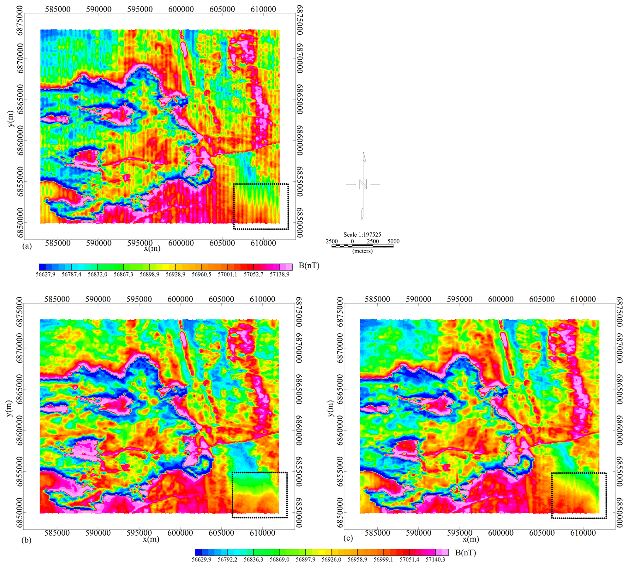
Figure 1Airborne magnetic data levelling. (a) Raw magnetic data. (b) Levelling results using the proposed levelling method. (c) Levelling results using the tie line levelling method.
3.1.2 Synthetic dataset example
The example is from a synthetic magnetic dataset with additional Gaussian white noise and levelling errors. We selected the levelling results that used the tie line levelling method as the clean data. The data have been explained in the real dataset example and are presented in Fig. 1c. We then tested our algorithm on the noisy magnetic data as shown in Figs. 2 and 3. There are three experiments, including specific clean data with Gaussian white noises, clean data with levelling errors, and clean data with Gaussian white noises and levelling errors.
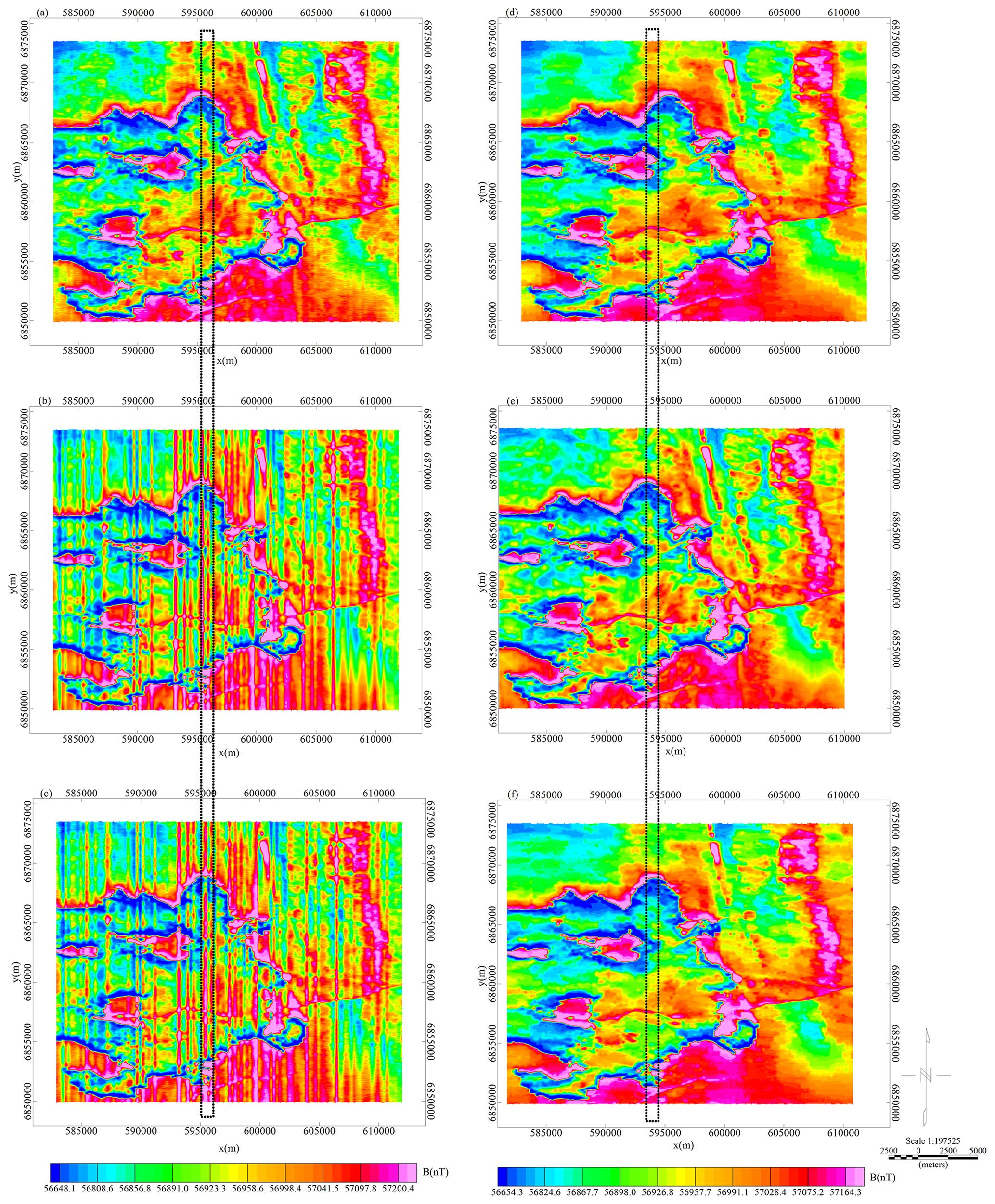
Figure 2Synthetic airborne magnetic data processing. (a) Magnetic data with Gaussian white noise. (b) Magnetic data with levelling errors. (c) Magnetic data with Gaussian white noise and levelling errors. (d) Denoised results of (a) data. (e) Denoised results of (b) data. (f) Denoised results of (c) data. Panels (a)–(c) have been adjusted to use the same colour bar. Panels (d)–(f) have been adjusted to use the same colour bar.
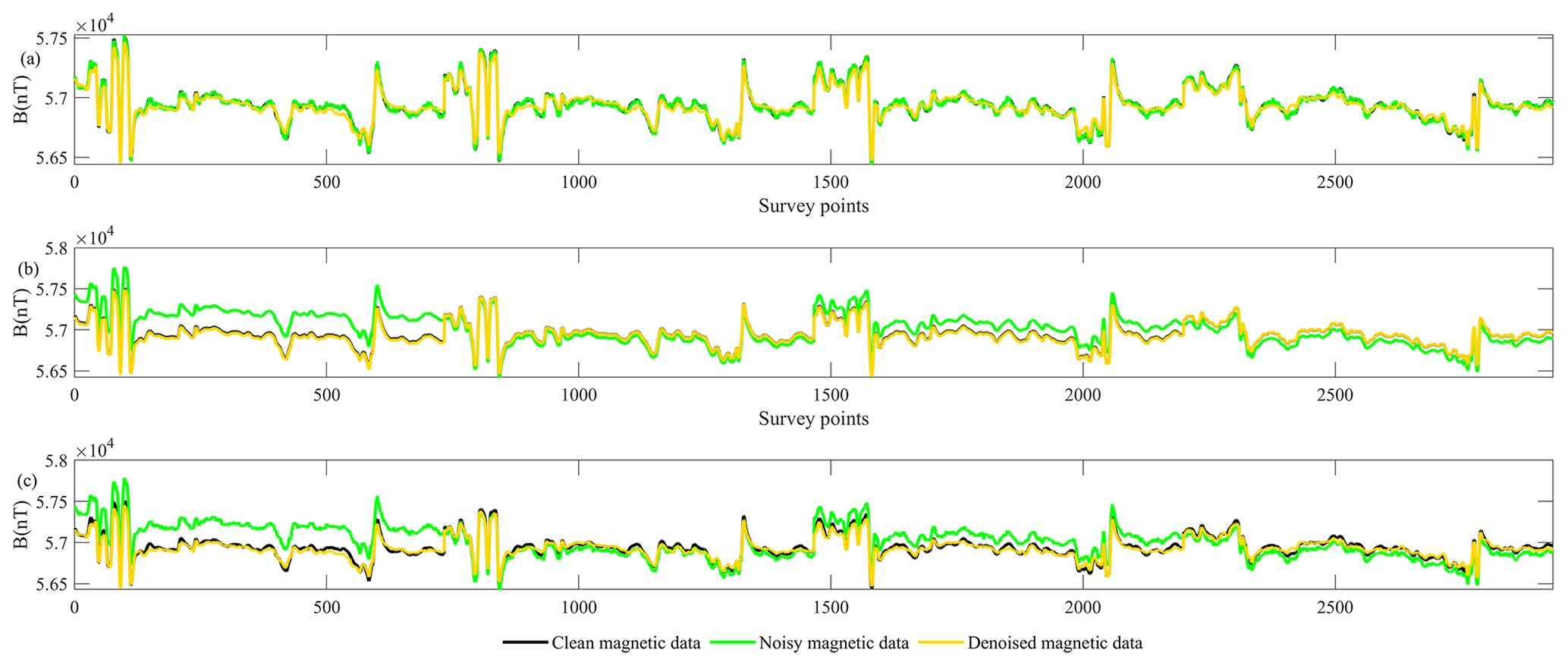
Figure 3Levelling result analysis of synthetic airborne magnetic data. (a) Magnetic data with Gaussian white noises. (b) Magnetic data with levelling errors. (c) Magnetic data with Gaussian white noises and levelling errors.
The first synthetic dataset focuses on removing Gaussian white noises. We are required to estimate and obtain the noise model using the white noise estimation method. The structured variational model will then be guided to remove the corresponding noise type. Figure 2a and d show the data before and after processing. The second synthetic dataset focuses on removing levelling errors. Figure 2b is the clean data with levelling errors. We use a Gabor filter to simulate the levelling error model, and Fig. 2e shows the data after processing. The third synthetic dataset is designed with two noise components as shown in Fig. 2c. While the proposed method intends to remove the noises simultaneously, the noise model in Eq. (8) must include the Gaussian white noise model and levelling error model. The proposed method then removes the two noise sources via an objective function. Figure 2c and f shows the noisy magnetic data before and after processing.
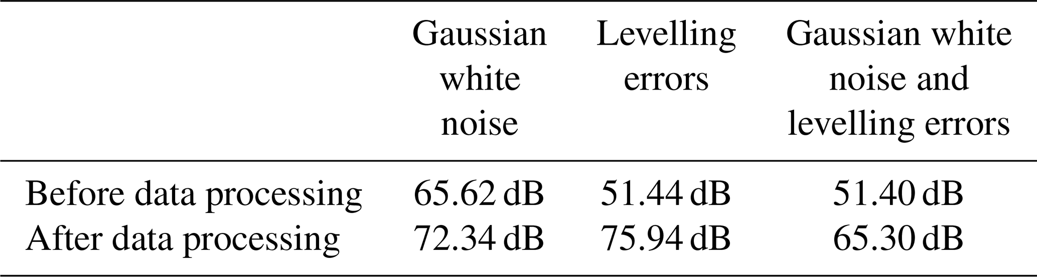
Furthermore, we calculated the signal-to-noise ratio (SNR) for the three experiments. The quantitative comparison is shown in Table 1, and Fig. 3 illustrates the transient data to compare the results in greater detail. There are four flight lines that have been locally enlarged, corresponding to the dotted black rectangle in Fig. 2. The three subgraphs separately analysed the three experiments above. In every subgraph, the blue curve represents the clean magnetic data, the red curve represents the noisy magnetic data, and the green curve represents the denoised magnetic data.
3.2 Apparent conductivity data levelling
We also tested the levelling method on the apparent conductivity data provided by Ontario Airborne Geophysical Surveys. The dataset used in the paper is formed by 70 flight lines named L310–L1000 as a part of Geophysical Data Set 1076 measured in the surveys (Ontario Geological Survey, 2014). Geotech Limited carried out a helicopter-borne combined aeromagnetic and electromagnetic survey for the Ministry of Northern Development and Mines in 2014 in the Nestor Falls area in northwestern Ontario. Based on the resistivity depth imaging (RDI) technique (Meju, 1998), Geotech Limited converted the EM profile decay data into an equivalent resistivity versus depth cross-section via deconvolution of the measured TEM data. Data compilation and processing were carried out using Geosoft® OASIS montajTM and programs proprietary to Geotech Ltd (Ontario Geological Survey 2014).
Figure 4 presents the apparent conductivity data before and after levelling processing. As Fig. 4a shows, there are only slight striped errors along the flight line direction in the apparent conductivity data. While the electromagnetic data are transformed into conductivity parameters, the altitude sensitivity is strongly weakened (Fraser, 1972; Huang and Fraser, 1999).
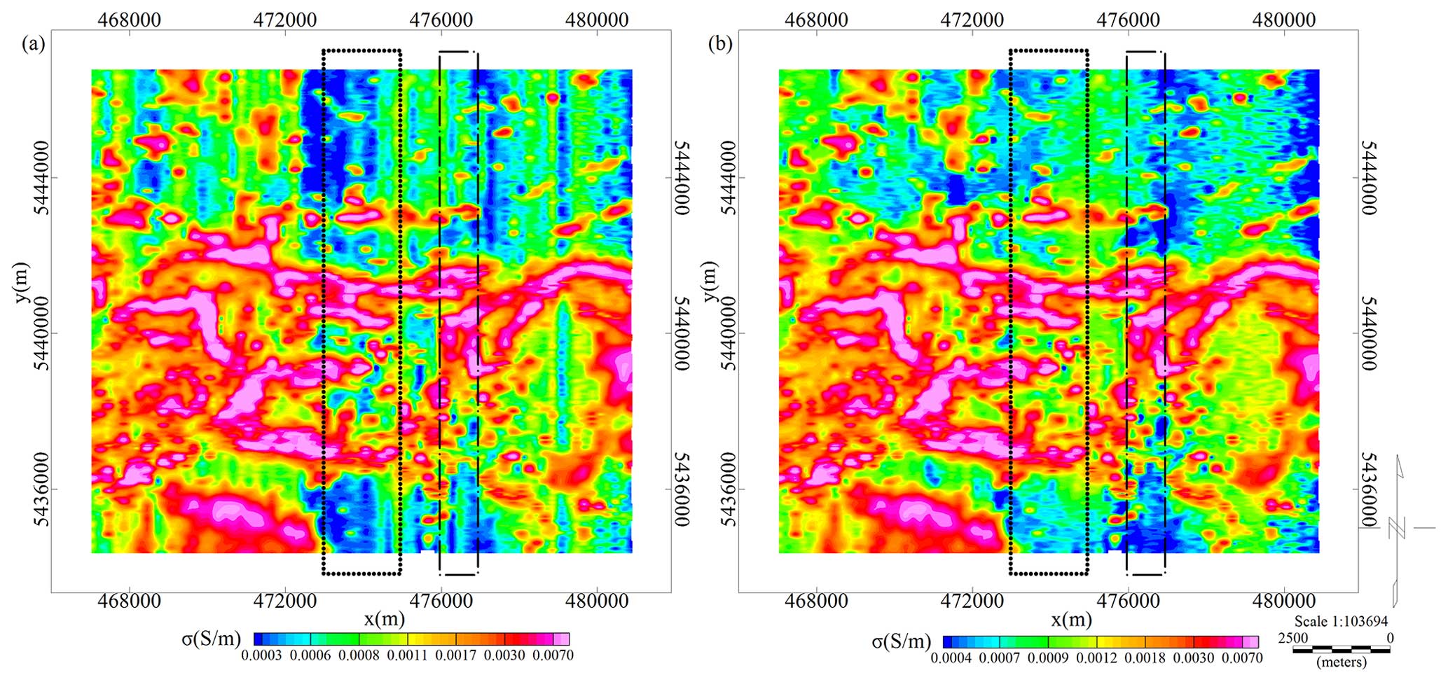
Figure 4The levelling of the apparent conductivity data. (a) The raw data. (b) Levelling results using the proposed levelling method.
We then applied the structured variational model to the apparent conductivity data and got the levelling results as Fig. 4b shown. In the analysis of the data, it is assumed that the levelling error is the only noise source. Figure 5 illustrates the transient data to compare the results in greater detail. Two parts of the data are plotted corresponding to the black rectangle in Fig. 4. The first part includes 10 flight line datasets as shown in Fig. 5a. We then selected a smaller data scope (0– S m−1) to locally enlarge and draw the data in Fig. 5b. Figure 5c and d are drawn using the five flight line dataset that are correspond to the dashed–dotted black rectangle in Fig. 4.
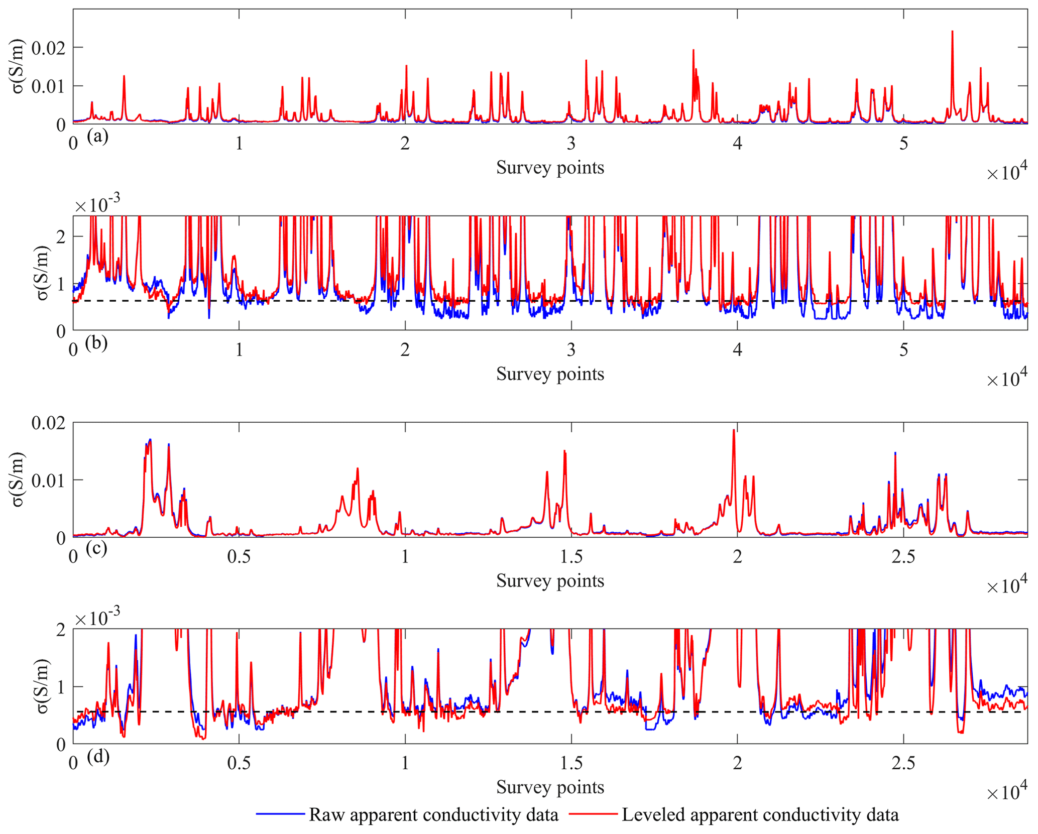
Figure 5Levelled apparent conductivity data. (a) The 10 flight line datasets, corresponding to the dotted black rectangle in Fig. 4. (b) Local enlarged curves of (a) data. (c) The five flight line datasets, corresponding to the dashed–dotted black rectangle in Fig. 4. (d) Local enlarged curves of the data in (c).
Firstly, we analysed and discussed the levelling results in an airborne magnetic data example in Fig. 1. As seen in Fig. 1b and c, most of the striped levelling errors have been removed using the proposed levelling method and tie line levelling method. A careful contrast of the two results shows that tie line levelling method leaves some weak levelling errors that are clear in the dotted black rectangle in Fig. 1.
The residue in the tie line levelling method may be caused by an incompatible data alignment. Although the levelling errors show a striped pattern in the survey area map, they are slowly changing from point to point in a certain flight line. The tie line levelling method adjusts the flight line data to match the tie line data. Because the tie line number is much lower than the point survey number, it needs to build a model using the crossover point differences of the tie lines and flight lines. When only a few tie line data points are used to calculate the levelling error of every point, it is hard to balance every point using an exact model.
In this paper we proposed a new technology based on the ROF total variation model that focuses on the gradient change in measured data. As the basic principle of data levelling, theoretical geophysical data have continuous change regularities. Levelling errors break the continuity and increase the total variation of the survey area data (Zhang et al., 2022). In the proposed levelling method, the structured variational model aims to minimise the energy functional to better explore the levelling errors in the data.
We then evaluated a synthetic magnetic example to further analyse the results. There are three experiments with different noises: (1) Gaussian white noise, (2) levelling errors, and (3) mixed noise with Gaussian white noise and levelling errors. As shown in Fig. 2, the structured variational model can visibly remove the noise. In theory, noise increases the gradient amplitude. The proposed model can be robust for smoothing the gradient of the survey area data in an energy functional.
There is a transient data comparison in Fig. 3. In the three experiments, the results of the transient data (yellow lines) are very similar to the clean data (black lines). The data processing is without the localised anomalies being trimmed. Three groups of SNRs are calculated in Table 1. The robustness of the proposed model means it can deal with different noise type. A suitable noise model still needs to be set, otherwise it may lead to over-smoothing effect.
Finally, we test the levelling method on apparent conductivity data. Compared with Figs. 1a and 4a, apparent conductivity as a response domain is slightly affected by levelling errors. However, the differences in data levels still interfere data interpretation. Figure 5 can better evaluate how well the method is working. We deem the bottom of data curve to represent the data level and enlarge the small data scope as shown in Fig. 5b and d, and a dashed black line is added as a measured rule. The blue lines in Fig. 5 are the apparent conductivity data without levelling. It is obvious that the bottom of blue lines hover around the dashed black lines in Fig. 5b and d. When we adjusted the data, the data levels are united as the red lines show in Fig. 5. The slight levelling errors are tested and removed by the proposed levelling method. The method is effective to time-domain airborne electromagnetic data and response-domain airborne electromagnetic data.
In this paper, we proposed a levelling method based on a structured variational method. The basis of this method is that levelling errors increase the gradient of survey area data. The ROF total variation model has been proposed by Rudin et al. (1992) and designed with the total energy as a constraint condition. Moreover, it shows potentially good performance in smoothing the total gradient by minimising the constrained gradient. The regularisation coefficient plays a role in controlling the smoothness. The ROF total variation model can adjust the airborne electromagnetic data by smoothing the total gradient.
A rough levelling error model is constructed to focus on levelling error accurately. Based on the levelling error characteristic, we introduced the Gabor filter to match the levelling error with the striping pattern. Furthermore, the rough levelling error model is embedded into the ROF total variation model to construct a structured variational model. The proposed model is guided to deal with the additional gradient caused by levelling errors. We have confirmed the method's reliability by applying it to the magnetic, synthetic magnetic, and apparent conductivity data.
In addition, the synthetic magnetic example has tested the structured variational model, which can also handle other noise. A suitable noise model still needs to be embedded into the ROF total variation model. Otherwise, it may lead to an over-smoothing effect and loss of accuracy.
The data used in the paper have been opened by Ontario Geological Survey. More information can be found at their official website (https://www.hub.geologyontario.mines.gov.on.ca/, Zhang et al., 2022).
The manuscript was approved by all authors for publication. QZ and XC developed the algorithm model and performed the simulations. ZJi designed the experiments. ZJin and FY carried them out. YL prepared the manuscript with contributions from all co-authors.
The contact author has declared that none of the authors has any competing interests.
Publisher's note: Copernicus Publications remains neutral with regard to jurisdictional claims made in the text, published maps, institutional affiliations, or any other geographical representation in this paper. While Copernicus Publications makes every effort to include appropriate place names, the final responsibility lies with the authors.
We all thank the Ontario Geological Survey for giving us permission to use the geophysical data featured in this study. Moreover, the authors are appreciative of Jean M. Legault, Chief Geophysicist of Geotech Ltd, for providing us with access to Geophysical Data Set 1076. We also appreciate the editors and reviewers very much for their positive and constructive comments and suggestions that improved our manuscript.
This research has been supported by the National Natural Science Foundation of China (grant no. 42204144).
This paper was edited by Lev Eppelbaum and reviewed by Rudi Cop and one anonymous referee.
Bandy, W. L., Gangi, A. F., and Morgan, F. D.: Direct method for determining constant corrections to geophysical survey lines for reducing mis-tie, Geophysics, 55, 885–896, https://doi.org/10.1190/1.1442903, 1990.
Beiki, M., Bastani, M., and Pedersen, L. B.: Leveling HEM and aeromagnetic data using differential polynomial fitting, Geophysics, 75, 13–23, https://doi.org/10.1190/1.3279792, 2010.
Bertsekas, D. P.: Constrained optimization and Lagrange Multiplier methods, Computer Science and Applied Mathematics, Academic Press, Boston, MA, USA, ISBN 1886529043, 1982.
Davydenko, A. Y. and Grayver, A. V.: Principal component analysis for filtering and leveling of geophysical data, J. Appl. Geophys., 109, 266–280, https://doi.org/10.1016/j.jappgeo.2014.08.006, 2014.
Eppelbaum, L. V. and Mishne, A. R.: Unmanned Airborne Magnetic and VLF investigations: Effective Geophysical Methodology of the Near Future, Positioning, 2, 112–133, https://doi.org/10.4236/pos.2011.23012, 2011.
Fan, Z. F., Huang, L., Zhang, X. J., and Fang, G. Y.: An elaborately designed virtual frame to level aeromagnetic data, IEEE Geosci. Remote Sens. Lett., 13, 1153–1157, https://doi.org/10.1109/LGRS.2016.2574750, 2016.
Ferraccioli, F., Gambetta, M., and Bozzo, E.: Microlevelling procedures applied to regional aeromagnetic data: an example from the Transantarctic Mountains, Geophys. Prospect., 46, 177–196, https://doi.org/10.1046/j.1365-2478.1998.00080.x, 1998.
Foster, M. R., Jines, W. R., and Weg, K. V.: Statistical estimation of systematic errors at intersections of lines of aeromagnetic survey data, J. Geophys. Res., 75, 1507–1511, https://doi.org/10.1029/JB075i008p01507, 1970.
Fraser, D. C.: A new multicoil aerial electromagnetic prospecting system, Geophysics, 37, 518–537, https://doi.org/10.1190/1.1440277, 1972.
Gao, L. Q., Yin, C. C., Wang, N., Liu, Y. H., Su, Y., and Xiong, B.: Leveling of airborne electromagnetic data based on curvelet transform, Chinese J. Geophys., 5, 1785–1796, https://doi.org/10.6038/cjg2020N0365, 2021.
Green, A.: Correcting drift errors in HEM data, ASEG Spec. Publ., 2, 1, https://doi.org/10.1071/aseg2003ab058, 2003.
Groune, D., Allek, K., and Bouguern, A.: Statistical approach for microleveling of aerophysical data, J. Appl. Geophys., 159, 418–428, https://doi.org/10.1016/j.jappgeo.2018.09.023, 2018.
Hood, P.: History of Aeromagnetic Survey in Canada, Leading Edge, 26, 1384–1392, https://doi.org/10.1190/1.2805759, 2007.
Huang, H. P.: Airborne geophysical data leveling based on line-to-line correlations, Geophysics, 73, 83–89, https://doi.org/10.1190/1.2836674, 2008.
Huang, H. P. and Fraser, D. C.: Airborne resistivity data leveling, Geophysics, 64, 378–385, https://doi.org/10.1190/1.1444542, 1999.
Ishihara, T.: A new leveling method without the direct use of crossover data and its application in marine magnetic surveys, weighted spatial averaging and temporal filtering, Earth Planets Space, 67, 1–14, https://doi.org/10.1186/s40623-015-0181-7, 2015.
Liu, L., Xu, L. P., and Fang, H. Z.: Simultaneous Intensity Bias Estimation and Stripe Noise Removal in Infrared Images Using the Global and Local Sparsity Constraints, IEEE T. Geosci. Remote, 58, 1777–1789, https://doi.org/10.1109/TGRS.2019.2948601, 2019.
Luo, Y., Wand, P., Duan, S. L., and Cheng, H. D.: Leveling total field aeromagnetic data with measured vertical gradient, Chinese J. Geophys., 55, 3854–3861, https://doi.org/10.6038/j.issn.0001-5733.2012.11.033, 2012.
Luyendyk, A. P. J.: Processing of airborne magnetic data, AGSO J. Aust. Geol. Geophys., 17, 31–38, 1997.
Mauring E. and Kihle, O.: Leveling aerogeophysical data using a moving differential median filter, Geophysics, 71, 5–11, https://doi.org/10.1190/1.2163912, 2006.
Mauring, E., Beard, L. P., and Kihle, O.: A comparison of aeromagnetic levelling techniques with an introduction to median leveling, Geophys. Prospect., 50, 43–54, https://doi.org/10.1046/j.1365-2478.2002.00300.x, 2002.
Meju, M. A.: Short Note: A simple method of transient electromagnetic data analysis, Geophysics, 63, 405–410, https://doi.org/10.1190/1.1444340, 1998.
Minty, B. R. S.: Simple micro-levelling for aeromagnetic data, Explor. Geophys., 22, 591–592, https://doi.org/10.1071/eg991591, 1991.
Nelson, J. B.: Leveling total-field aeromagnetic data with measured horizontal gradients, Geophysics, 59, 1166–1170, https://doi.org/10.1190/1.1443673, 1994.
Ontario Geological Survey: Ontario airborne geophysical surveys, magnetic and electromagnetic data, grid and profile data (ASCII and Geosoft® formats) and vector data, Nestor Falls area, Geophysical Data Set 1076, Ontario Geological Survey, 2014.
Rudin, L. I., Osher, S., and Fatemi, E.: Nonlinear total variation based noise removal algorithms, Physica D, 60, 259–268, https://doi.org/10.1016/0167-2789(92)90242-F, 1992.
Siemon, B.: Levelling of helicopter-borne frequency-domain electromagnetic data, J. Appl. Geophys., 67, 206–218, https://doi.org/10.1016/j.jappgeo.2007.11.001, 2009.
Srimanee, C., Dumrongchai, P., and Duangdee, N.: Airborne gravity data adjustment using a cross-over adjustment with constraints, Int. J. Geoinform., 16, 51–60, 2020.
Tadmor, E., Nezzar, S., and Vese, L.: A multiscale image representation using hierarchical, Multiscale Model. Simul., 2, 554–579, https://doi.org/10.1137/030600448, 2003.
Tezkan, B., Stoll, J. B., Bergers, R., and Grossbach, H.: Unmanned aircraft system proves itself as a geophysical measuring platform for aeromagnetic surveys, First Break, 29, 103–105, 2011.
Urquhart, T.: Decorrugation of enhanced magnetic field maps, Seg Technical Program Expanded Abstracts, SEG Library, 371–372, https://doi.org/10.1190/1.1892383, 1988.
Valleau, N. C.: HEM data processing – A practical overview, Explor. Geophys., 31, 584–594, https://doi.org/10.1071/eg00584, 2000.
White, J. C. and Beamish, D.: Levelling aeromagnetic survey data without the need for tie-lines, Geophys. Prospect., 63, 451–460, https://doi.org/10.1111/1365-2478.12198, 2015.
Yarger, H. L., Robertson, R. R., and Wentland, R. L.: Diurnal drift removal from aeromagnetic data using least squares, Geophysics, 43, 1148–1156, https://doi.org/10.1190/1.1440884, 1978.
Yin, C. C. and Fraser, D. C.: Attitude corrections of helicopter EM data using a superposed dipole model, Geophysics, 69, 431–439, https://doi.org/10.1190/1.1707063, 2004.
Yin, C. C., Ren, X. Y., Liu, Y. H., and Cai, J.: Exploration capability of airborne TEM systems for typical targets in the subsurface, Chinese J. Geophys., 58, 3370–3379, https://doi.org/10.6038/cjg20150929, 2015.
Zhang, Q., Peng, C., Lu, Y. M., Wang, H., and Zhu, K. G.: Airborne electromagnetic data levelling using principal component analysis based on flight line difference, J. Appl. Geophys., 151, 290–297, https://doi.org/10.1016/j.jappgeo.2018.02.023, 2018.
Zhang, Q., Yan, F., and Liu, Y. Q.: Airborne geophysical data levelling based on variational mode decomposition, Near Surf. Geophys., 19, 377–394, https://doi.org/10.1002/nsg.12138, 2021.
Zhang, Q., Sun, C., Yan, F., Lv, C., and Liu, Y.: Leveling airborne geophysical data using a unidirectional variational model, Geosci. Instrum. Method. Data Syst., 11, 183–194, https://doi.org/10.5194/gi-11-183-2022, 2022 (data available at: https://www.hub.geologyontario.mines.gov.on.ca/, last access: 1 February 2024).
Zhang, Y. Z. and Zhang, T. X.: Structure-guided unidirectional variation de-striping in the infrared bands of MODIS and hyperspectral images, Infrared Phys. Technol., 77, 132–143, https://doi.org/10.1016/j.infrared.2016.05.022, 2016.
Zhu, K. G., Zhang, Q., Peng, C., Wang, H., and Lu, Y. M.: Airborne electromagnetic data levelling based on inequality-constrained polynomial fitting, Explor. Geophys., 51, 600–608, 2020.