A tool for estimating ground-based InSAR acquisition characteristics prior to monitoring installation and survey and its differences from satellite InSAR

Synthetic Aperture Radar (SAR) acquisition can be performed from satellites or from the ground by means of a so-called GB-InSAR (Ground-Based Interferometry SAR), but the signal emission and the output image geometry slightly differ between the two acquisition modes. Those differences are rarely mentioned in the literature. This paper proposes to compare satellite and GB-InSAR in terms of (1) acquisition characteristics and parameters to consider; (2) SAR image resolution; and (3) geometric distortions that are foreshortening, layover, and shadowing.

If in the case of satellite SAR, the range and azimuth resolutions are known and constant along the orbit path, in the case of GB-InSAR their values are terrain-dependent. It is worth estimating the results of a GB-InSAR acquisition that one can expect in terms of range and azimuth resolution, line of sight (LoS) distance, and geometric distortions to select the best installation location when several are possible. We developed a novel tool which estimates those parameters from a digital elevation model (DEM), knowing the GB-InSAR and the slope of interest (SoI) coordinates. This tool, written in MATLAB, was tested on a simple synthetic point cloud representing a cliff with a progressive slope angle to highlight the influence of the SoI geometry on the acquisition characteristics and on two real cases of cliffs located in Switzerland, namely one in the Ticino canton and one in the Vaud canton.

1 Introduction

The use of Synthetic Aperture Radar Interferometry (InSAR) as a remote-sensing technique capable of detecting and monitoring small ground displacements started in the 1980s (Gabriel et al., 1989). It was initially used specifically with spaceborne platforms such as the satellites ERS-1 (1991) or RADARSAT (1995; Zebker and Villasenor, 1992; Massonnet et al., 1993; Usai and Hanssen, 1997). In the field of geosciences, this technique has been primarily dedicated to studying small movement phenomena (smaller than a few centimetres) across large areas (km) with a resolution ranging from decametric to metric scales, such as subsidence (Cabral-Cano et al., 2008; Strozzi et al., 2018), volcanic activities (Wicks et al., 1998; Garthwaite et al., 2019), or landslides (Tarchi, 2003; Hilley et al., 2004; Colesanti and Wasowski, 2006). Since then, the technique expanded, and by the late 1990s, the first radar devices monitoring displacements from a ground base (GB) were deployed (Cazzanil et al., 2000; Pieraccini and Miccinesi, 2019; Tarchi et al., 1997). Some use a Real Aperture Radar (RAR) antenna (Werner et al., 2008), while others employ a Synthetic Aperture Radar (SAR, Rudolf et al., 1999; Leva et al., 2003; Antonello et al., 2003).

InSAR satellites and GB-InSAR are complementary, with both detecting displacements only along their respective line of sight (LoS) (Casagli et al., 2003; Catani et al., 2014; Carlà et al., 2019). InSAR satellites detect sub-vertical movements, while GB-InSAR devices gather information on sub-horizontal movements (Wolff et al., 2023).

Radar image acquisition and processing are sensitive to terrain geometry, which can have significant effects on the appearance of the resulting radar image, such as slope compression and highlighting (foreshortening and layover effects) (Jensen, 2006) or surfaces not illuminated by the radar appearing dark and elongated in the image (shadowing effect). Terrain slopes and the radar incidence angle influence the image resolution. Satellite-imagery-oriented software creates foreshortening and layover masks (Kropatsch and Strobl, 1990; Rees, 2000). Although SAR satellite geometries are well documented (Griffiths, 1995; Rees, 2000; McCandless and Jackson, 2004; Ferretti et al., 2007), the transposition of these geometries to GB-InSAR is seldom mentioned in the literature. Nevertheless, before initiating a new GB-InSAR campaign, it is crucial to estimate what results one can expect in terms of the distance to the region of interest, range, and azimuthal resolutions, as well as potential foreshortening and shadowing effects, in order to select the best position before starting the campaign. This is particularly the case for the installation of a GB-InSAR in remote areas and difficult installation sites (Lingua et al., 2008; Caduff et al., 2015; Talich, 2016; Rouyet et al., 2017).

After transposing the SAR geometry described for satellites to ground SAR geometry and presenting the main differences between satellite and GB-InSAR, this paper describes a MATLAB tool with a user interface designed to compute several parameters of the radar image such as its range and azimuthal resolutions, as well as the areas affected by shadowing or strong foreshortening in the case of a linear SAR system consisting of a radar measuring head moving along a rail. The needed inputs are a digital elevation model (DEM) in an ASCII format, the localization of the area of interest, and the localization where one intends to install the GB-InSAR. The main objective is to provide a tool for helping surveyors to find the best installation location.

The tool has been tested across three study cases: (1) a synthetic cliff made of slope angles increasing from the bottom to the top and two real, unstable cliffs that have been monitored with a GB-InSAR at (2) Cima del Simano and (3) La Cornalle. For Cima del Simano, the results for three different radar positions were compared to select the best installation position.

2 Theory

2.1 SAR geometry

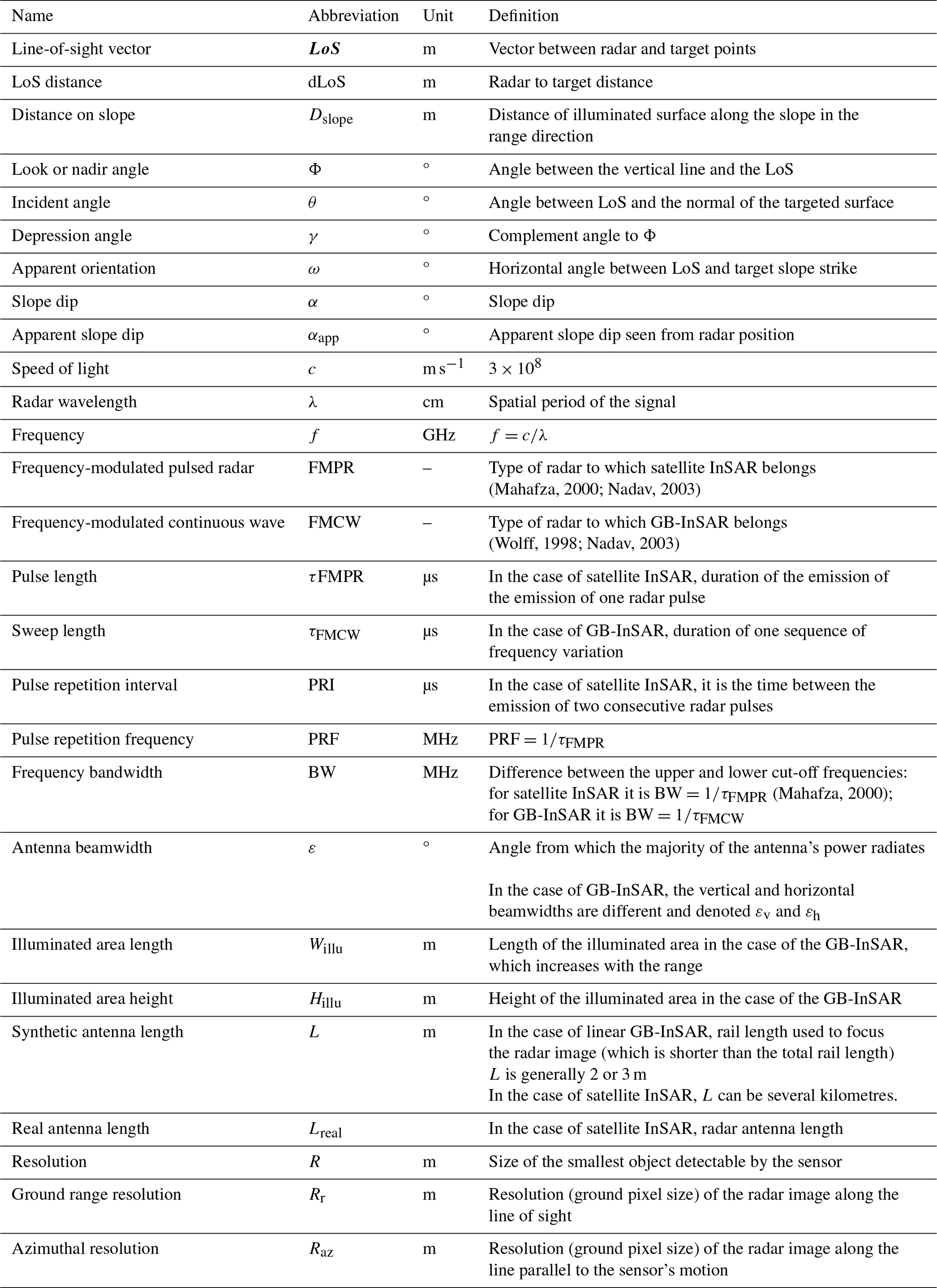
The geometrical characteristics of radar imagery differ from standard image geometry (Lin and Fuh, 1998; Turner et al., 2021). In the case of radar imagery, some parameters need to be defined and distinguished when applied to satellite and aerial InSAR or to GB-InSAR. The abbreviations are summarized in Table 1.

Table 1 List of abbreviations used for the radar characteristics presented hereafter.

2.1.1 LoS, azimuthal, and range directions

In the case of aerial radar, the azimuthal direction corresponds to the direction of the displacement of the aircraft or satellite; the range direction, or look direction, is the direction perpendicular to the azimuthal direction. The direction of the radar-to-target line is the LoS direction whose distance is called the range or LoS distance (dLoS). It varies from near-range, for the line forming the smaller angle with the vertical radar–Earth line (nadir), to the far-range for the direction with the larger angle (Fig. 1a).

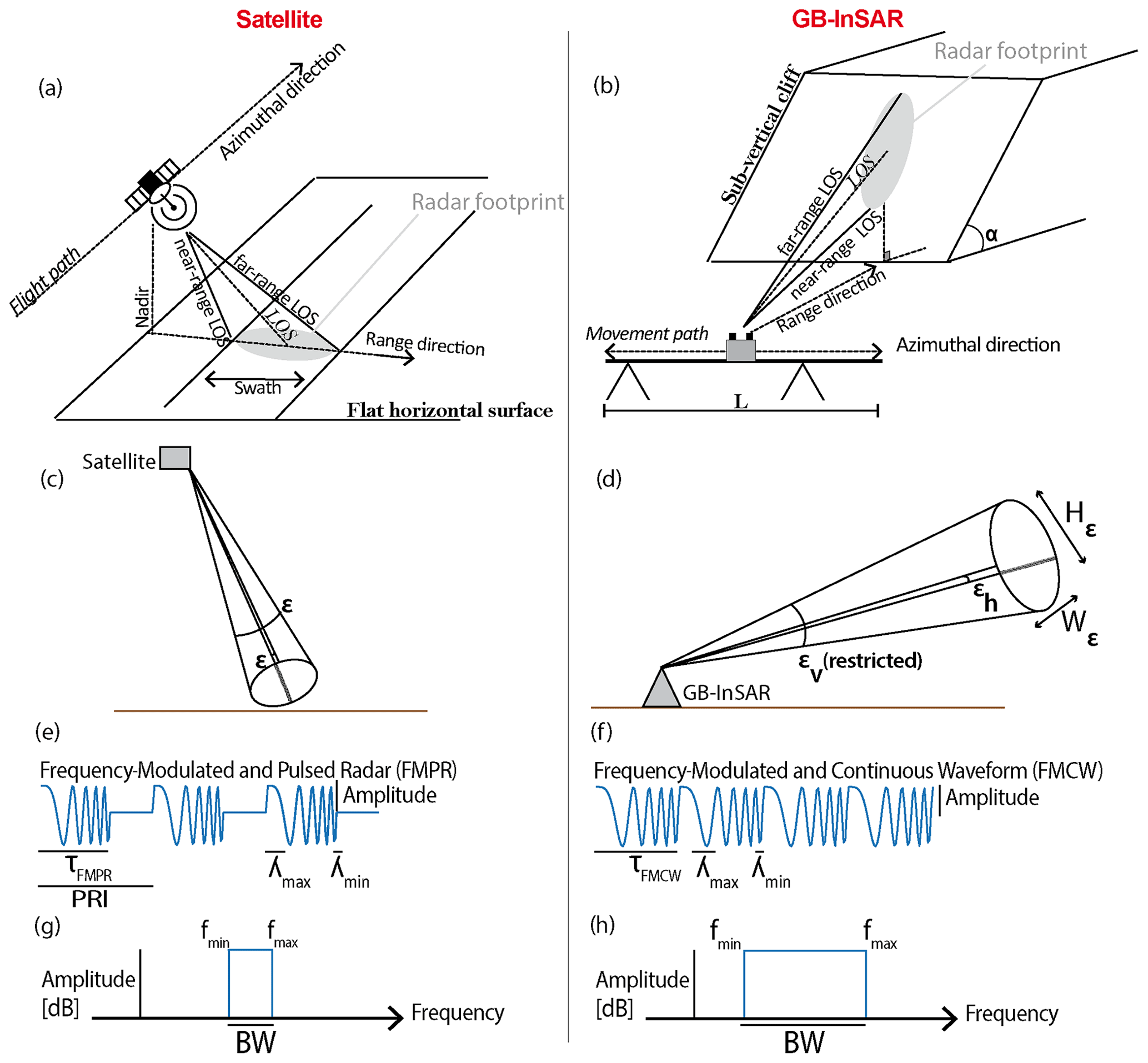
Figure 1 Illustration and comparison of radar acquisition characteristics in the case of satellite InSAR (a, c, e, g) and GB-InSAR (b, d, f, h). (a, b) Geometry of the acquisition defining the azimuthal and range directions. (c, d) Beamwidth characteristics. (e, f) Waveform characteristics. (g, h) Frequency characteristics.

In the case of the GB-InSAR, the azimuthal and range directions are parallel and perpendicular to the rail, respectively. The dLoS definition is similar to the aerial radar case, but the near-range is the line forming the smaller angle with the horizontal line, and the far-range is the larger angle (Fig. 1b).

2.1.2 Look angle or off-nadir angle Φ, incident angle θ, and depression angle γ

Look angle or off-nadir angle Φ, incident angle θ, and depression angle γ are well defined in the case of satellite imagery when the monitored surface is assumed to be sub-horizontal. The look angle Φ is the angle between the vertical line and the LoS. The depression angle γ is the complementary angle of the look angle. The definition of the incident angle θ is the same as in optical geometry, i.e. the angle between the LoS and the normal to the monitored surface (Fig. 2a and b). To simplify, when the monitored surface is horizontal for satellite InSAR or vertical for GB-InSAR, both θ and Φ are the angles between the LoS and the normal to the observed surface and are thus assumed to be equal.

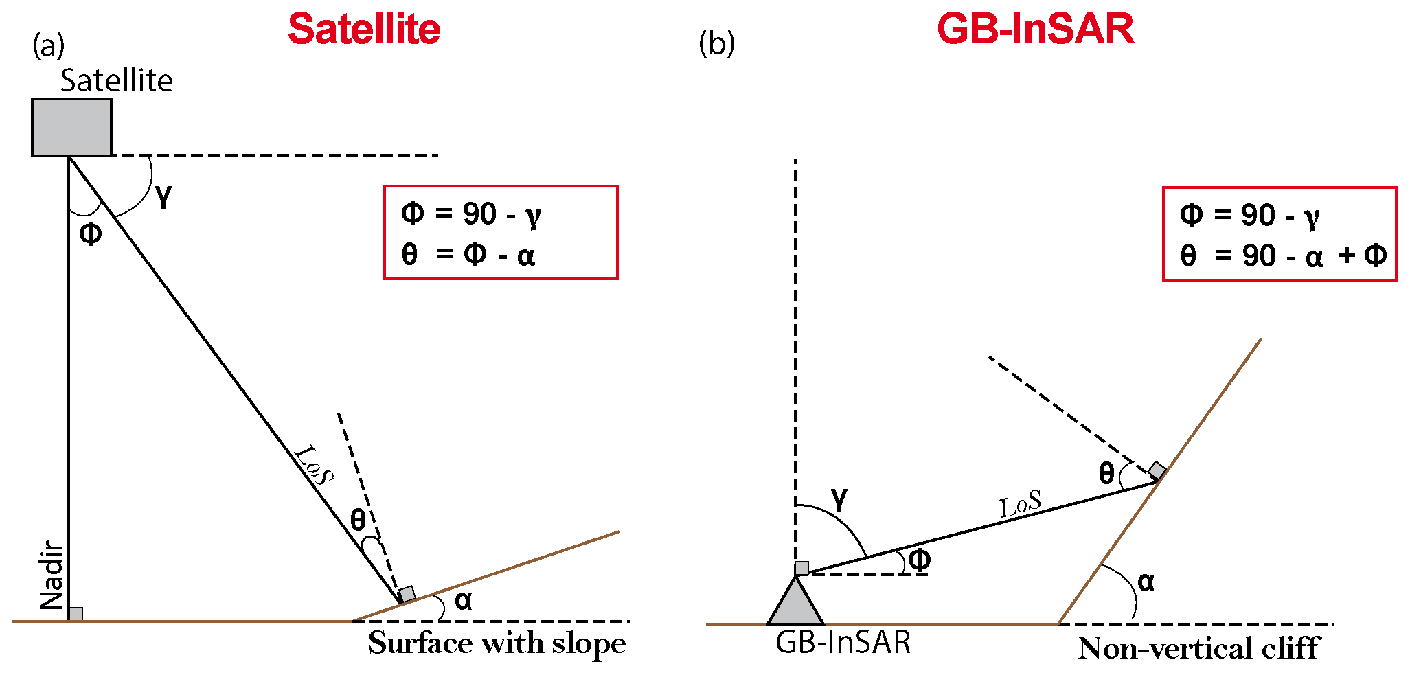
Figure 2 Illustration of the main specific angles used when describing a SAR acquisition. (a) Case of satellite radar acquisition. (b) Case of GB-InSAR acquisition.

2.1.3 Antenna beamwidth ε

The emitted signal propagates within a certain emission cone defined by an angle called beamwidth ε (Miron, 2006; Woodhouse, 2006), which is proportional to the wavelength according to diffraction laws (Lipson et al., 1995) and defines the maximum extent of the illuminated area. The radar footprint on the ground is an ellipsoid (Fig. 1a and b). Radar manufacturers provide antenna emission characteristics that are displayed in the form of a polar diagram (Toomay and Hannen, 2004). In the case of GB-InSAR, the vertical beamwidth ε_v is limited to 30° to avoid interferences with other radar devices such as planes (Anon, 2017; ETSI EN 300 440 v2.1.1), while the horizontal beamwidth ε_v is not legislatively restricted (Fig. 1d).

2.1.4 Radar bandwidth BW, satellite radar pulse length τ_FMPR, and GB-InSAR sweep length τ_FMCW

One of the major differences between GB-InSAR and satellite InSAR is related to their emitted signal. In the case of satellite InSAR, the transmitted signal must have sufficient amplitude to reach the Earth's surface and be backscattered with enough intensity to be detected by the radar receiver (Ferretti et al., 2014). However, the antennas are not able to continuously generate and send such a high-peak power signal. To overcome this technical limitation, the satellite radar signal is sent by pulses defined by a certain pulse duration τ_FMPR comprising between 10 and 100 µs, depending on the satellite (Fig. 1d). The emitted signal frequency is modulated to perform a pulse compression or chirping (Hein, 2004; Klauder et al., 1960). Such a radar can be named frequency-modulated pulsed radar (FMPR). The satellite radar bandwidth (BW; Fig. 1g) is the difference between the maximal and minimal emitted frequency. The time between two consecutive pulses is called the pulse repetition interval (PRI), and the duration of the emission of one pulse is the pulse length τ_FMPR.

The European Telecommunications Standards Institute (ETSI) defined some standards regarding the short-range devices (SRDs) emitting radio signals (Anon, 2017). The power and the frequencies of signals sent by terrestrial radar are limited to not interfere with other devices emitting and receiving radio signals. Specifically, for GB-InSAR operating in the frequency range of 17.1 to 17.3 GHz, the maximum limits for the frequency bandwidth and the power output are 200 MHz and 26 dBm, respectively.

GB-InSAR is considered a frequency-modulated continuous wave radar (FMCW radar; Wolff, 1998; Nadav, 2003), the signal emitted is of a lower intensity compared to satellite radar emissions. Since the signal is continuously emitted, one is lacking the timing necessary to isolate the backscattered signals and discriminate the range. This is achieved instead by modulating the frequency sent by the transmitter (Fig. 1f). The GB-InSAR bandwidth (BW; Fig. 1h) is the difference between the upper and lower cut-off frequencies. The duration of one sequence of frequency variation is the sweep length τ_FMCW.

BW, in the case of satellites, is generally smaller than for GB-InSAR, ranging between 10 and 80 MHz and between 70 and 200 MHz, respectively.

2.1.5 Real antenna length L_real and synthetic antenna length L

The azimuthal resolution is inversely proportional to the real antenna length L_real for RAR acquisition. In the case of SAR acquisition, a synthetic aperture antenna L is used to increase this resolution. For a GB-InSAR installed on a rail, the antenna length L corresponds to the rail length used to focus the radar image, which is in practice slightly shorter than the total rail length.

2.2 Spatial resolution

2.2.1 Radar and optical images

When representing the world (Fig. 3a and d) in an image, one must distinguish the radar image from the optical image, which is the visual display we are commonly used to seeing (Fig. 3b). The radar image is based on the distance between the radar antenna and each feature of the scene; the bottom line of the image corresponds to the monitored surface closest to the radar. Additionally, in radar geometry, range and azimuthal resolutions are defined differently, and by default, pixels are not square (Fig. 3c and e).

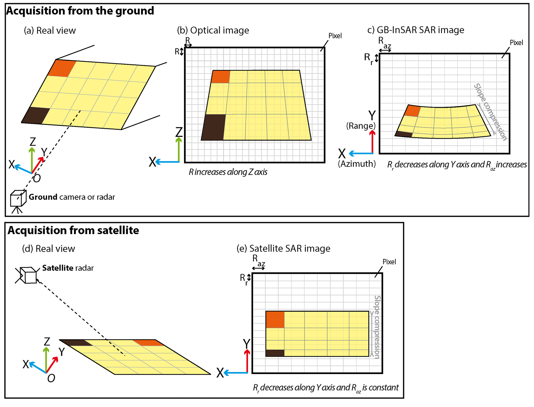
Figure 3 Comparison of the view of a surface area. (a) Real view in a parallel projection with the camera or radar acquiring the image from the ground. (b) Optical image taken with a camera from the ground. R increases with Z. Consequently, the distance between two consecutive horizontal lines decreases along Z. (c) GB-InSAR SAR image (after Tapete et al., 2013). R_az increases, and R_r decreases along Y. Consequently, the distance between two consecutive horizontal lines increases along Z. (d) Real view in a parallel projection with the satellite radar acquiring the image from the satellite orbit. (e) Satellite SAR image. R_az is constant along Y, while R_r decreases. Consequently, the distance between two consecutive horizontal lines increases along Y. In the case of the radar images (c, e), the slope is compressed compared to the optical image due to the foreshortening effect.

2.2.2 Azimuthal resolution R_az

The azimuthal resolution R_az corresponds to the resolution parallel to the flying trajectory in the case of satellite InSAR or parallel to the rail in the case of a linear GB-InSAR or to the horizontal resolution in the radar image. Its value differs between satellite InSAR and GB-InSAR.

The synthetic antenna aperture length being constrained by the rail length for the GB-InSAR, R_az, is related to the radar beamwidth (itself related to the wavelength λ), the range distance dLoS, and the synthetic antenna length L with the following relation (Henderson and Lewis, 1998; Jensen, 2006):

$$\begin{array}{}\text{(1)}& R_{\mathrm{az},\mathrm{GB}-\mathrm{InSAR}}={\displaystyle \frac{\mathrm{dLoS}\mathit{\lambda }}{\mathrm{2}L}}.\end{array}$$

Thus, R_az increases from the near- to far-range and the GB-InSAR image of a slope is a cone (Fig. 3d). Conversely, for the satellite, the synthetic aperture length L can be infinite, and R_az is dLoS-free and λ-free (Henderson and Lewis, 1998) and defined as follows:

$$\begin{array}{}\text{(2)}& R_{\mathrm{az},\mathrm{satellite}}={\displaystyle \frac{L_{\mathrm{real}}}{\mathrm{2}}}.\end{array}$$

The satellite InSAR image of a slope is thus rectangular (Fig. 3c).

Figure 4 presents the influence of dLoS and L on the azimuthal resolution in the case of the GB-InSAR.

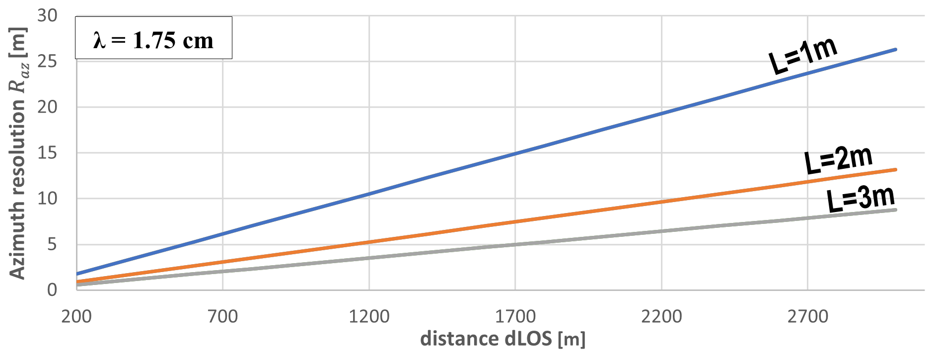
Figure 4 Influence of the rail length used to focus the GB-InSAR image corresponding to the synthetic antenna length L and the distance dLoS on the azimuthal resolution R_az for a Ku band with a wavelength equal to λ=1.75 cm. The longer the rail length, the better the azimuthal resolution will be.

2.2.3 Ground range resolution R_r

The ground range resolution R_r is the resolution along the LoS direction or the vertical resolution. It corresponds to the minimum time needed to distinguish two consecutive pulses (Woodhouse, 2006). It is ground-geometry-dependent and linked to the incidence angle θ, the speed of light c, and the pulse length τ_FMPR (after pulse compression) or sweep length τ_FMCW, according to the following relations (Henderson and Lewis, 1998; Jensen, 2006; Mahafza, 2000; McCandless and Jackson, 2004):

$$\begin{array}{}\text{(3)}& R_{\mathrm{r},\mathrm{satellite}}={\displaystyle \frac{{\mathit{\tau }}_{\mathrm{FMPR}}c}{\mathrm{2}\sin \mathit{\theta }}}={\displaystyle \frac{c}{\mathrm{2}\mathrm{BW}\sin \mathit{\theta }}}={\displaystyle \frac{c}{\mathrm{2}\mathrm{BW}\sin \left(\mathrm{\Phi }-{\mathit{\alpha }}_{\mathrm{app}}\right)}}.\end{array}$$

$$\begin{array}{}\text{(4)}& \begin{array}{rl}{R}_{\mathrm{r},\mathrm{GB}\text{-}\mathrm{InSAR}}& ={\displaystyle \frac{{\mathit{\tau }}_{\mathrm{FMCW}}c}{\mathrm{2}\sin \mathit{\theta }}}={\displaystyle \frac{c}{\mathrm{2}\mathrm{BW}\sin \mathit{\theta }}}\\ & ={\displaystyle \frac{c}{\mathrm{2}\mathrm{BW}\sin \left(\mathrm{90}-{\mathit{\alpha }}_{\mathrm{app}}+\mathrm{\Phi }\right)}}\\ & ={\displaystyle \frac{c}{\mathrm{2}\mathrm{BW}\cos \left(\mathrm{\Phi }-{\mathit{\alpha }}_{\mathrm{app}}\right)}}.\end{array}\end{array}$$

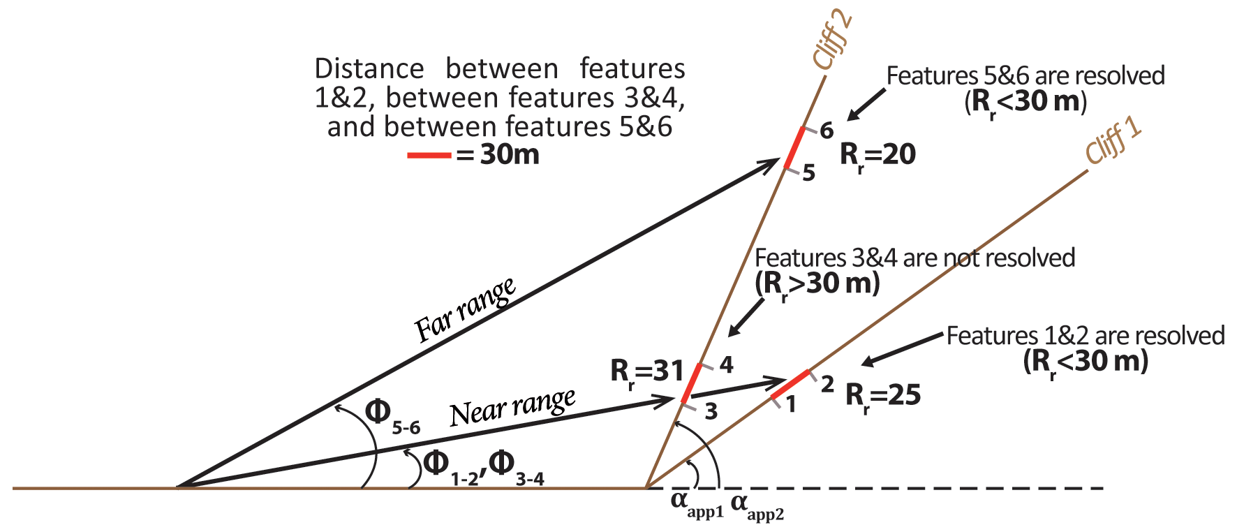
Figure 5 Ground range resolution R_r for two different slope angles and two different depression angles (adapted from Sabins, 1997). The distance between features 1 and 2, features 3 and 4, and features 5 and 6 is the same at 30 cm. However, features 1 and 2, located on a gentle slope and at a near-range distance from the GB-InSAR, are resolved (R_r=25 m); features 5 and 6 are located at a far-range distance on a steep slope and are also resoled (R_r=20 m), while features 3 and 4 are located on the same steep slope as features 5 and 6 but at a near-range distance and are not resolved (R_r=31 m).

The monitored cliff geometry has an impact on the range resolution with two major consequences, according to Eq. (4): (1) near-range surfaces and features possess, along a planar topography, less resolution in range than those in the far-range because Φ increases with the range, and (2) steeper slopes increase the range resolution by increasing α_app (Fig. 5; Sabins, 1997; Stimson, 1998; Jensen, 2006). Furthermore, the shorter the pulse length τ_FMPR or sweep length τ_FMCW, the finer the resolution will be. Nevertheless, one must be careful with the choice of the pulse length because if a short τ_FMPR or τ_FMCW results in a better resolution, then the backscatter signal is also weaker and might not be detected if too low. For GB-InSAR, the parameter that can be chosen by the user is the bandwidth (BW). The further away the radar is installed from the target area, the smaller the bandwidth should be to be sure to detect the backscattered signal. A good balance between an acceptable resolution and a sufficiently strong backscattered signal must be found (Fig. 6a and b).

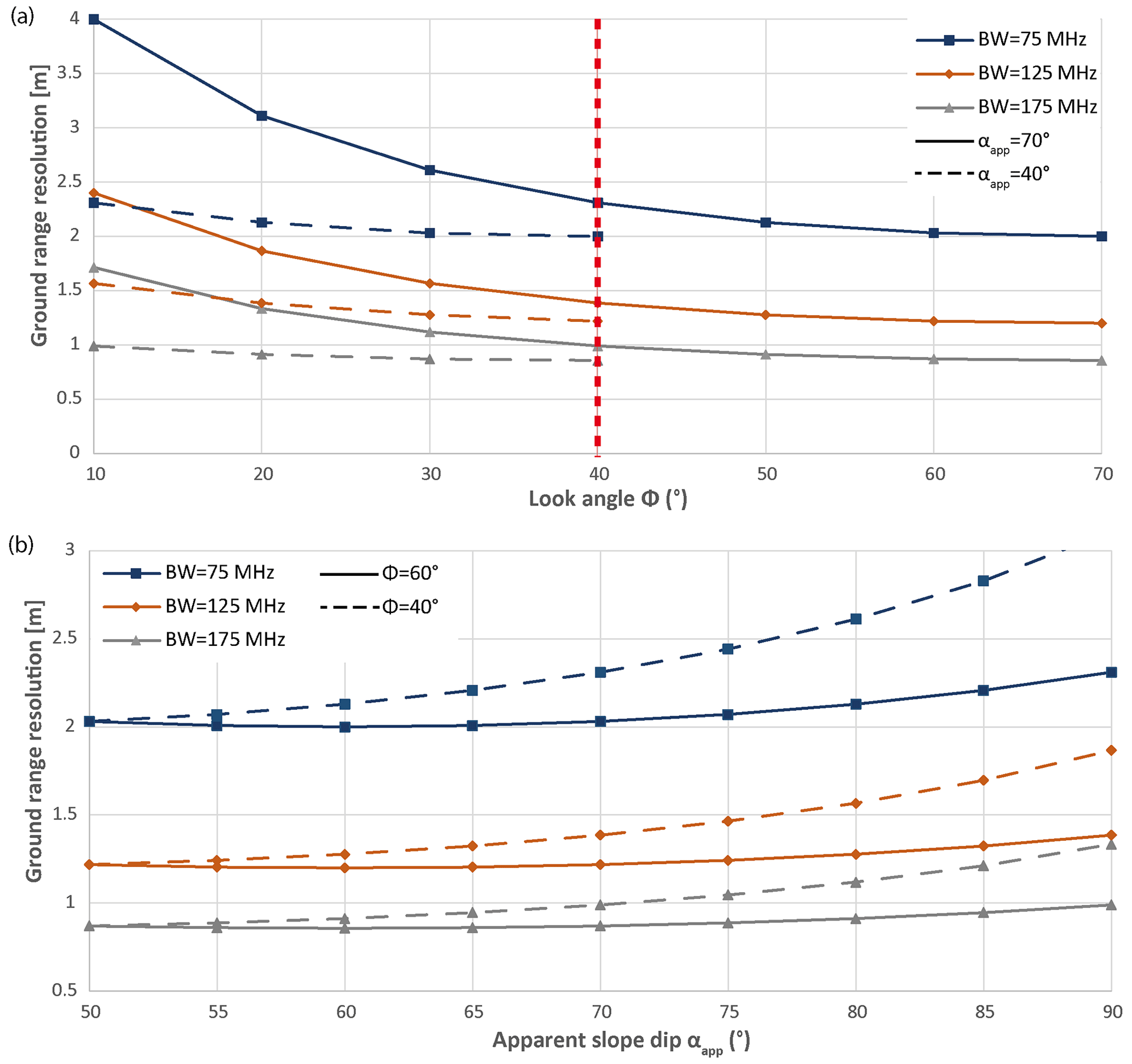
Figure 6 Influence of some GB-InSAR parameters on the range resolution R_r. (a) Influence of the look angle Φ for different BWs. It is interesting to notice that the resolution varies a little when Φ is larger than 40°. (b) Influence of the apparent slope dip α_app for different BWs.

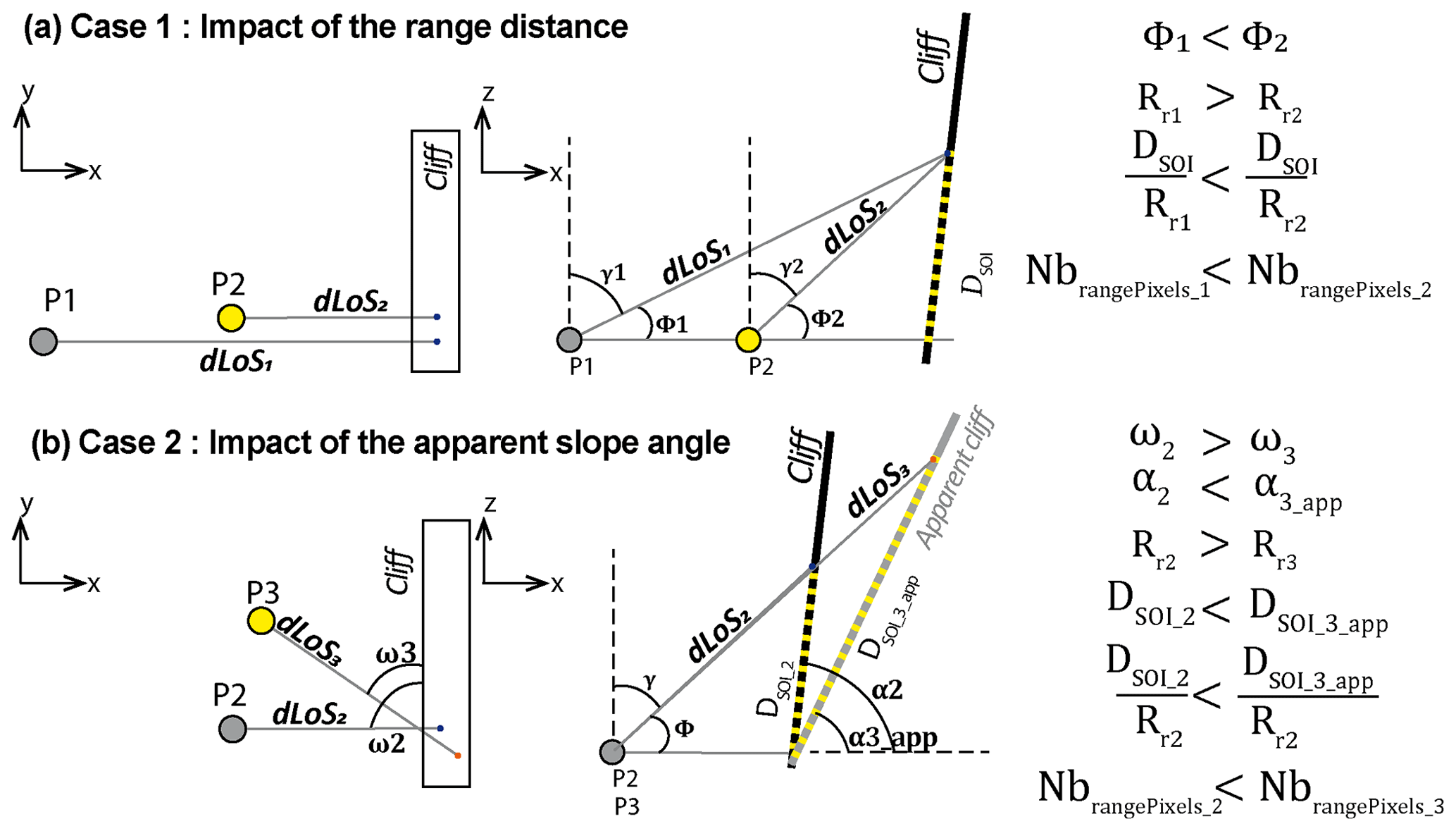
Figure 7 Two scenarios of the selection of the best GB-InSAR installation to get the lower compression of the SoI in range. The best location is highlighted in yellow. (a) Case 1 shows the installation near vs. far from the monitored cliff. (b) Case 2 shows the installation in front of vs. aside the monitored cliff. When looking from the aside position, α_app is smaller according to Eq. (6), and the apparent SoI length on slope in the radar direction is longer so the information is distributed across more pixels within the range distance.

2.2.4 Number of pixels and slope compression

During a monitoring campaign, the surveyor focuses on a slope of interest (SoI). A monitoring campaign is effective when information concerning this SoI is distributed across a wide range of pixels rather than compressed within a few; this involves attempting to get the finest possible range resolution. The position of the GB-InSAR will have an influence on the resolution, and the number of pixels in which the SoI will be contained can be estimated with the following formula:

$$\begin{array}{}\text{(5)}& {\mathrm{Nb}}_{\mathrm{pixelRange}}={\displaystyle \frac{D_{\mathrm{SoI}}}{R_{\mathrm{r}}}},\end{array}$$

where D_SoI is the distance along the monitored slope of the SoI.

The steeper the slope, the more the information will be compressed, and some interesting features may be contained in the same pixel. Given this consideration, if one has the choice between two radar installations, it is worth (1) reducing the range distance (Fig. 7a) and (2) reducing the apparent slope angle α_app of the measured cliff to increase the apparent SoI distance (Fig. 7b). The apparent slope angle can be reduced by placing the radar aside instead of in front of the measured slope and by applying the following equations (Addie, 1968):

$$\begin{array}{}\text{(6)}& {\displaystyle }& {\displaystyle }{\mathit{\alpha }}_{\mathrm{app}}={\tan }^{-\mathrm{1}}(\tan \mathit{\alpha }\times \sin \mathit{\omega }),\text{(7)}& {\displaystyle }& {\displaystyle }\mathit{\omega }={\mathit{\omega }}_{\mathrm{LoS}}-{\mathit{\omega }}_{\mathrm{slope}},\end{array}$$

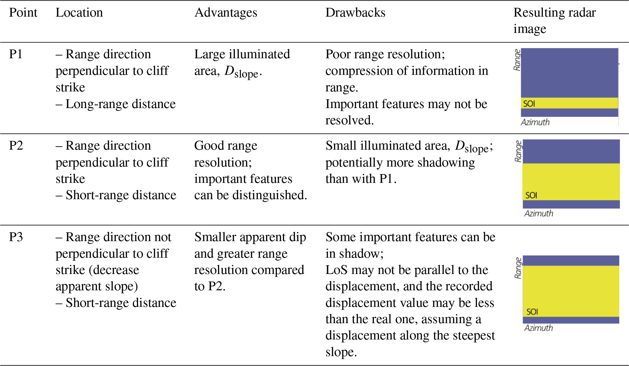
with ω being the angle between the slope direction and the LoS direction, and ω_LoS and ω_slope being the orientation of the LoS toward north and the slope strike, respectively. Table 2 lists the advantages and drawbacks of each radar position.

Table 2 Advantages and drawbacks of each radar position presented in Fig. 7.

2.3 Shadow, foreshortening, and layover

The following three geometrical notions must be restated about radar geometry because they can trigger noise and/or loss of information (Jensen, 2006):

• Foreshortening. Any terrain with a slope α inclined toward the radar (fore slope) results in a compression and a brightening of its surface in the radar image, also called foreshortening. Conversely, slopes inclined away from the radar (back slope) appear darker and elongated in the image (Fig. 8a). The foreshortening factor F_f can be defined as follows:

  $$\begin{array}{}\text{(8)}& F_{\mathrm{f}}=\sin (\mathit{\alpha }-\mathrm{\Phi }).\end{array}$$

• Layover. If the fore slope angle is greater than the look angle Φ, then one can observe layover. The backscatter signal of the layover object will reach the radar receiver before the backscatter signal of the object located before. The information contained in the signal will be stored in the previous pixel in the range of the image, resulting in a layover distortion of the image which cannot be corrected. With a GB-InSAR, layover effects occur in the case of an overhanging wall (Fig. 8b).

• Shadow. An area hidden by a slope or by any other feature is not illuminated by the radar and will not be seen in the radar image, resulting in a loss of information. This can be, for instance, a deep valley or the ground behind a tall building (Fig. 8c).

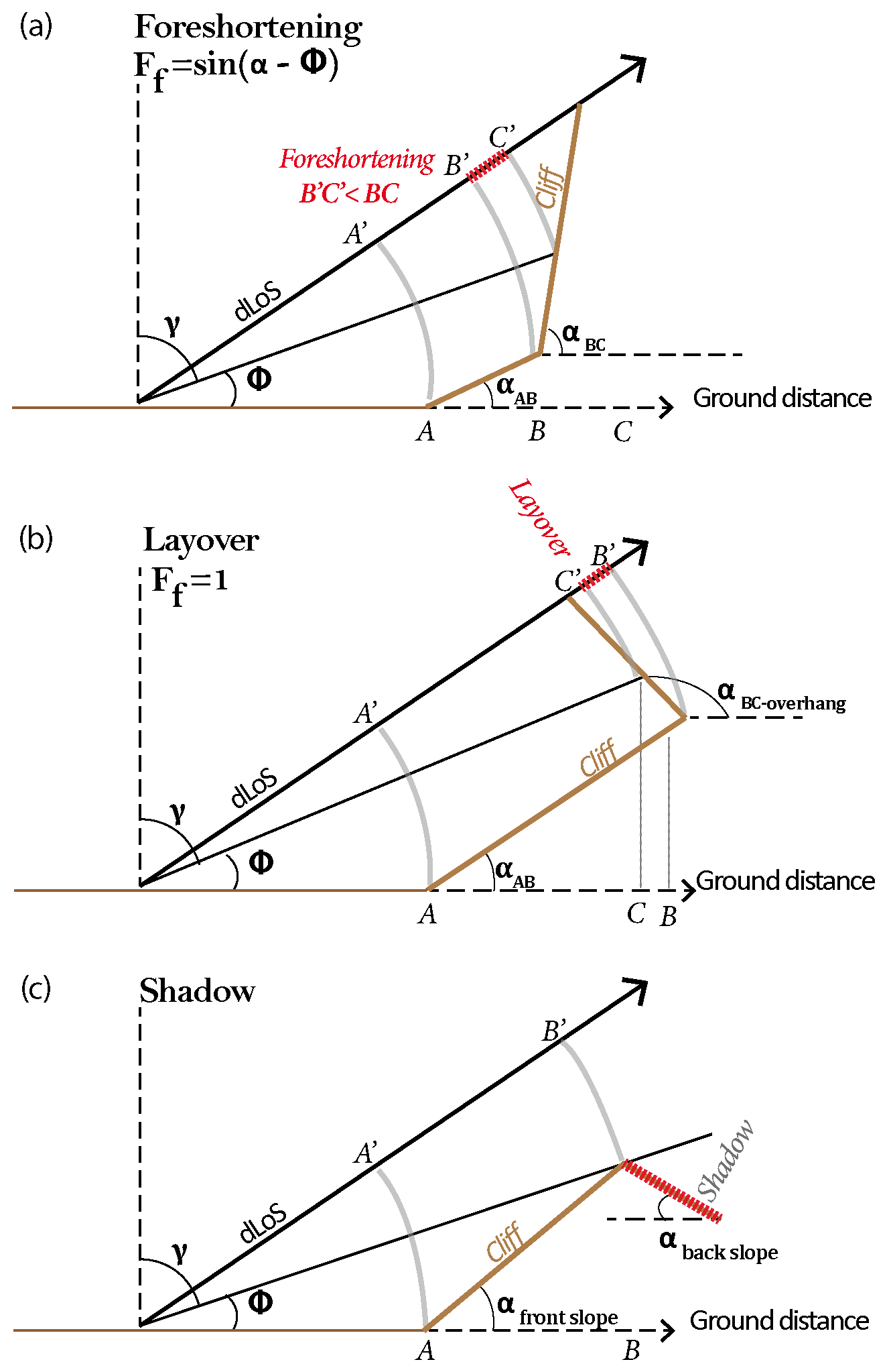
Figure 8 Illustration of geometrical artefacts in the case of GB-InSAR. (a) Foreshortening. (b) Layover. (c) Shadow effects.

3 Methodology

3.1 GB-InSAR constrains

In a review, Caduff et al. (2015) present a list of points to carefully consider when choosing the location for the GB-InSAR installation, including the visibility of the target area, the SoI, the foreshortening effects, the expected displacement (rate, direction, and mechanism), the atmospheric influences, and the technical constraints (hardware, setup, accessibility, etc.).

The MATLAB tool presented here is aimed at estimating some of those parameters and choosing the best location when several options are possible. The constraints estimated with the tool are the following:

• The range distance dLoS; the bandwidth (BW) must be adjusted based on this distance. In any case, the target should not be further than 4 or 5 km away, depending on the GB-InSAR device, to avoid the risk of a backscatter signal amplitude that is too weak.

• The resolution in range and in azimuth; once the potential location is found, it is worth estimating the resolution that will be obtained, as well as the extent of the surface illuminated by the radar.

• The areas in shadow and those subject to a strong foreshortening.

3.2 Input parameters

3.2.1 The DEM

The MATLAB tool requires as first input a digital elevation model (DEM) in ASCII format that is cropped around the area of interest. The MATLAB code converts it into a 3D point cloud which is displayed in a window. For the use that will be made of the DEM, a resolution of 5 m is sufficient. For each pixel of the grid, the dip and dip direction is calculated with the function “gradient” (MATLAB, 2023). Additionally, the user provides the coordinates of the centre of the area of interest and of the location where they consider installing the radar.

3.2.2 Radar parameters

The parameters that will be estimated are related to the radar characteristics described above (L, BW, and ε) and must be set up by the user before starting the computation because they influence the resulting resolution, as well as the extent of the illuminated area. Since the vertical beamwidth is limited in the case of the GB-InSAR, the vertical and horizontal beamwidths are, respectively, selected by the user and denoted ε_v and ε_h.

3.3 Estimation of output radar results

3.3.1 Fore slope and distance maps

First, when installing the radar, the distance between the radar and the target surface must be estimated to not be greater than 4 or 5 km. Once the location of the radar (x_radar, y_radar, and z_radar) is provided, a map is displayed that gives for each point of coordinates (x_target, y_target, and z_target) the distance to the radar, which is defined by

$$\begin{array}{}\text{(9)}& \mathrm{distance}=\sqrt{\mathrm{\Delta }{x}^{\mathrm{2}}+\mathrm{\Delta }{y}^{\mathrm{2}}+\mathrm{\Delta }{z}^{\mathrm{2}}},\end{array}$$

with $\mathrm{\Delta }x=x_{\mathrm{target}}-x_{\mathrm{radar}}$, $\mathrm{\Delta }y=y_{\mathrm{target}}-y_{\mathrm{radar}}$, and $\mathrm{\Delta }z=z_{\mathrm{target}}-z_{\mathrm{radar}}$. Slopes facing the radar – or fore slope – can result in foreshortening effect, whereas slopes facing away – or back slope – will always be in the shadow. That information is displayed in a second map, where the fore slope points have a value of 1, and the other points have a value of −1. To produce this map, the apparent dip α_app is computed for each point with Eq. (6). The fore- and back slopes are deduced from α_app as follows:

$$\begin{array}{}\text{(10)}& {\displaystyle }& {\displaystyle }\mathrm{If}{\mathit{\alpha }}_{\mathrm{app}}>\mathrm{0}\to \mathrm{fore}\mathrm{slope}.\text{(11)}& {\displaystyle }& {\displaystyle }\mathrm{If}{\mathit{\alpha }}_{\mathrm{app}}<\mathrm{0}\to \mathrm{back}\mathrm{slope}.\end{array}$$

3.3.2 Radar footprint and illuminated area estimation

The radar footprint is an ellipse within which the user selects a smaller area to focus the radar acquisition. This illuminated surface is selected by choosing the minimum and maximum azimuth Az°_min and Az°_max and the minimum and maximum range R_min and R_max of the acquisition and should encompass the whole instable area to be monitored, as well as a supposedly stable area, in order to determine the necessary atmospheric corrections (Noferini et al., 2005; Pipia et al., 2008) and the post-processing unwrapping (Goldstein et al., 1988).

Before installing the radar and starting the acquisition, it is worth checking the maximum possible radar footprint, as well as the illuminated surface, according to the batch of azimuths and ranges selected by the user.

Once the radar and the target location are selected, the map is updated to display the footprint and the points illuminated by the radar during the acquisition according to the parameters R_min, R_max, Az°_min, and Az°_max selected by the user.

To do so, the coordinates of each point of the point cloud are converted from the global geographical coordinate system “global” in a local coordinate system “local”, whose frame origin is the centre of the region of interest selected by the user. The X axis is horizontal and perpendicular to the LoS direction, and the horizontal Y axis is perpendicular to X. The Z axis is a vertical unit vector. Thus, the unit vectors of the local frame are

$$\begin{array}{}\text{(12)}& \begin{array}{rl}& {\left(\begin{array}{c}{\mathit{X}}_{\mathrm{unit}}\\ {\mathit{Y}}_{\mathrm{unit}}\\ {\mathit{Z}}_{\mathrm{unit}}\end{array}\right)}_{\mathrm{local}}\\ & =\left(\begin{array}{llc}\frac{\mathrm{\Delta }{\mathit{y}}_{\mathrm{global}}}{\sqrt{\mathrm{\Delta }{\mathit{y}}_{\mathrm{global}}^{\mathrm{2}}+\mathrm{\Delta }{\mathit{x}}_{\mathrm{global}}^{\mathrm{2}}}}& \frac{\mathrm{\Delta }{\mathit{x}}_{\mathrm{global}}}{\sqrt{\mathrm{\Delta }{\mathit{y}}_{\mathrm{global}}^{\mathrm{2}}+\mathrm{\Delta }{\mathit{x}}_{\mathrm{global}}^{\mathrm{2}}}}& \mathrm{0}\\ \frac{\mathrm{\Delta }{\mathit{x}}_{\mathrm{global}}}{\sqrt{\mathrm{\Delta }{\mathit{y}}_{\mathrm{global}}^{\mathrm{2}}+\mathrm{\Delta }{\mathit{x}}_{\mathrm{global}}^{\mathrm{2}}}}& \frac{\mathrm{\Delta }{\mathit{y}}_{\mathrm{global}}}{\sqrt{\mathrm{\Delta }{\mathit{y}}_{\mathrm{global}}^{\mathrm{2}}+\mathrm{\Delta }{\mathit{x}}_{\mathrm{global}}^{\mathrm{2}}}}& \mathrm{0}\\ \mathrm{0}& \mathrm{0}& \mathrm{1}\end{array}\right).\end{array}\end{array}$$

Each point coordinate can be converted from the global geographical coordinate system to the new local coordinate system by applying a translation T defined by the vector $\mathit{L}\mathit{o}\mathit{S}\left(\begin{array}{c}\mathrm{\Delta }{\mathit{x}}_{\mathrm{global}}\\ \mathrm{\Delta }{\mathit{y}}_{\mathrm{global}}\\ \mathrm{\Delta }{\mathit{z}}_{\mathrm{global}}\end{array}\right)$, followed by a rotation of matrix Ω:

$$\begin{array}{}\text{(13)}& \left\{\begin{array}{l}T=\left(\begin{array}{c}\mathrm{\Delta }{\mathit{x}}_{\mathrm{global}}\\ \mathrm{\Delta }{\mathit{y}}_{\mathrm{global}}\\ \mathrm{\Delta }{\mathit{z}}_{\mathrm{global}}\end{array}\right)\\ \mathbf{\Omega }=\left(\begin{array}{lcl}\mathit{a}& -\mathit{b}& \mathbf{0}\\ \mathit{b}& \mathit{a}& \mathbf{0}\\ \mathbf{0}& \mathbf{0}& \mathbf{1}\end{array}\right)\end{array}\right..\end{array}$$

The relation linking the coordinates of each point in the global geographical coordinate system and the new local coordinate system is

$$\begin{array}{}\text{(14)}& {\displaystyle }{\left(\begin{array}{c}\mathit{x}\\ \mathit{y}\\ \mathit{z}\end{array}\right)}_{\mathrm{local}}=\mathbf{\Omega }\cdot {\left(\begin{array}{c}\mathit{x}\\ \mathit{y}\\ \mathit{z}\end{array}\right)}_{\mathrm{global}}+T\text{(15)}& {\displaystyle }\begin{array}{rl}{\left(\begin{array}{c}\mathit{x}\\ \mathit{y}\\ \mathit{z}\end{array}\right)}_{\mathrm{local}}& =\underset{\mathrm{rotation}\mathrm{matrix}}{\underbrace{\left(\begin{array}{clc}\mathit{a}& -\mathit{b}& \mathbf{0}\\ \mathit{a}& \mathit{b}& \mathbf{0}\\ \mathbf{0}& \mathbf{0}& \mathbf{1}\end{array}\right)}}\cdot {\left(\begin{array}{c}\mathit{x}\\ \mathit{y}\\ \mathit{z}\end{array}\right)}_{\mathrm{global}}\\ & +\underset{\mathrm{translation}\mathrm{matrix}}{\underbrace{\left(\begin{array}{c}\mathrm{\Delta }{\mathit{x}}_{\mathrm{global}}\\ \mathrm{\Delta }{\mathit{y}}_{\mathrm{global}}\\ \mathrm{\Delta }{\mathit{z}}_{\mathrm{global}}\end{array}\right)}}.\end{array}\end{array}$$

The pair of values (a, b) is found by solving the system with the coordinates of the target point ${\left(\begin{array}{c}\mathrm{0}\\ \mathrm{0}\\ \mathrm{0}\end{array}\right)}_{\mathrm{local}}$ in the local coordinate system:

$$\begin{array}{}\text{(16)}& \begin{array}{rl}{\left(\begin{array}{c}\mathrm{0}\\ \mathrm{0}\\ \mathrm{0}\end{array}\right)}_{\mathrm{local}}& =\left(\begin{array}{clc}a& -b& \mathrm{0}\\ b& a& \mathrm{0}\\ \mathrm{0}& \mathrm{0}& \mathrm{1}\end{array}\right)\cdot {\left(\begin{array}{c}{x}_{\mathrm{target}}\\ y_{\mathrm{target}}\\ z_{\mathrm{target}}\end{array}\right)}_{\mathrm{global}}\\ & +\left(\begin{array}{c}\mathrm{\Delta }{x}_{\mathrm{global}}\\ \mathrm{\Delta }{y}_{\mathrm{global}}\\ \mathrm{\Delta }{z}_{\mathrm{global}}\end{array}\right)\end{array}\end{array}$$

All points of the point cloud are converted into the new local coordinate system with Eq. (13). It is then possible to filter points that belong to the radar footprint, knowing ε_v and ε_h (Fig. 9a). A point $P(x_{\mathrm{local}},y_{\mathrm{local}},z_{\mathrm{local}})$ is within the footprint if

$$\begin{array}{}\text{(17)}& \mathrm{|}{z}_{\mathrm{local}}\mathrm{|}<\sqrt{H_{\mathit{\epsilon }}^{\mathrm{2}}-{\left({\displaystyle \frac{x_{\mathrm{local}}}{L_{\mathit{\epsilon }}}}\right)}^{\mathrm{2}}},\end{array}$$

with

$$\begin{array}{}\text{(18)}& {\displaystyle }& {\displaystyle }{L}_{\mathit{\epsilon }}=\mathrm{dLoS}\left(O\right)\cdot \tan {\mathit{\epsilon }}_{\mathrm{h}}\text{(19)}& {\displaystyle }& {\displaystyle }{H}_{\mathit{\epsilon }}=\mathrm{dLoS}\left(O\right)\cdot \tan {\mathit{\epsilon }}_{\mathrm{v}}.\end{array}$$

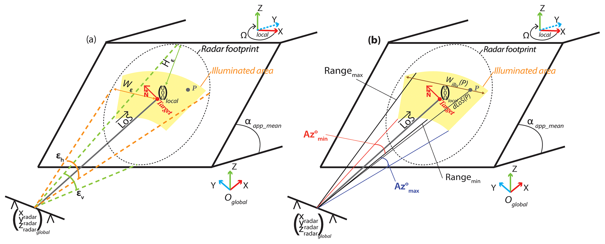
Figure 9 Illustration of the change in the coordinate frame from a global one $(X,Y,Z{)}_{\mathrm{global}}$ to a local one $(X,Y,Z{)}_{\mathrm{local}}$, centred on the target coordinates and aiming at highlighting the points of the point cloud within the radar footprint and the illuminated area. The X_local axis is horizontal and perpendicular to LoS, and the Y_local axis is horizontal and perpendicular to X_local. (a) Point P is within the radar footprint because its coordinates answer the conditions defined in Eq. (16). (b) Point P is illuminated because its coordinates answer the conditions defined in Eq. (19).

Points belonging to the illuminated area are extracted in a second step. A point $P(x_{\mathrm{local}},y_{\mathrm{local}},z_{\mathrm{local}})$ is within the illuminated area if (Fig. 9b)

$$\begin{array}{}\text{(20)}& \left\{\begin{array}{l}P\mathit{ϵ}\mathrm{footprint}\\ \mathrm{dLoS}\left(P\right)\mathit{ϵ}\left[R_{\min };R_{\max }\right]\\ z_{\mathrm{local}}\mathit{ϵ}\left[W_{\min }\left(P\right);W_{\max }\left(P\right)\right]\end{array}\right.,\end{array}$$

with

$$\begin{array}{}\text{(21)}& \left\{\begin{array}{l}{W}_{{\mathrm{illu}}_{\min }}\left(P\right)=\mathrm{dLoS}\left(P\right)\cdot \tan \mathrm{Az}{\mathit{°}}_{\min }\\ W_{{\mathrm{illu}}_{\max }}\left(P\right)=\mathrm{dLoS}\left(P\right)\cdot \tan \mathrm{Az}{\mathit{°}}_{\max }\end{array}\right..\end{array}$$

Once the points illuminated by the radar are known, a mean square method (Wolberg, 2006) is used to determine the mean plan intersecting the illuminated points defined by its normal vector N. This vector is then converted into the mean slope dip α_MEAN and the mean slope dip direction ω_MEAN.

3.3.3 Resolution, foreshortening, and layover maps

Equations (1) and (4) are applied on each point of the point cloud to estimate the range and azimuthal resolutions, and the result is displayed in two distinct maps.

With the mean plan dip direction ω_MEAN and dip α_MEAN being known, the latter is converted in apparent dip from the radar position α_{MEAN_app}, and the foreshortening for this mean plan F_f-MEAN is calculated by applying Eq. (8), giving a value comprised between [0; 1], with 0 for no foreshortening and 1 for the beginning of layover. In addition, the foreshortening degree is calculated for each point of the point cloud.

It is then possible to estimate for each point if it will be affected by a stronger or a weaker foreshortening than the mean slope plan by subtracting the mean plan foreshortening F_f-MEAN from the foreshortening calculated at each point. Such a map is also one of the outputs of the tool. A negative or positive value implies, respectively, a weaker or stronger foreshortening at that point than the mean one.

3.4 Tool interface

The application coded in MATLAB is presented in a graphical user interface (Fig. 10). The users first select the DEM to import and convert into a 3D point cloud. They then give the coordinates of the location where they consider installing the radar, as well as the coordinates corresponding to the center (or middle) of the region of interest. It can be found directly on the point cloud or from a GPS measurement performed on the field. The radar parameters, listed in Table 3, must also be given before starting the computation. To filter pixels within the area illuminated during the processing, the user also gives the minimum and maximum ranges and azimuths.

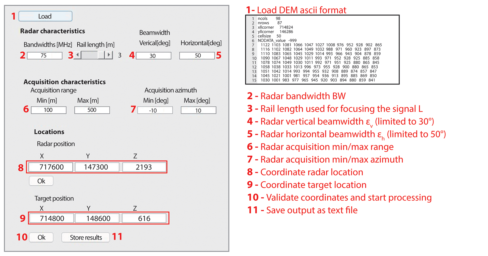
Figure 10 Interface of the MATLAB tool and the format of the DEM grid to import in a text file format.

Table 3 Characteristics of the LiSA GB-InSAR used in this study.

At the end of the processing, the different maps are displayed in 3D and can be saved as a text file to be reused later.

4 Description of the tested case studies

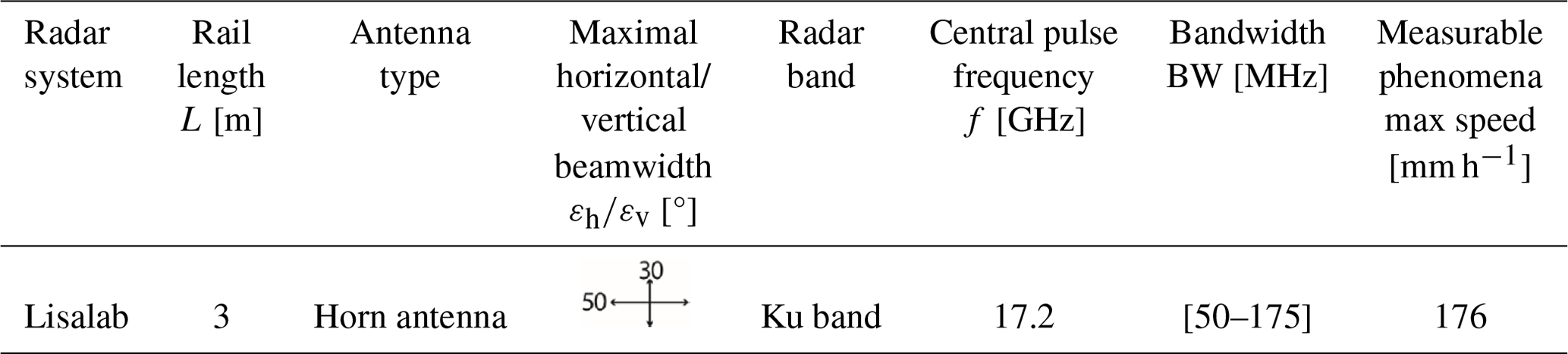
To validate the results obtained with this tool, the latter has been tested with a Lisalab GB-InSAR (Table 3) on (1) a simple synthetic cliff created in CloudCompare, facing north and with a progressive slope and a back slope (Fig. 11), and (2) two real cliffs where GB-InSAR monitoring campaigns were conducted (Table 4; Figs. 12 and 13).

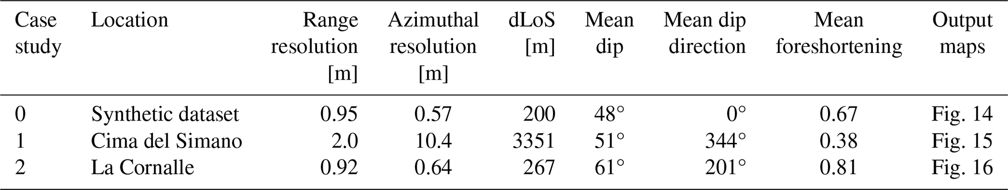
Table 4 The three study cases with their DEM characteristics and the radar parameters chosen.

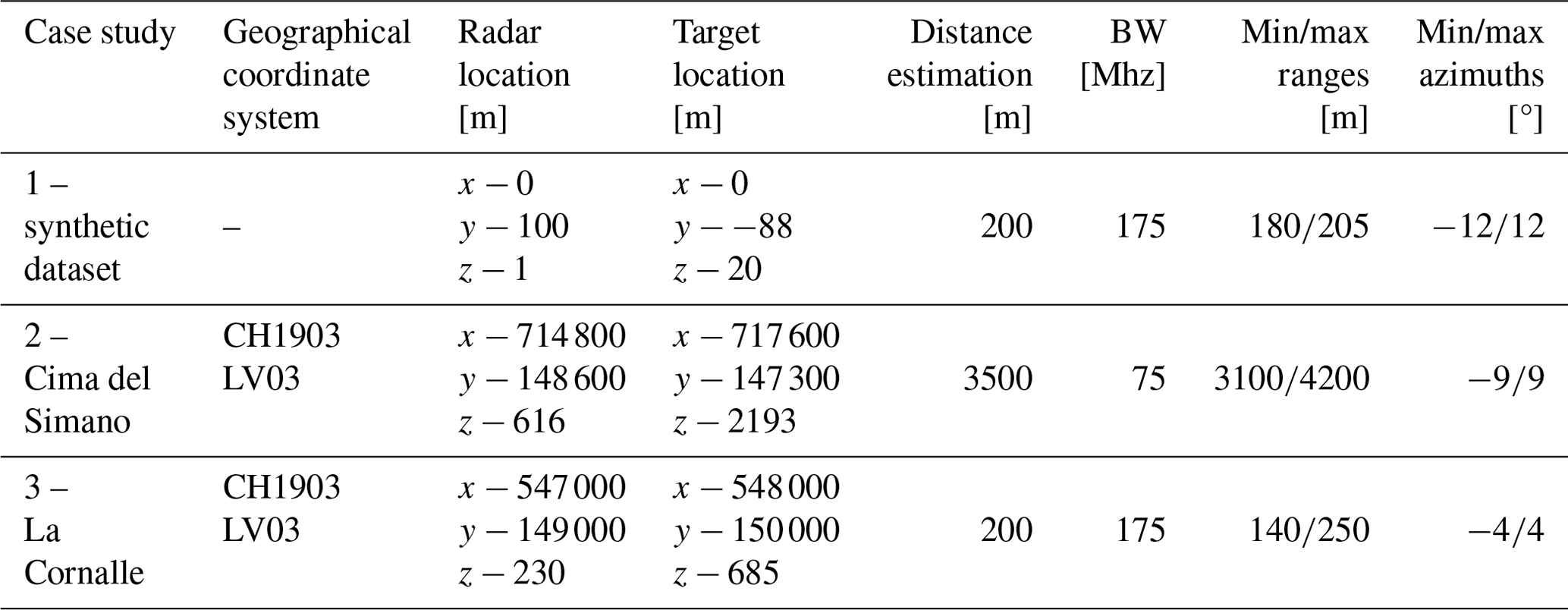
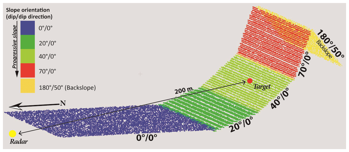
Figure 11 Synthetic dataset of a cliff facing north with a progressive slope dip and a back slope.

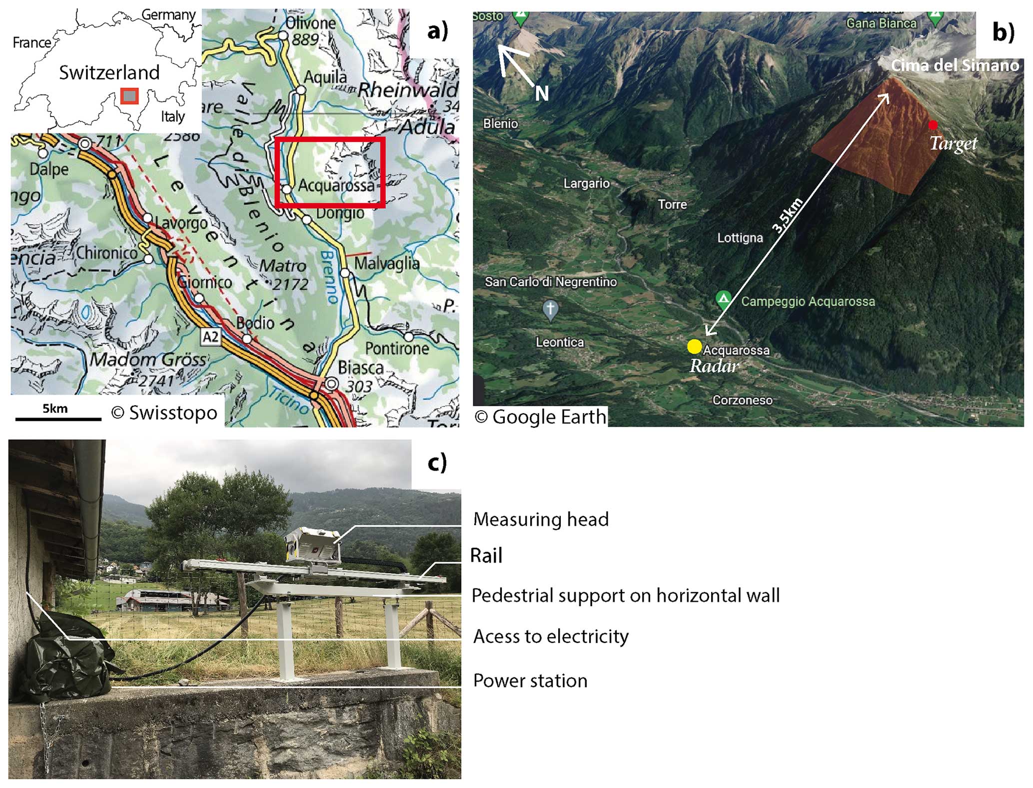
Figure 12 First real studied site at Cima del Simano. (a) Location. (b) Radar and target location shown in the Google Earth © 2022 image. (c) Lisalab GB-InSAR installation.

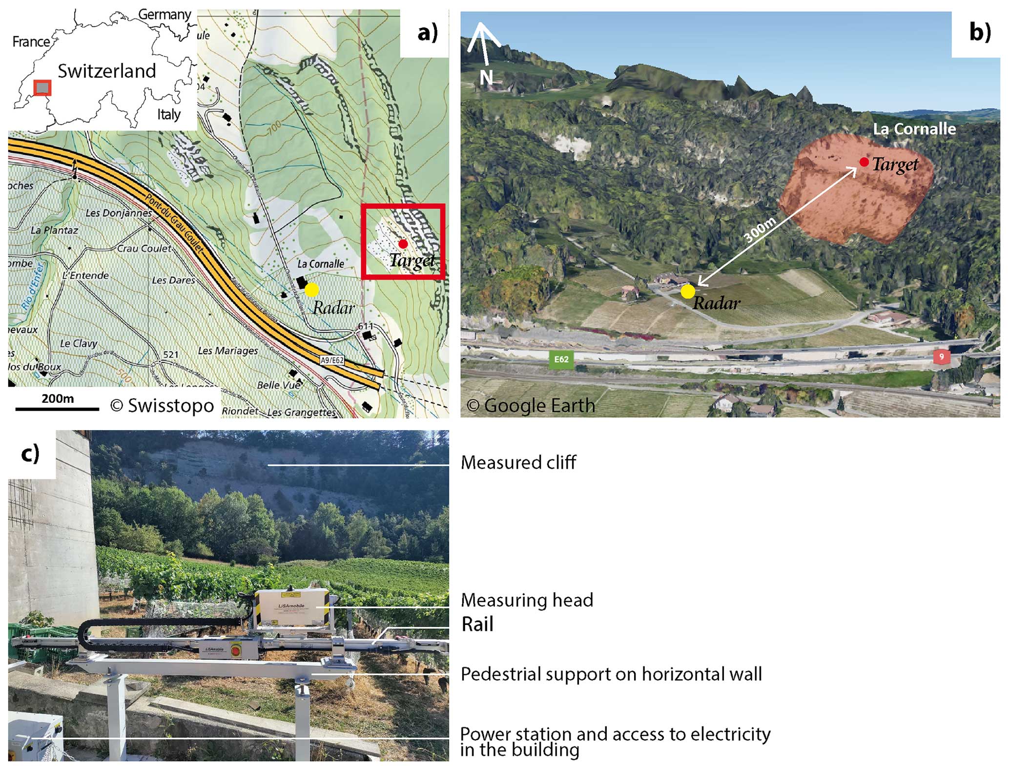
Figure 13 Second real studied site at La Cornalle cliff. (a) Location. (b) Radar and target location shown in the Google Earth © 2022 image. (c) Lisalab GB-InSAR installation.

4.1 Real case 1: Cima del Simano instability monitoring

Cima del Simano is a deep-seated landslide located in the Ticino canton in Switzerland (Fig. 12a). Satellite interferometry measurements highlight the presence of slow sub-vertical gravitational movements on top of the mountain which motivated the launch of a GB-InSAR monitoring campaign in 2021 (Wolff et al., 2023). A Lisalab GB-InSAR with a 3 m rail was installed in the valley near a building belonging to the Acquarossa commune in order to have access to an electrical power supply (Fig. 12c). The acquisition is challenging because the radar is located at its range limit, and the top of the cliff, at an altitude of 2500 m, witnesses strong atmospheric effects (Fig. 12b).

4.2 Real case 2: La Cornalle cliff monitoring

La Cornalle cliff, located in the Lavaux vineyard (east Lausanne, Switzerland; Fig. 13a), has been monitored with yearly lidar acquisitions since 2013 (Carrea et al., 2014, 2015). This steep cliff is affected by erosion processes, and frequent rockfall events occur every year (Fig. 13b). This site is monitored to estimate the role of the rock surface temperature and of the atmospheric erosion (Fei et al., 2023). For this purpose, a GB-InSAR has been installed in August 2022 at the bottom of the cliff. The Lisalab rail has been set up on a flat wall near a factory in the vineyard to have access to electricity and also very near the cliff to get the best possible resolution (Fig. 13c).

5 Results

The obtained results are summarized in Table 5 for the three studied cases, and some output maps are displayed in Fig. 14 in the case of the synthetic dataset, in Fig. 15 in the case of Cima del Simano, and in Fig. 16 for La Cornalle cliff. The extra output maps are available in Figs. A1–A3.

Table 5 Results obtained with the MATLAB tool for the three study sites.

5.1 Synthetic dataset (Figs. 14 and A1)

With a LoS distance of 200 m, the range and azimuthal resolutions are, respectively, 0.95 and 0.57 m at the target location. The calculated apparent mean dip is 48° because the illuminated area encompasses a major part of the slope with a dip of 40° and a little part of the slope with a dip of 70°. The mean foreshortening of the SoI is 0.67 (Fig. 14e), but the points located on the slope with a dip of 40° are less affected by foreshortening than those located on the slope with a dip of 70° (Fig. 14f).

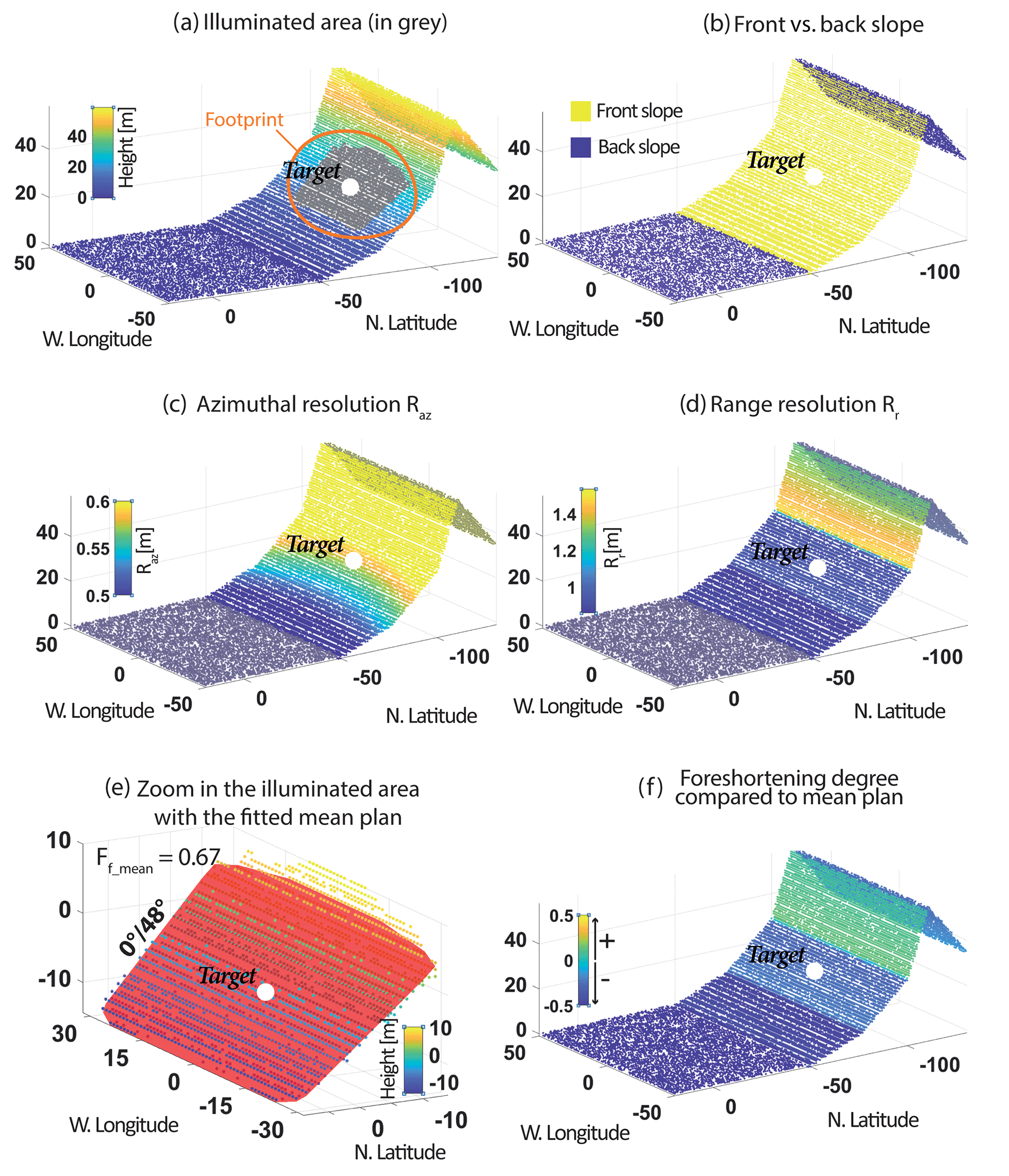
Figure 14 Output maps for the synthetic dataset. (a) Illuminated area and footprint for the chosen parameters. (b) Front vs. back slope. The back slope corresponds to areas in the shadow. (c) The azimuthal resolution increases with the distance to the radar. (d) The range resolution increases with the slope dip, but at the same slope degree, it decreases from the near- to far-range. (e) Zoomed-in view of the illuminated area for which the mean plan is estimated. The mean dip of the area is 48° with a mean foreshortening of 0.67. (f) Foreshortening degree compared to the mean plan F_f-MEAN. Smoother slopes are less affected by the foreshortening than the mean plan. The steeper ones are more affected. The other output maps are presented in Fig. A1.

5.2 Cima del Simano (Figs. 15 and A2)

The LoS distance is almost at the limit of what is acceptable to have for a backscattered signal (3351 m at the target location and 3900 m near the crest). Such a distance decreases the azimuthal resolution considerably, which varies between 8 and 13 m along the range of the illuminated slope (Fig. 15c) for a range resolution of 2.0 m (Fig. 15d). The SoI is affected by a constant and low foreshortening of 0.38 (Fig. 15e and f).

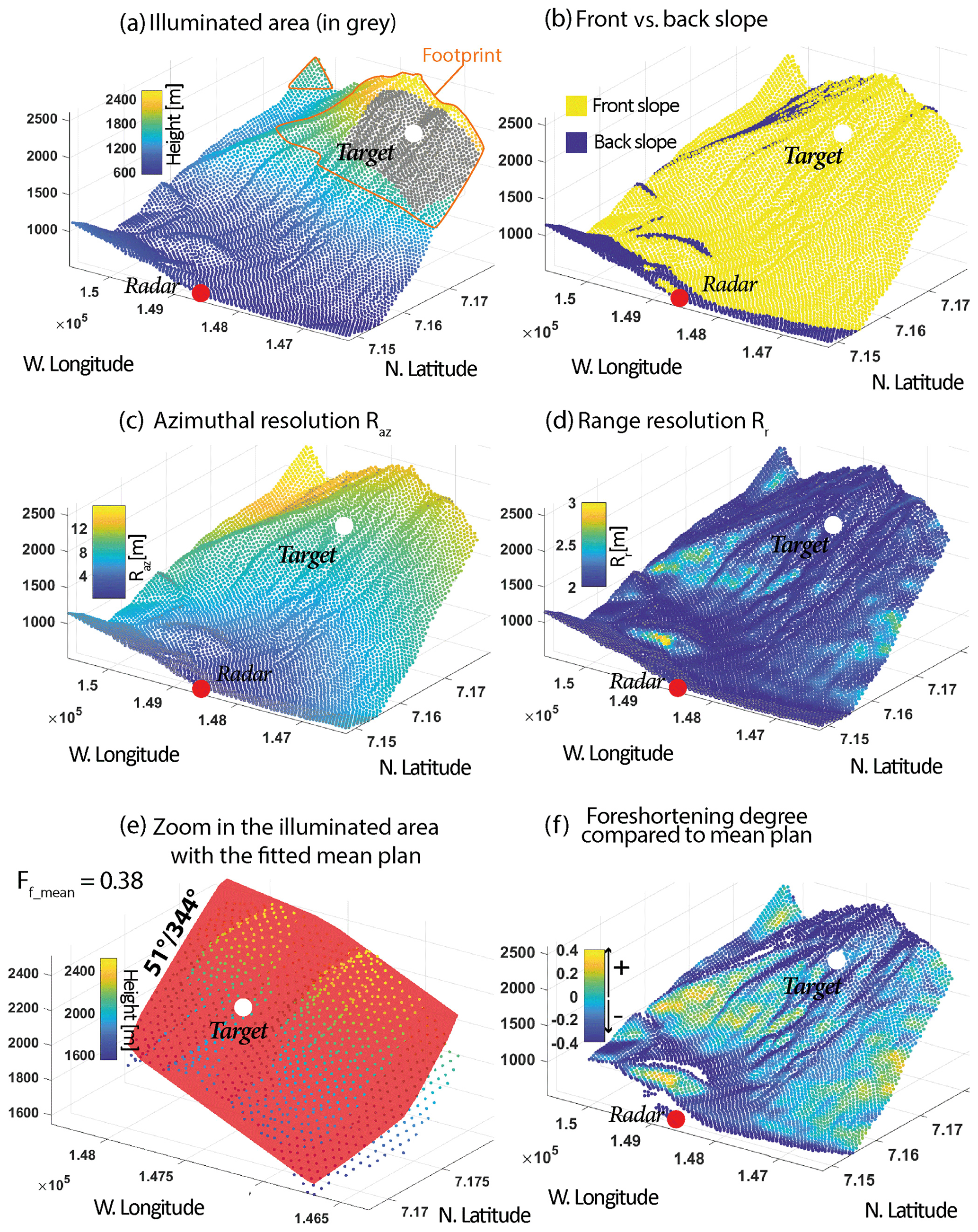
Figure 15 Output maps for the first dataset of Cima del Simano. (a) Illuminated area and footprint for the chosen parameters. (b) Front vs. back slope. The back slope corresponds to areas in the shadow. (c, d) Azimuthal and range resolutions. Since the chosen bandwidth is 75 MHz to be sure to record the backscattered signal, the resolutions are poor. Only a monitoring of the major volume instabilities is relevant here. (e) Zoomed-in view of the illuminated area for which a mean plan fitting is estimated. The mean dip of the area is 51° with a mean foreshortening of 0.38. (f) Foreshortening degree compared to the mean plan. The lower part is more affected by foreshortening at the top of the mountain which is the area of interest. The other output maps are presented in Fig. A2.

5.3 La Cornalle (Figs. 16 and A3)

The LoS distance is 267 m, resulting in a good resolution in the azimuth varying between 0.3 and 0.7 m along the SoI (Fig. 16c) and in the range between 0.8 and 1 m (Fig. 16d). The slope is very steep, and the apparent slope dip is 73°. Consequently, the radar image is affected by a strong foreshortening of 0.81 (Fig. 16e). In the centre of the slope illuminated by the radar (Fig. 16a), one can see a little back slope terrace, which is consequently affected by shadowing (Fig. 16b). The slope below this terrace is less steep than the illuminated area mean plan, oriented $\mathrm{61}/\mathrm{267}$°, while the one located above is steeper. The lower part is less affected by foreshortening than the upper part (Fig. 16f).

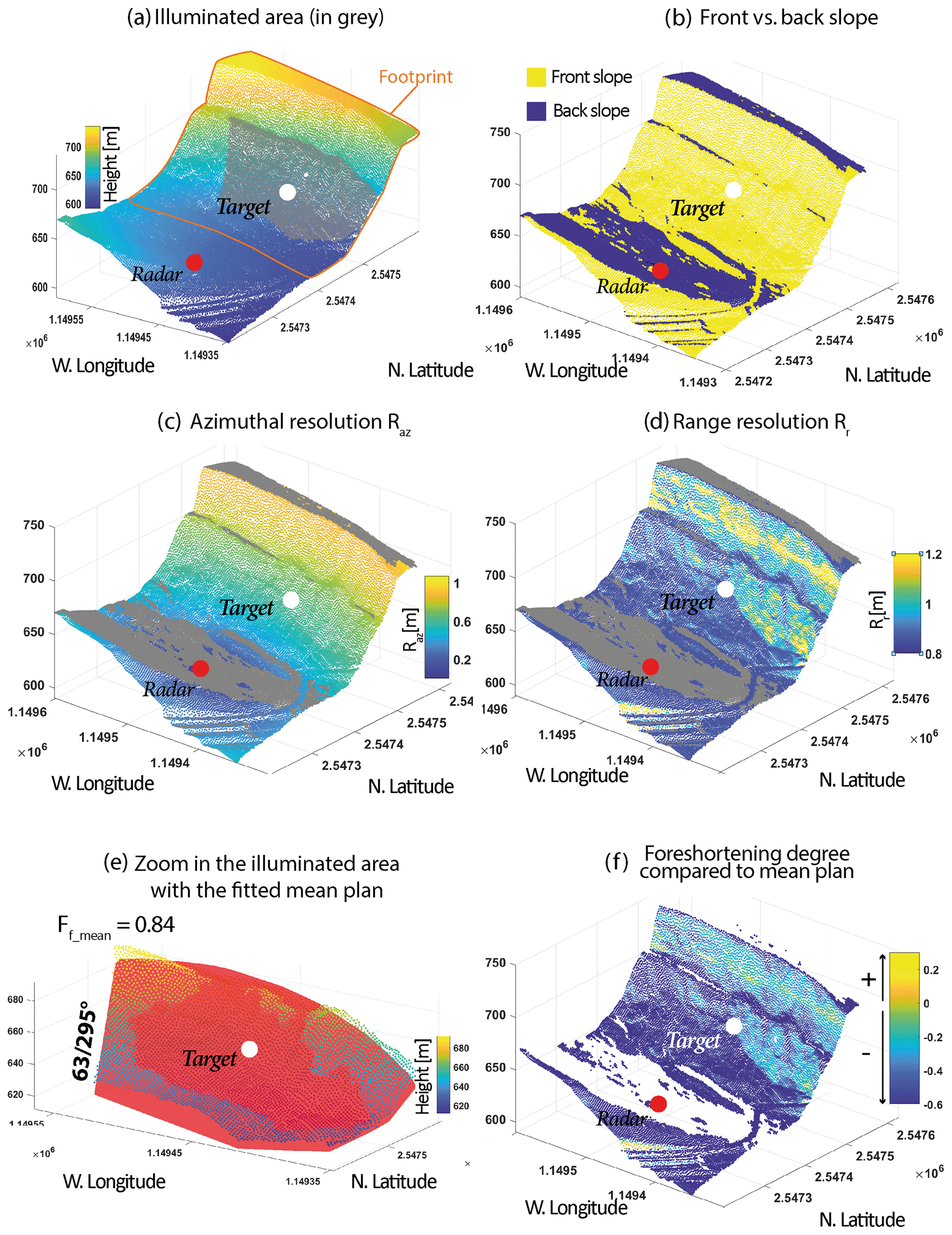
Figure 16 Output maps for the second dataset at La Cornalle cliff. (a) Illuminated area and footprint for the chosen parameters. (b) Front vs. back slope. The back slope corresponds to areas in the shadow. (c, d) Azimuthal and range resolutions. Since the radar is only at a distance of 260 m, the selected bandwidth is 175 MHz to have a good range resolution. (e) Zoomed-in view of the illuminated area for which a mean plan fitting is estimated. The mean dip of the area is 61° with a mean foreshortening of 0.81. (f) Foreshortening degree compared to the mean plan. The other output maps are presented in Fig. A3.

6 Discussion

6.1 Comparison for three different radar locations

Figure 7 presented the impact of the radar location on the resulting image. To verify those concepts, three radar locations, P1, P2 and P3, have been selected at the study site of Cima del Simano to monitor the same region of interest. Their output characteristics are summarized and compared in Table 6. Locations P1 and P2 are located in front of the cliff and along the direction parallel to the slope dip; P1 is further away from the target area than P2. P3 is located almost at the same distance of the cliff as P2 (P3 is 113 m further away from the target than P2) but faces the target area from the side.

Table 6 Comparison of three different radar locations and the impact on their corresponding radar image. Advantages and drawbacks for each position are highlighted.

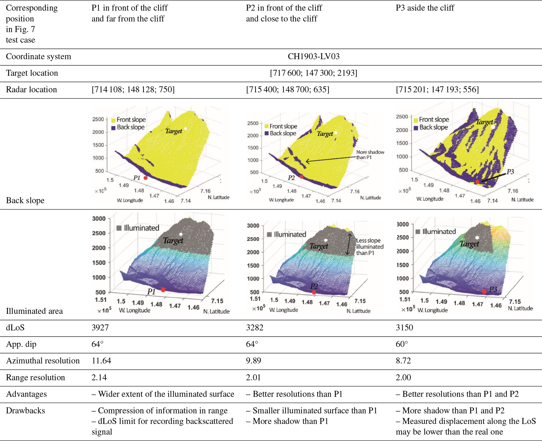
The results are coherent with what is expected from Table 2. An acquisition from P2 gives a better range resolution (2.01 m) compared to P1 (2.14 m). Those two points are located in front of the cliff, and their apparent slope dip corresponds to the real one (64°), while the apparent slope dip for P3 is lower (60°), slightly reducing the range resolution (2.00 m). One could conclude that the best location for the acquisition is P3. Nonetheless, this position triggers more areas in the shadow (back slope), leading to a loss of information. Furthermore, the gravitational movements are often expected to follow the slope dip direction (Dehls et al., 2010; Pedrazzini et al., 2010). Looking at the target area from the side, as with P3, the LoS direction is not parallel to the slope, and the registered displacement may be less than the real one (Colesanti and Wasowski, 2006; Dai et al., 2022).

The illuminated area is wider in the case of P1 than P2 or P3. If the unstable area to monitor is very large, P1 can be advantageous. Since the LoS distance remains smaller than 4 km (3.9 km), the backscattered signal is still registered from P1.

Thus, the best installation location highly depends on the purpose of the acquisition and the area of interest.

• If the main goal is to monitor a large area in order to detect unstable zones and estimate an average displacement rate, such as in Carlà et al. (2019), a position far from the monitored cliff (similar to P1) should be considered. The tool can help check that the LoS distance remains shorter than 4 or 5 km and estimate the extent of the illuminated area. But one must be aware that the resulting range and azimuthal resolutions of the radar will be worse than at location P1.

• If the main goal is to get the best resolution at the expense of the illuminated area size, one should try locating the radar closer to the monitored cliff (similar to P2 and P3). It is the case, for example, when one tries to define the kinematic behaviour (Frattini et al., 2018) or assess the susceptibility of massive rock instabilities to fail (Jaboyedoff et al., 2012). The tool helps check which location (close to , in front of, or aside the cliff) gives the best resolution while avoiding having the SoI in the shadow.

6.2 Tool limitations

Since the input of the program is a DEM converted into a 3D grid, the overhanging slopes, which are those subject to layover, cannot be detected. To overcome this limitation, a suggestion could be to use a point cloud acquired from the ground with a lidar (Abellán et al., 2014) or by photogrammetry (Eltner and Sofia, 2020). But this comes with other problems, such as potential occlusions (Sturzenegger et al., 2007) and noises due to the presence of vegetation which can bias the calculated dip and dip direction of the slope.

7 Conclusion and further development

This paper described the main features of a linear GB-InSAR acquisition, emphasizing and comparing the significant differences from satellite radar acquisitions. While these distinctions are rarely addressed in the literature, they are crucial considerations for anyone initiating a GB-InSAR monitoring campaign.

The paper introduces in a second step a novel MATLAB tool designed for the estimation of the characteristics of linear GB-InSAR acquisitions. This tool generates a set of valuable maps, including the radar-to-target distance, range and azimuthal resolution, foreshortening degree, and shadowing maps in a single operation. The main purpose is to streamline the search for the optimal radar installation site which guarantees the most effective monitoring results when multiple options are considered.

Since the determination of the ideal location varies depending on the objectives of the acquisition campaign, providing comprehensive information critical for selection simplifies the sensitive choice for the most suitable site.

If the purpose is to monitor a large area and to delimitate the unstable zone, then the radar should be installed far from the cliff, using the MATLAB tool to check that the LoS distance remains shorter than 4 or 5 km, depending on the GB-InSAR device. Contrariwise, if the purpose is to characterize the displacement gradient, one will try to optimize the resolution while keeping the LoS as parallel as possible to the displacement vector. In that case, the tool helps verify and avoid the foreshortening and shadowing areas.

Nevertheless, the radar acquisition characteristics are often not the only thing to consider when choosing the best location. Most of the time, the access to electricity and an easy installation on a flat surface, as well as the expected instability movement direction, reduce the choices (Caduff et al., 2015).

The tool could be improved and extended to the other GB-InSARs of type ArcSAR or rotary RAR (Pieraccini and Miccinesi, 2019) and for the estimation of satellite InSAR image characteristics in order to select the best ascending or descending orbit acquisition before starting the downloading and treatment of the images which can also be long and laborious work (Berardino et al., 2002; Mancini et al., 2021).

Appendix A

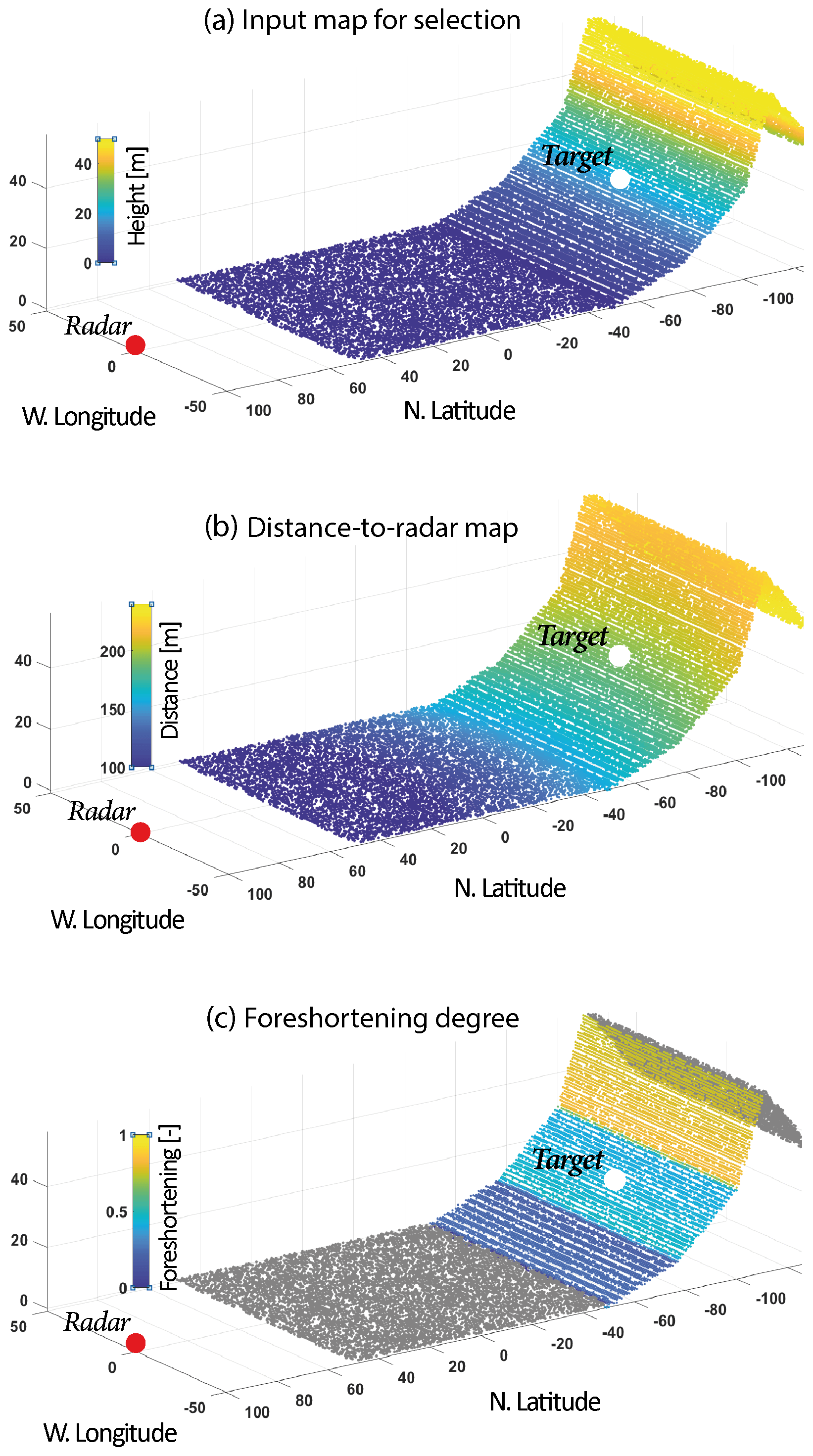
Figure A1 Additional output maps for the synthetic dataset. (a) The input map with the altitude that is aimed at choosing the radar and target location. (b) The distance-to-radar map. The distance between the radar and the target should not be greater than 4 km. (c) The foreshortening map, after Eq. (8).

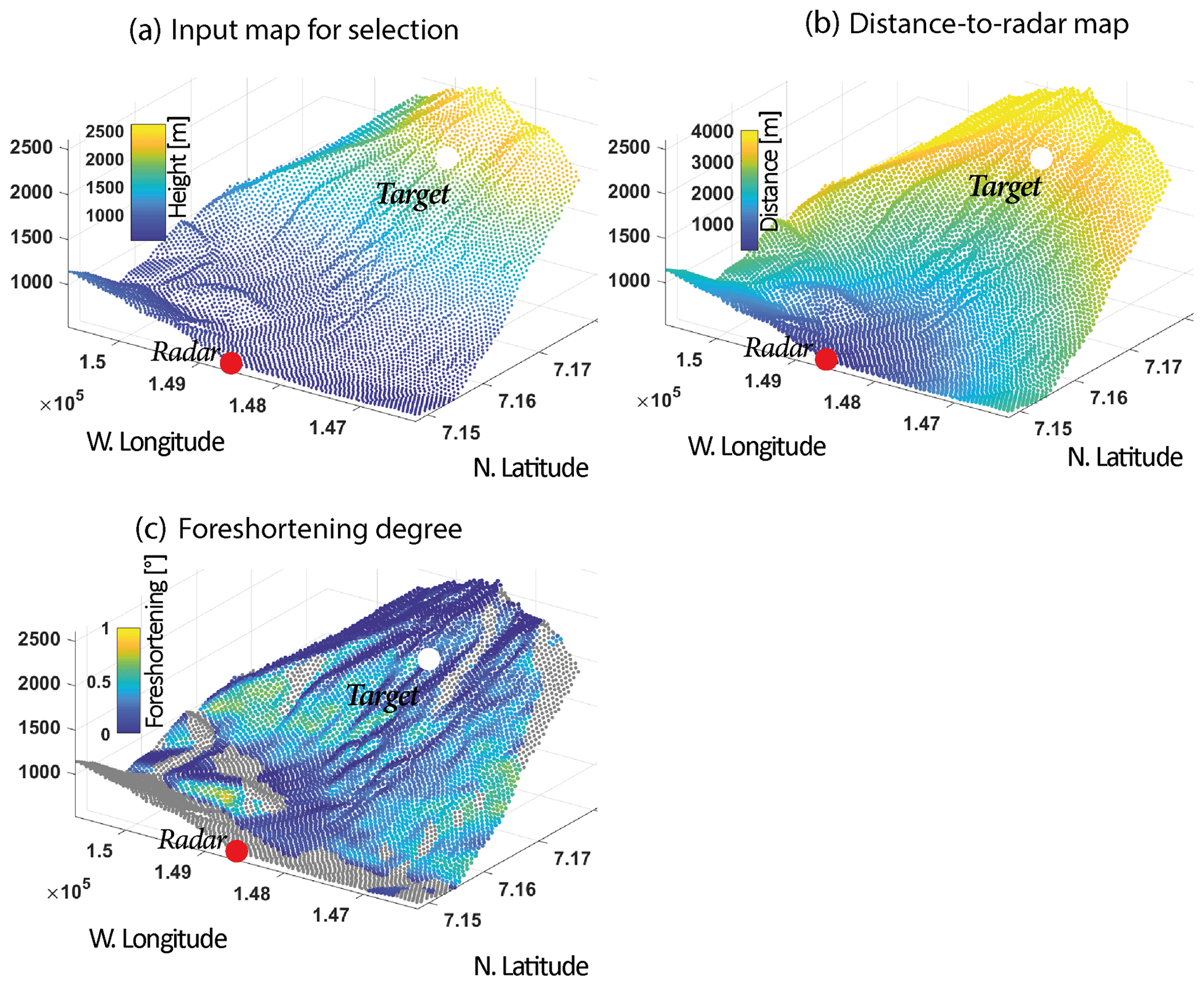
Figure A2 Additional output maps for the first real dataset; Cima del Simano. (a) The input map with the altitude is aimed at choosing the radar and target location. (b) The distance-to-radar map. The distance between the radar and the target should not be greater than 4 km. (c) The foreshortening map, after Eq. (8).

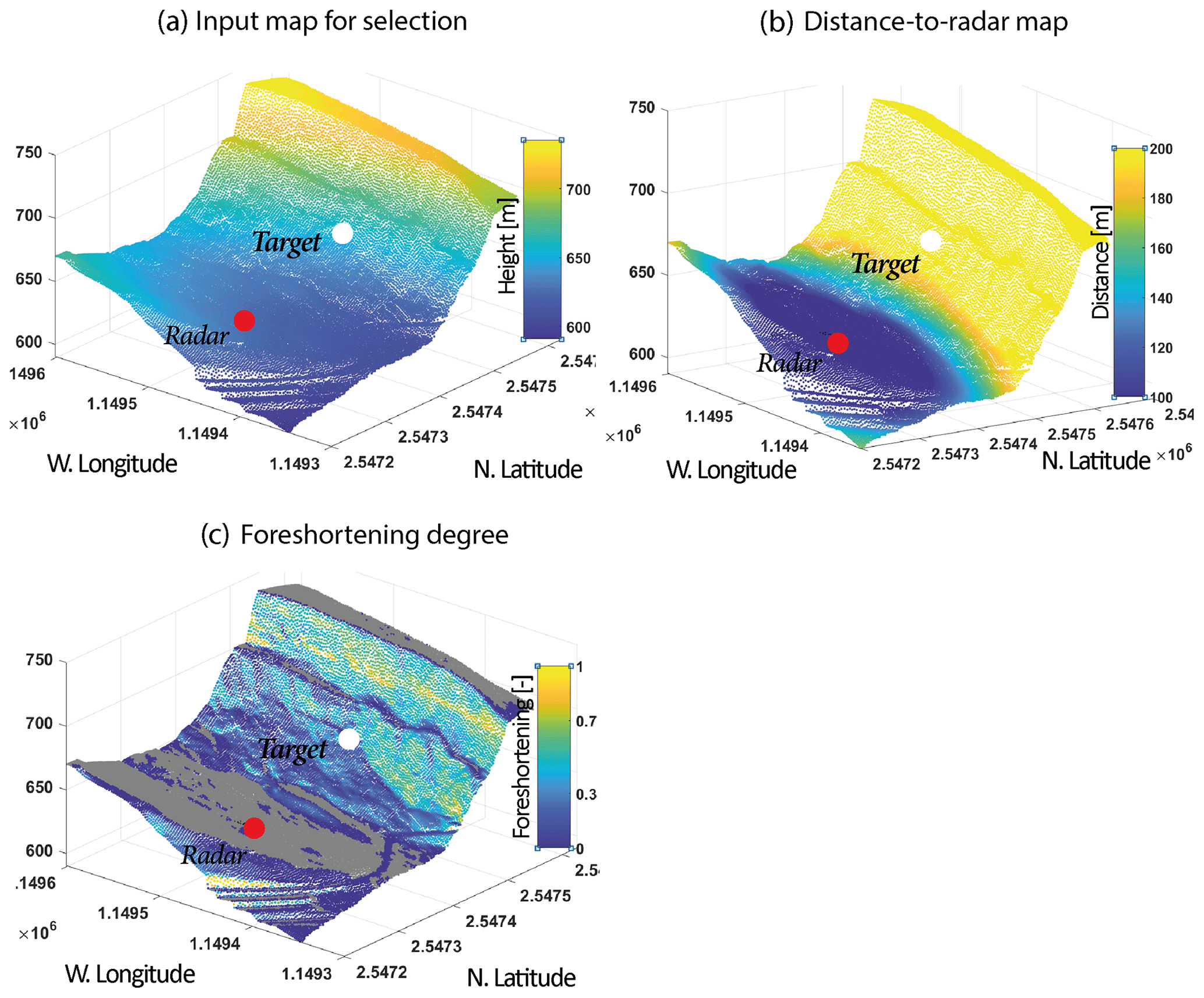
Figure A3 Additional output maps for the second real dataset; La Cornalle. (a) The input map with the altitude is aimed at choosing the radar and target location. (b) The distance-to-radar map. The distance between the radar and the target should not be greater than 4 km. (c) The foreshortening map, after Eq. (8).