A free, open-source method for automated mapping of quantitative mineralogy from energy-dispersive X-ray spectroscopy scans of rock thin sections

Quantitative mapping of minerals in rock thin sections delivers data on mineral abundance, size, and spatial arrangement that are useful for many geoscience and engineering disciplines. Although automated methods for mapping mineralogy exist, these are often expensive, associated with proprietary software, or require programming skills, which limits their usage. Here we present a free, open-source method for automated mineralogy mapping from energy-dispersive spectroscopy (EDS) scans of rock thin sections. This method uses a random forest (RF) machine-learning image classification algorithm within the QGIS geographic information system and Orfeo ToolBox, which are both free and open-source. To demonstrate the utility of this method, we apply it to 14 rock thin sections from the well-studied Rio Blanco tonalite lithology of Puerto Rico. Measurements of mineral abundance inferred from our method compare favorably to previous measurements of mineral abundance inferred from X-ray diffraction and point counts on thin sections. The model-generated mineral maps agree with independent, manually delineated mineral maps at a mean rate of 95 %, with accuracies as high as 96 % for the most abundant mineral (plagioclase) and as low as 72 % for the least abundant mineral (apatite) in these samples. We show that the default random forest hyperparameters (i.e., tuneable settings that control behavior) in Orfeo ToolBox yielded high accuracy in the model-generated mineral maps, and we demonstrate how users can determine the sensitivity of the mineral maps to hyperparameter values and input features. These results show that this method can be used to generate accurate maps of major minerals in rock thin sections using entirely free and open-source applications.

1 Introduction

Minerals are the fundamental units of rocks and many engineered materials (Perkins, 2020; Callister and Rethwisch, 2020). Improving the quantification of mineral properties is a long-standing research objective in industry and academic research (Pirrie and Rollinson, 2011), given the importance of mineral properties in chemical weathering (e.g., Hilton and West, 2020), rock damage (e.g., Shen et al., 2019; Xu et al., 2022), planetary evolution (e.g., Hazen et al., 2008), crustal deformation (e.g., Burgmann and Dresen, 2008), and nutrient supply (e.g., Callahan et al., 2022). Quantitative automated mineralogy, the computerized mapping of minerals across a sample, results in measurements of mineral modal abundance, mineral grain size and shape, and the spatial arrangement of minerals amongst one another (Sutherland et al., 1988; Sutherland and Gottlieb, 1991; Gu, 2003; Schulz et al., 2020). Modal abundance is useful because it can yield information on the sedimentary and tectonic environments in which the rock formed (Harlov et al., 1998; Hupp and Donovan, 2018), while the spatial arrangement of minerals in a rock, termed rock fabric, can yield further data on mechanical anisotropy and paleo-environmental conditions during the rock's formation and metamorphism (Přikryl, 2006; Bjørlykke, 2014). Simultaneous quantification of modal mineralogy and detailed mapping of the spatial arrangement of minerals in an automated manner, or automated mineralogy, is thus a key tool for investigating many geologic processes. Wide adoption of automated mineralogy techniques is limited by the prohibitive cost or programming skills required to use many automated mineralogy software applications, so this technique has mostly been restricted to ore characterization, resource processing, and petroleum geology (Nikonow and Rammlmair, 2017; Schulz et al., 2020).

In practice, automated mineralogy methods use a combination of image analysis and classification methods to identify minerals from elemental composition data (or their derivatives), which can be collected with a variety of analytical methods, including energy-dispersive X-ray spectroscopy (EDS), micro-X-ray fluorescence (µ-XRF), and laser-induced breakdown spectroscopy (LIBS) (Nikonow et al., 2019). Automated mineralogy is slowly being adopted by researchers outside of resource extraction for combined modal analysis of bulk mineralogy, estimates of grain size distribution, and mineral association (Han et al., 2022), which can be useful in a variety of disciplines such as petrology, applied geochemistry, and rock mechanics (Sajid et al., 2016; Elghali et al., 2018; Rafiei et al., 2020).

Automated mineralogy from EDS with the aid of back-scattered electron (BSE) imaging has been developing since the 1980s and has grown alongside advances in scanning electron microscopy (SEM) and image processing algorithms (Miller et al., 1983; Fandrich et al., 2007). Commercial automated mineralogy systems are available as integrated hardware–software systems or as standalone software packages which are combined with scanning electron microscopes (Schulz et al., 2020). Some systems only work with certain scanning electron microscopes and detectors from the same company, such as QEMSCAN (Gottlieb et al., 2000), FEI-MLA (Fandrich et al., 2007), and TESCAN TIMA-X (Hrstka et al., 2018). Others are purely software-based solutions which are integrated with various SEMs: ZEISS Mineralogic, Oxford AZtecMineral, and Thermo-Scientific MAPS Mineralogy. The price of hardware and software upgrades required to accommodate these systems renders them cost-prohibitive to many labs outside the resource extraction industry (Nikonow and Rammlmair, 2017). All systems have some general ability to classify EDS spectra based on a database of predefined and/or customizable mineral spectra standards (Schulz et al., 2020). Since the underlying software is proprietary, no source code is available for these systems, and details on how they use spectra to classify minerals are sparse to non-existent (Kuelen et al., 2020). Furthermore, the accuracy of mineral prediction from these systems has rarely been quantified (Blannin et al., 2021).

To date, several open-source (i.e., source code is available and modifiable) automated mineralogy solutions have been implemented. Ortolano et al. (2014, 2018) predicted modal mineralogy and mapped minerals from a multistep workflow involving principal component analysis, maximum likelihood classification, and multi-linear regression performed on EDS or WDS (wavelength-dispersive X-ray spectroscopy) spectral data using the Python extension within ArcGIS. Li et al. (2021) used a variety of legacy machine-learning and deep-learning models to classify minerals in oil reservoir rocks using mineral maps generated from proprietary software as training data. In terms of image classification, deep-learning methods are state of the art but currently require the user to be relatively adept at programming and knowledgeable of the computer vision principles employed (Khan et al., 2018; Zhang et al., 2019). A method that requires little to no programming ability would allow more users to benefit from automated mineralogy data. An example of this approach is XMapTools by Lanari et al. (2014), a graphical, open-source automated mineralogy solution with multiple machine-learning classification algorithms within a standalone MATLAB-based environment.

Random forest (RF) classification is a supervised classification algorithm (i.e., the user generates training data) in which an ensemble of decision trees produces a majority vote that assigns a thematic classification to unknown data (Breiman, 2001). Each decision tree within the ensemble is trained on a random sample of the training data using only a set number of random features at each branch (Cutler et al., 2011). During prediction, for each decision tree, unknown data traverse a sequence of rule-based branches which culminate in the assignation of a predicted class (Breiman, 2001). Each tree gets one vote for each pixel; the predicted class with the most votes is assigned to the unknown data. There are several reasons why RF classification is useful for automated mineralogy mapping. It is well suited for accommodating unbalanced training data and nonparametric data distributions (Maxwell et al., 2018), which are common in rock samples due to large differences in relative mineral abundances and elemental intensities (Ahrens, 1954). In addition, recent work showed that RF classification performed better than other legacy machine-learning algorithms (e.g., support vector machines; Hearst et al., 1998) in mineral classification of reservoir rocks (Li et al., 2021).

The main goal of this study is to present a new, user-friendly quantitative automated mineralogy method that we developed and implemented within QGIS, a free and open-source geographic information system. Unlike previous methods, the method presented here uses only freely available and open-source applications, and it requires no programming by the user. We use the free and open-source Orfeo ToolBox plugin for QGIS (Grizonnet et al., 2017) to predict thin-section-scale bulk mineralogy from EDS elemental intensity data using an RF image classifier (Breiman, 2001). Situating the workflow within a GIS environment has advantages over standalone programs such as direct access to raster and vector manipulation and analysis tools and database management (Tarquini and Favalli, 2010; Berrezueta et al., 2019). Furthermore, we present an overview of the automated mineralogy method and apply it to a set of rock samples from the Rio Blanco tonalite to demonstrate the method's utility. By outlining an easy-to-use and open-source solution, we intend to provide an automated mineralogy method to a broader community of users.

2 Overview of the method

The goal of our automated mineralogy method is to produce quantitative mineralogy maps of rock thin sections solely from EDS data acquired using an SEM. Here, in Sect. 2, we briefly summarize each step needed to reach a predicted mineral map. In Sect. 3, we demonstrate how to use the method by applying it to a set of rock thin sections, during which we elaborate on the choices users need to make and the functions they need to use during each step. We also provide a detailed step-by-step guide in the Supplement (Reed et al., 2024).

The starting point for this method is elemental rasters derived from EDS-generated scans of rock thin sections. For the purposes of our method, we take these scans as already measured and in hand. Generating such scans requires preparing thin sections and analyzing them with a scanning electron microscope, both of which are done by established procedures (Goldstein et al., 2018). The necessary output from such scans are rasters of elemental intensity (counts eV⁻¹), one for each element of interest (e.g., Ca, Na, K). After the EDS elemental intensity rasters have been generated, all the remaining steps in the method are conducted in QGIS. No programming is required in any step. Instead, users need only be familiar with QGIS and their samples.

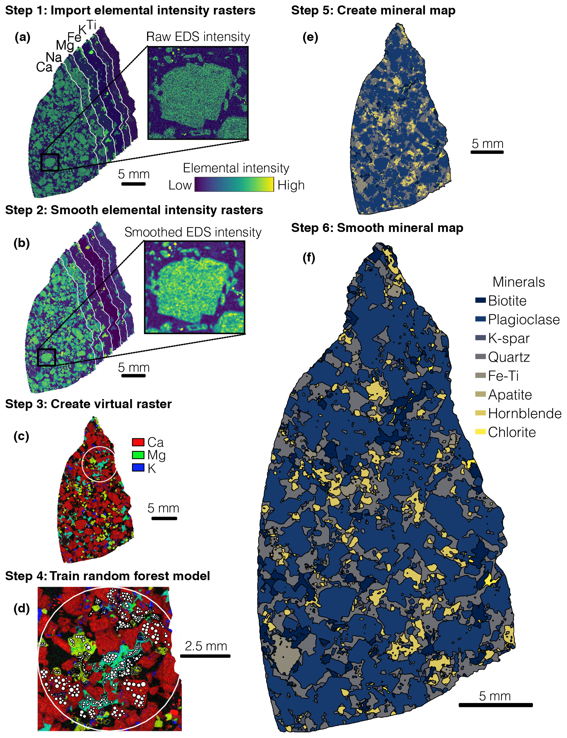
Figure 1 Example application of the automated mineralogy method. (a) Step 1: import raw elemental intensity rasters (Ca, Na, Mg, Fe, K, and Ti) into QGIS. Here, the rasters shown are for the thin-section sample 1-13a. The zoomed-in view of the Ca raster exemplifies the short-wavelength noise in the elemental rasters. (b) Step 2: smooth each elemental intensity raster with a circular mean filter. The zoomed-in view shows that this filter has eliminated much of the short-wavelength noise that was in the raw elemental rasters. (c) Step 3: create a virtual raster by combining the smoothed elemental rasters into a single image container with bands for each element. The white circle shows the area within which polygons were generated to train the random forest (RF) model in Step 4. (d) Step 4: within the training area boundary in the virtual raster (large white circle, as in Step 3), draw a series of small polygons (here, small white circles). Each polygon must lie within a single known mineral, and collectively these small polygons must sample all minerals of interest (here, plagioclase feldspar, quartz, hornblende, biotite, potassium feldspar, Fe–Ti oxides, apatite, and chlorite). These polygons collect the pixel-level data on which the RF model will be trained. (e) Step 5: apply the trained RF model to the entire sample to create a thin-section-scale mineral map. (f) Step 6: smooth the RF-predicted mineral map with a circular majority filter.

The first step involves importing the raw elemental intensity rasters into QGIS with no coordinate reference system (Fig. 1a). This also involves compiling a list of all the minerals that will be mapped in the thin section, which can be assessed based on prior knowledge, literature, and examination of EDS spectra. Our method is not viable for those thin sections from completely unknown lithologies that resist efforts to identify minerals under the microscope and/or manual examination of EDS data. As we describe in Sect. 4, we recommend restricting this to minerals with sufficiently high abundance (>0.1 %) to be adequately trained upon. For those workers that require high accuracy in very low abundance minerals, our method is not advisable.

The second step is to smooth the raw elemental intensity rasters (Fig. 1b). This is useful because EDS-generated elemental intensity rasters are subject to noise, which can arise through electron beam interactions with the sample (Goldstein et al., 2018). As we describe in Sect. 4.3, we found that this smoothing step was best done with a 7-pixel-radius circular mean filter, in which each pixel is assigned the mean value of the surrounding pixels in a circular window (Gonzalez and Woods, 2018). We performed this on intensity rasters from the example samples to which we applied our method in Sect. 3. For this, we used the free and open-source System for Automated Geoscientific Analyses (SAGA) plugin for QGIS (Conrad et al., 2015).

The third step is to gather the smoothed elemental intensity rasters into a virtual raster, a type of container for multiple rasters, with one band for each element of interest (Fig. 1c). For example, if the user chooses to import elemental intensity rasters for six elements, as we did in the application of this method to our samples in Sect. 3, this will result in a virtual raster with six bands. For this, we used the Geospatial Data Abstraction Library (GDAL/OGR contributors, 2022), which is a standard library in QGIS.

The fourth step is to train an RF image classification model on the virtual raster (Fig. 1d). This requires generating a large number (∼ hundreds) of small polygons on the virtual raster. Each of these small polygons must lie within a single mineral, which the user must identify and assign to the polygon. Collectively, these small polygons must cover all the minerals of interest in the thin section in sufficient number to train the RF model. If the user wishes to assess the accuracy of the RF-predicted mineral map to a manually mapped portion of the thin section, we recommend restricting the location of these small training polygons to a relatively small portion of the thin section (∼10 %–20 % by area). This will ensure that other portions of the thin section can be mapped manually to compare against the RF-predicted mineral map. If the user does not wish to conduct such an accuracy assessment after the RF-predicted mineral map is complete, then these small training polygons can be generated anywhere across the entire thin section.

After the RF model has been trained, the fifth step is to apply the trained RF model to the entire virtual raster (Fig. 1e). During this step, the RF model assigns a mineral class to every pixel in the virtual raster, which yields a mineral map for the entire thin section. For these RF modeling steps, we used the free, open-source Orfeo ToolBox plugin for QGIS (Grizonnet et al., 2017).

The sixth and final step is to denoise the RF-generated mineral map (Fig. 1f). For this, we applied a circular majority filter using the SAGA plugin for QGIS, in which each pixel is assigned the modal value of the surrounding pixels in a circular window (Gonzalez and Woods, 2018). As we describe in Sect. 4.3, we found that this was best done with a 10-pixel-radius majority filter in the example samples to which we applied this in Sect. 3. This eliminates most isolated pixels within larger groups of pixels of a uniform predicted mineral and rare pixels that were not classified due to voting ties (Ortolano et al., 2018; Nikonow et al., 2019)

At this stage, the RF-predicted mineral map is complete. It can now be examined or manipulated according to the user's needs. For instance, the mineral map can be converted from a raster to a vector form to facilitate the measurement of mineral grain size and other properties (Sect. 5.2).

3 Application of the method

3.1 Preparation of rock thin sections from the Luquillo Critical Zone Observatory

To demonstrate the utility of the method described in Sect. 2, we applied it to 14 thin sections of Rio Blanco tonalite from the Luquillo Critical Zone Observatory (LCZO) in Puerto Rico, United States, a site that has been the subject of substantial research on the weathering of igneous rocks into saprolite and soil (White et al., 1998; Riebe et al., 2003; Stallard and Murphy, 2012; Brocard et al., 2023). The lithology is a phaneritic, plutonic igneous rock with some evidence of low-grade hydrothermal alteration (Speer, 1984). The Rio Blanco tonalite provides an ideal case study because mineral abundance has been characterized previously via quantitative X-ray diffraction (XRD) and point-counting modal analysis (i.e., systematic manual identification and counting under microscope; Ingersoll et al., 1984), which indicated the rock consists of plagioclase feldspar (andesine), quartz, biotite, hornblende, potassium feldspar, magnetite, apatite, and chlorite (Murphy et al., 1998; Buss et al., 2008; Ferrier et al., 2010).

To ready the samples for EDS, 14 petrographic thin sections were prepared on 27×46 mm glass slides from bedrock core quarters collected from the Rio Icacos catchment within the LCZO (Comas et al., 2019). The samples ranged in area from 34.7 to 139.5 mm². Four samples are composed of weathered rock nearer to the surface, while the rest are more pristine bedrock (Orlando et al., 2016). From each core depth, two thin sections were prepared in vertical and horizontal orientations. Our own preliminary optical microscopy observations revealed that these samples contained abundant plagioclase, quartz, hornblende, and biotite, which is consistent with previous modal analyses (Murphy et al., 1998; Buss et al., 2008).

3.2 Measuring elemental intensity in thin sections with energy-dispersive spectroscopy

Each thin section was mapped with energy-dispersive X-ray spectroscopy (EDS) using a Hitachi S-3400 VP-SEM with a thermionic tungsten electron source equipped with an Oxford Instruments X-Act 10 mm² silicon drift detector receiving X-rays across 2048 spectral bands. The EDS detector acquires a spectrum showing the energy and intensity of characteristic X-rays emitted from the sample to determine the atomic composition of the sample within the analysis volume of the primary beam (Goldstein et al., 2018). For the measurements on our thin sections, the instrument and accompanying software produced full thin-section elemental intensity maps (counts eV⁻¹) at a resolution of 4 µm pixel⁻¹, which was determined by the beam step size. EDS data were acquired with an accelerating voltage of 15 kV and a beam current of ∼10 nA. The EDS process time (also known as “time constant” by some manufacturers) was 4, which is an intermediate value that balances acquisition time and data quality. EDS acquisition time was ∼3.5 h for each thin section.

From the EDS analysis application included with this instrument (AZtec), we exported six TIF files for each sample (Fig. 1a) consisting of full-resolution elemental intensity rasters for the elements of interest (Ca, Na, K, Mg, Fe, and Ti). These rasters contain the X-ray counts of elemental intensity at each pixel and have a mean size of over 20 megapixels over the 14 studied thin sections. We selected these elements because they are present in varying abundance in the minerals within the Rio Blanco tonalite and hence are useful for distinguishing among the minerals in these samples. For example, K, Mg, Fe, and Ti are present at high abundance in biotite (Dong et al., 1999) but are present at low abundance in other major minerals in this lithology (e.g., plagioclase feldspar, quartz). Our initial attempts at classification showed that the inclusion of rasters of Si and Al had no effect on classification accuracy, so we did not include them here.

This method requires a list of minerals present in the samples for both training of and prediction by the RF models (steps 4 and 5 in Sect. 2). Such a list can be obtained in a variety of ways, including prior studies of qualitative mineralogy of the host lithology or mineral identification from optical microscopy on the sample thin sections. For the 14 samples analyzed here, we generated a list of minerals by inspecting the EDS-generated X-ray spectral data within Oxford AZtec, a proprietary software package integrated with the SEM that we used to measure EDS scans of our samples. From these spectra, we identified plagioclase feldspar, quartz, hornblende, biotite, potassium feldspar, Fe–Ti oxides (predominantly magnetite–titanomagnetite), and apatite as mineral classes for the RF models (Sect. 3.3). For those without offline access to a full EDS environment, some systems such as Oxford AZtec allow the full export of data into text or binary formats, which can be accessed with free and open-source tools (e.g., HDFView or NIST DTSA-II). Due to trace abundance (Murphy et al., 1998), other minerals present in the samples, such as epidote and titanite, lacked an adequate number of trainable examples, so they were neglected or combined with an associated mineral, Fe–Ti. For reference, the mean abundance of apatite, the lowest-abundance mineral we trained, was ∼0.1 %. We recommend that minerals present at abundances lower than this be omitted or combined with the understanding that overall accuracy is most likely being negatively impacted in a minor way.

3.3 Smoothing and virtualization of the elemental intensity rasters

We smoothed each elemental intensity raster with a 7-pixel-radius circular mean filter using SAGA's Simple Filter tool to eliminate noise in the EDS data. We chose this filter size because it optimized the accuracy calculated during the training and validation of the RF model. We test the sensitivity of this choice in Sect. 4.3. We then used the GDAL gdalbuildvrt command within QGIS to group the smoothed elemental intensity rasters into a virtual raster dataset, in which each elemental raster is represented as a separate band. A virtual raster is a container for multiple rasters that encodes metadata such as file locations and other attributes in extended markup language (XML) (McInerney and Kempeneers, 2014). Opening and processing virtual raster datasets requires fewer computer resources, as the underlying rasters are only accessed when required.

3.4 Training random forest models for mineral classification

Before an RF model can be tasked with assigning a mineral class to every pixel in an entire thin section, it must first be trained upon the minerals in the thin section. On each of the virtual rasters for the 14 thin sections, we selected an area encompassing less than ∼15 % of the total thin-section sample area within which we trained the model. We selected training areas that represented all minerals as well as possible so that each mineral would receive an adequate amount of training data for each mineral. Selecting a small training area in the thin section is useful because it enables users to test the accuracy of the trained model on other areas of the thin section, if desired. This is not a necessary step in the method, but in Sect. 4 we show how such accuracy tests can be done on other portions of the thin sections.

For each mineral within the training area, we manually generated hundreds of circular polygons upon the virtual raster using the knowledge gained previously from examining the EDS spectra (Fig. 1). A single training polygon within the training area collects all pixel values contained within it from each elemental intensity raster composing the virtual raster. Labeling this polygon as a single mineral effectively labels every pixel value contained within it as that mineral. We note that, during this training step, the user should take care not to misidentify or neglect training upon abundant minerals, which could have a detrimental effect on the classification accuracy. To prevent this outcome, we used all available elemental rasters to verify that training polygons were within the bounds of the identified mineral. For a few thin sections, multiple subareas composed the training area to incorporate enough data on less abundant minerals such as apatite. Because each training polygon encompassed pixel-level data for all bands from the virtual raster, the training datasets were large (>10⁵ pixel-level samples for each thin section). Hundreds to thousands of pixel-level training samples per class are generally considered sufficient for RF models (Cutler et al., 2012). Training samples per mineral were highly unbalanced (i.e., some minerals covered many more pixels than others) due to the high abundances of quartz and plagioclase relative to those of a minor mineral such as apatite. Orfeo ToolBox handles this potential problem automatically by randomly selecting samples at a rate relative to the size of the smallest class, ensuring that the minority classes such as apatite have an equal probability of being drawn into a sample subset used to construct an individual decision tree.

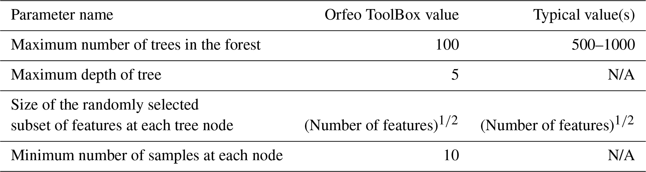
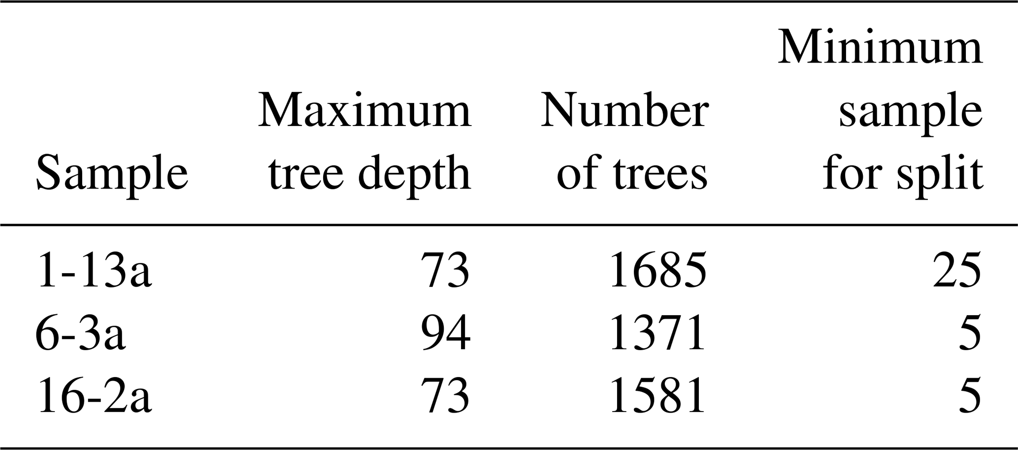
Using the training data obtained from the virtual raster for each thin section, we trained RF image classification models using the TrainImagesClassifier function in Orfeo ToolBox. In this function, users must select hyperparameter values for the RF model, which are tuneable parameters that control model behavior. In machine learning, hyperparameters define the general behavior of a model and are distinct from model parameters, which are learned through training. For more details about RF machine-learning model hyperparameters, see the review in Probst et al. (2019). We used the default hyperparameter values pre-selected in Orfeo ToolBox (Table 1) for the models employed for our final predicted mineral maps.

A measure of model accuracy is automatically calculated by the TrainImagesClassifier function at this step using unseen training data, which can be useful to examine before proceeding so as to ensure that the RF model is operating correctly. The accuracy metric we focus on in this study is the F1 score (Eq. 3), which is the harmonic mean of the precision metric (Eq. 1) and the recall metric (Eq. 2). This is a useful measure of the accuracy of RF-predicted minerals because it penalizes false positives and false negatives while rewarding true positives and neglecting true negatives (Chinchor and Sundheim, 1993), which can be very plentiful for low-abundance minerals:

$$\begin{array}{}\text{(1)}& {\displaystyle }\mathrm{precision}={\displaystyle \frac{\mathrm{true}\mathrm{positives}}{\mathrm{true}\mathrm{positives}+\mathrm{false}\mathrm{positives}}},\text{(2)}& {\displaystyle }\mathrm{recall}={\displaystyle \frac{\mathrm{true}\mathrm{positives}}{\mathrm{true}\mathrm{positives}+\mathrm{false}\mathrm{negatives}}},\text{(3)}& {\displaystyle }\mathrm{F}\mathrm{1}\mathrm{score}={\displaystyle \frac{\mathrm{2}\left(\mathrm{precision}\right)\left(\mathrm{recall}\right)}{\mathrm{precision}+\mathrm{recall}}}.\end{array}$$

In the application of Eqs. (1)–(3) to mineral maps, a true positive is defined as pixel-level agreement on the presence of a given mineral between the model prediction and unused training data, which the algorithm holds out from training for the purpose of calculating metrics such as the F1 score. Similarly, a true negative is agreement on the absence of a given mineral class. False positives and false negatives are disagreements on the presence and absence of a given mineral class, respectively. Application of the default hyperparameters to our samples yielded very high F1 scores (∼0.99). This gave us confidence that the predicted mineral maps generated using the default hyperparameters were near optimal for comparison with manually delineated test maps (described in Sect. 4.1).

Table 1 Default hyperparameter values for the Orfeo ToolBox RF machine-learning model and typical values according to Probst et al. (2019).

We applied each trained model to its corresponding virtual raster to predict a single mineral class at each pixel, except in the case of ensemble voting ties, in which case no mineral class was assigned to that pixel. This resulted in mineral maps at the same resolution as the virtual rasters (∼4 µm).

3.5 Using the random forest models to generate mineral maps

In our application of the trained RF models to our thin sections, the models calculated the entire thin-section-scale mineral maps in a under 1 min using a desktop computer (4 GHz processor, 64 GB memory). Figure 1 shows an example of one of these mineral maps.

After a thin section's mineral map has been generated, it is trivial to calculate the abundance of each mineral by counting pixels. Figure 2 shows the abundance of each mineral across all 14 samples with the error given by the mean F1 scores of the minerals. It also reveals relatively little variation in each mineral's abundance among the 14 samples, which is consistent with previous observations of the Rio Blanco tonalite. The RF-predicted mineral abundances compare well with those measured from modal analysis via point counting on BSE imagery (Buss et al., 2008) and via quantitative XRD (Ferrier et al., 2010). Buss et al. (2008) measured average areal abundances of 19.9 % and 49.3 % for quartz and plagioclase, respectively, comparable to the RF-predicted average abundances of 22.8±1.0 % and 55.8±2.3 % (± error from mean F1 scores) on our 14 thin sections. The combined abundance of hornblende and biotite (“Fe-silicates”) measured by Buss et al. (2008) was 24 %, which is close to the maximum RF-predicted abundance of “Fe-silicates” among our 14 samples (25.0±1.5 %). Using common values for molar masses (M mol⁻¹) and densities (M L⁻³), the XRD-based abundances (converted to areal abundance) from Ferrier et al. (2010) for quartz, plagioclase, and hornblende were 24 %, 62 %, and 14 %, respectively, while the RF-predicted mineral maps yielded 22.8±1.0 %, 55.8±2.3 %, and 10.4±0.7 %, respectively. When quartz, plagioclase, and alkali feldspar abundances are normalized for usage with a quartz–alkali feldspar–plagioclase–feldspathoid diagram (Le Maitre, 2002), the RF-predicted abundances for each mineral demonstrated that all thin sections can be classified as tonalite, matching the name of the lithology.

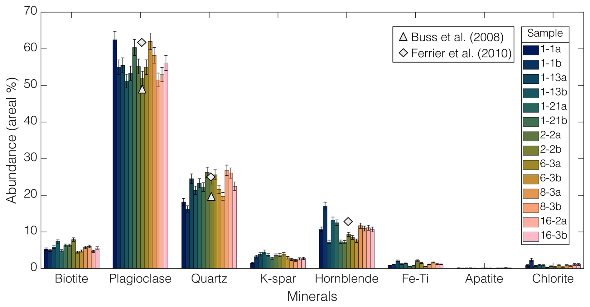
Figure 2 Areal abundance for all 14 samples of the Rio Blanco tonalite. Error bars stem from mean F1 scores for each individual mineral from test map comparisons (see Sect. 4.1). Data from the analyses of the Rio Blanco tonalite in Buss et al. (2008) and Ferrier et al. (2010) are included for reference.

4 Discussion: accuracy of random-forest-predicted mineral maps and sensitivity analyses

4.1 Accuracy of random-forest-predicted mineral maps

Before applying the trained RF models to the full thin sections, we manually mapped the mineralogy of a small section for three representative samples (6-3a, 16-2a, and 1-13a) to assess the accuracy of the model-generated mineral maps. We refer to these manually delineated mineral maps as “test maps”. These test maps were manually delineated as vector polygons for all mineral classes using the elemental intensity rasters for guidance. For example, when mapping a grain of potassium feldspar, we determined the boundaries of the grain with filtered and unfiltered rasters of K and combined intensity rasters of multiple elements. We consider these maps to be “ground truth” data, which are never perfect representations of reality (Foody, 2024) but, nonetheless, may serve to compare the performance of this method to the extremely slow process of manually mapping grain boundaries. We then rasterized the manually delineated vector maps, which resulted in the classification of every pixel within the test maps as one of the eight minerals. The test maps averaged over 1 million pixels in size.

We compared the same section of the predicted mineral maps to the test maps using a frequency-weighted F1 score (Eq. 4) to gauge the average accuracy for all mineral classes. To calculate a frequency-weighted F1 score, the F1 score for the ith class (F1 score_i) is weighted by the class frequency (w_i), which is the proportion of pixels of class i to the total number of pixels in the test map. Here, N is the number of mineral classes:

$$\begin{array}{}\text{(4)}& \mathrm{frequency}\text{-}\mathrm{weighted}\mathrm{F}\mathrm{1}\mathrm{score}={\sum }_{i=\mathrm{1}}^N{w}_i\mathrm{F}\mathrm{1}{\mathrm{score}}_i.\end{array}$$

We clipped the portion of the predicted mineral map overlapping the test map from the full map for each of the three thin sections with a test map. From these two rasters, we calculated the frequency-weighted F1 score.

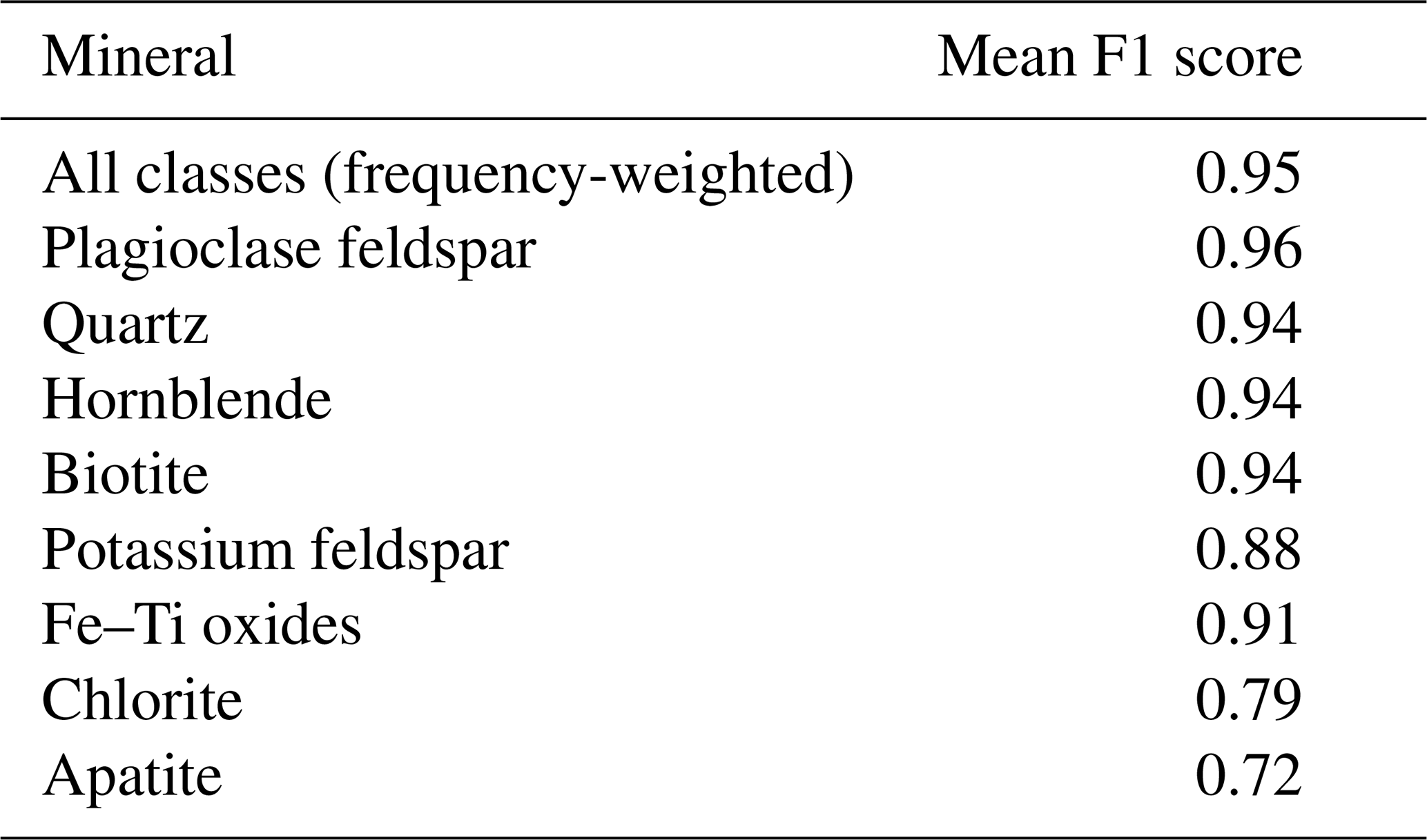
The RF-generated mineral maps in Sect. 3 exhibited high accuracy. For the three thin sections that were mapped both manually and by the RF-based method in Sect. 2, the mean frequency-weighted F1 score among the three thin sections was 0.948±0.002, meaning that nearly 95 % of the pixels in the RF-predicted maps agreed with those in the manually delineated maps (Table 2). The accuracy varied among minerals. The four most abundant minerals (plagioclase, quartz, hornblende, and biotite) all had mean F1 scores of 0.94 to 0.96, while apatite, the least abundant mineral, had the lowest mean F1 score of 0.72. A closer look at the precision and recall metrics for apatite shows that mean recall scores (0.62) were lower than mean precision (0.91). This indicates that the models correctly predicted apatite when attempted but that the models often neglected to predict apatite. Because apatite is rare and appears as small inclusions in our samples, fewer training data were collected for it than for other minerals in each sample. This can result in class imbalances in training data, which, for rare mineral classes (in our case, apatite), can produce scenarios in which the model does not try to predict the mineral class, as the diversity of training data for rare classes (in our case, apatite) remains relatively low (He and Garcia, 2009). Abundance and the mean F1 score were not always linked; for example, Fe–Ti oxides were low in abundance (∼1 %) but registered a mean F1 score of 0.91.

Figure 3 shows an example of an RF-predicted mineral map with misclassified pixels shown in red. This illustrates a key point: the accuracy of the RF-predicted mineral maps is not spatially uniform. Most pixels that diverge from manual classification occur at grain boundaries where elemental compositions shift abruptly in space. By contrast, in mineral grain interiors, divergent pixels are far less common. This indicates that the accuracy of RF-predicted mineralogy in grain interiors is higher than the F1 scores in Table 2.

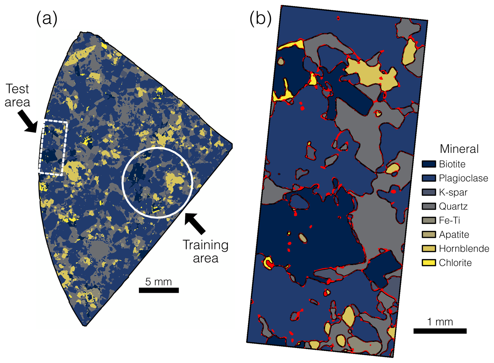
Figure 3 (a) Predicted mineral map for sample 6-3a, showing the location of the manually delineated test map, which we used to check accuracy. (b) Predicted mineral map for the test area. The red areas signify where pixels in the predicted map diverge from the manually delineated test map. This shows that most divergent pixels are at mineral grain boundaries.

A combined confusion matrix for pixel-level comparisons from every test and predicted map showed that the most common divergent classification was chlorite for biotite. This is likely because biotite and chlorite have similar elemental compositions and because they often share a grain boundary (chlorite is a product of hydrothermal alteration of biotite), which means they are more prone to disagreement along grain boundaries. Among the major minerals, our models divergently classified potassium feldspar as plagioclase feldspar most often, likely because many potassium feldspar grains in the Rio Blanco tonalite contain small amounts of Na, such as plagioclase.

Figure 4 shows close agreement between the RF-predicted abundance and the manually mapped abundance in the test areas, with a mean difference for a given mineral of 0.45±0.02 % across the three test maps. So, although some predicted pixels were misaligned spatially, the RF-predicted mineral abundances agree well with manual estimates derived from the test maps.

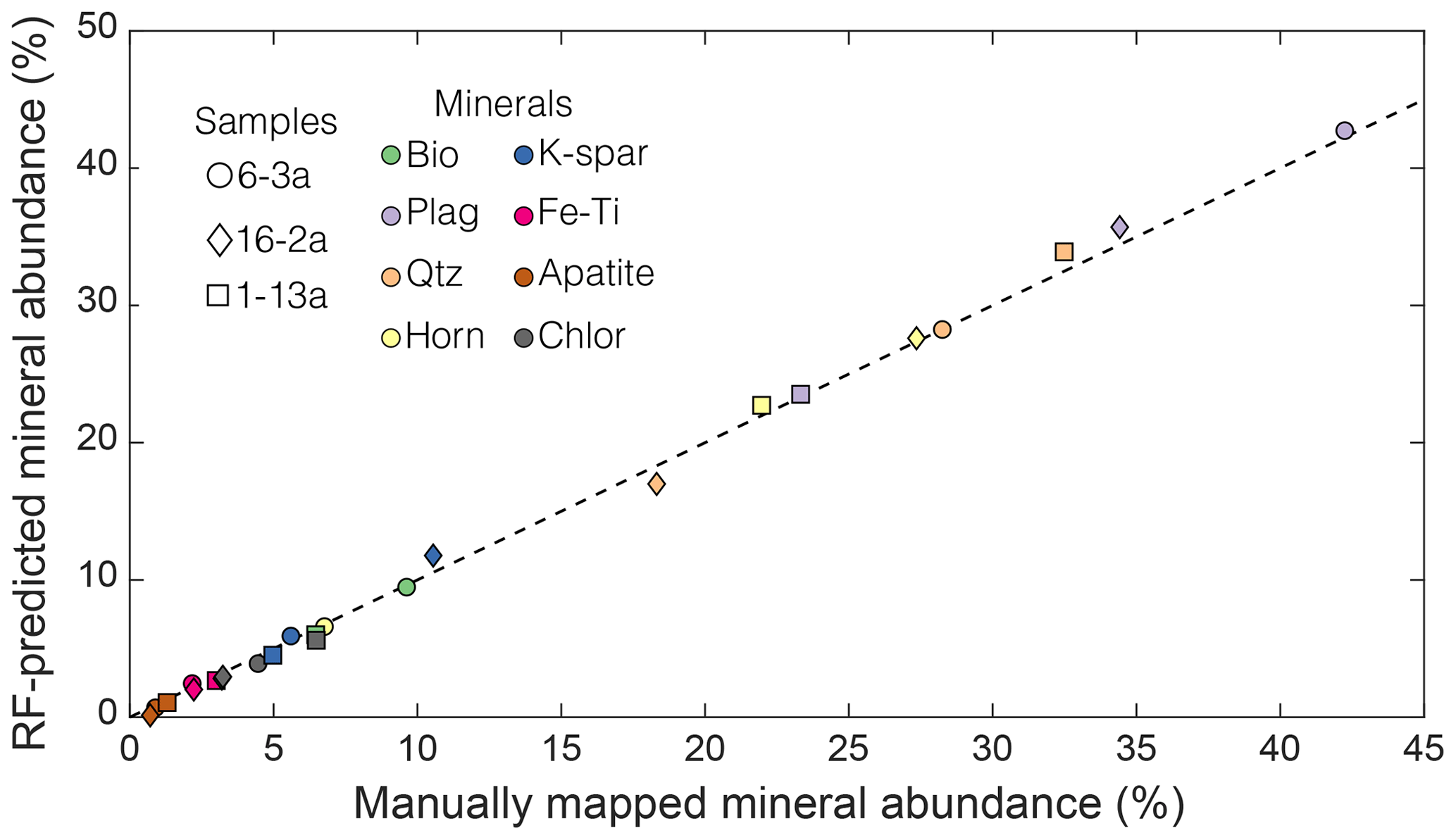
Figure 4 RF-model-predicted mineral abundance vs. manually mapped mineral abundance in the test areas of the three samples with test maps. The dashed line is a 1:1 line. Although there was some spatial mismatch around the edge of mineral grains (e.g., Fig. 3), the RF-predicted modal abundances agree well with abundances inferred from manual mapping in the test areas.

Table 2 Mean F1 scores (accuracy metric) for mineral classes among the three test maps (Fig. 4), based on the comparison of automated mineralogy maps with manually delineated mineralogy maps.

4.2 Sensitivity of mineral maps to random forest hyperparameters and input features

In our application of the method in Sect. 2 to the 14 samples in Sect. 3, we used a set of default values for three RF hyperparameters: maximum tree depth, number of trees, and minimum sample size per node. Reviews of hyperparameter tuning on RF models have shown that the number of trees and the minimum number of classes per node can have a large effect on classification accuracy (Probst et al., 2019). In this section, we gauge the sensitivity of our results to hyperparameter values and input features.

Orfeo ToolBox does not contain a facility for hyperparameter tuning in QGIS, so we developed a workflow to undertake our own hyperparameter optimization outside of QGIS in Python. This is not a necessary step in the method, but we have included this code in the Supplement for users who wish to conduct their own hyperparameter optimization. We began by converting the smoothed elemental intensity image data in the three training areas within the manually delineated test maps into NumPy arrays (Harris et al., 2020) using a combination of three Python libraries: rasterio (Gillies et al., 2019), GeoPandas (Jordahl et al., 2020), and shapely (Gillies et al., 2022). We then used the implementation of the RF classifier from the machine-learning package scikit-learn (Predregosa et al., 2011) for both hyperparameter optimization using a randomized 5-fold cross-validation (Breiman and Spector, 1992) and derivation of feature importance using permutation testing (Breiman, 2001). Through these operations, we seek to find optimal hyperparameters and test the importance of input features (here, elements), respectively.

We used the scikit-learn RandomizedGridCV function to systematically test the sensitivity of the output mineral maps to the RF hyperparameter values. To do this, we trained 100 unique RF models across a range of maximum tree depths (1–100), numbers of trees (10–2000), and minimum sample sizes per node (5–25). These hyperparameters are common between the Orfeo ToolBox and scikit-learn implementations of the RF classifier. We used 5-fold cross-validation, in which each randomly selected set of hyperparameters is used to train the same model five times while sampling different portions of the training data (Breiman and Spector, 1992). We report the best-fit parameters and resultant accuracy in terms of the frequency-weighted F1 score upon comparison to the test maps using these optimized parameters.

Orfeo ToolBox has not yet incorporated a capacity to derive feature importance scores. Feature importance in RF classification is calculated by permutation testing, which is the extent to which an accuracy metric declines if a single input feature's unused training data are randomly altered during the training process and validation process (Breiman, 2001; Guo et al., 2011). We used the scikit-learn function permutation_importance to assess importance using the frequency-weighted F1 score. We report the feature importance for the three samples with manually delineated test maps and discuss their implications.

Tuning the hyperparameters in scikit-learn showed that both a higher maximum tree depth and number of trees may be optimal for our RF models, while the minimum sample for splitting was more variable (Table 3). Using these optimized RF hyperparameters within Orfeo ToolBox yielded a mean frequency-weighted F1 score of 0.95 when comparing the three samples with manually delineated test maps, which is the same F1 score realized by using the default hyperparameters. As the two implementations of the RF classifier are somewhat different in terms of available hyperparameters, the comparison is imperfect but does provide a check to see if the default hyperparameters could be improved upon. That an optimized set of hyperparameters delivered very little to no increase in accuracy is unsurprising, as RF models are known to perform well with little to no tuning if reasonable hyperparameter values are initially used (Maxwell et al., 2018). Unless low F1 scores are realized during Step 4, it is our recommendation that the default RF hyperparameters in Orfeo ToolBox be used.

Table 3 Optimal RF hyperparameters from 5-fold cross-validation performed using scikit-learn.

Feature importance, as determined through permutation testing, showed that both K and Mg were the most important features for our scikit-learn-trained models, with mean decreases in accuracy of 0.29 for both elements based on frequency-weighted F1 scores derived from the training and validation process on unused data (Fig. 5). Ti was relatively unimportant with a very small, slightly positive value, implying it could be omitted. Although Ti is present within biotite and Fe–Ti oxides in our samples, Ti showed little to no decrease in mean accuracy, as both biotite and Fe–Ti oxides can be classified using other elements. We tested whether our feature importance scores were pertinent to models in Orfeo ToolBox by leaving out, in turn, K, Mg, and Ti during the training and validation process. Excluding K decreased mean F1 scores due to the degradation of potassium feldspar, biotite, and chlorite accuracy. In contrast, omitting Mg did not decrease F1 scores, showing that a feature importance score does not directly translate to decreased model accuracy upon omission (Cutler et al., 2011). Leaving out Ti had little effect on F1 scores. If a user of our method is unsure whether an element could be a truly important feature, omitting an important element from the training process by creating virtual rasters without that element should yield a notable degradation in training F1 scores.

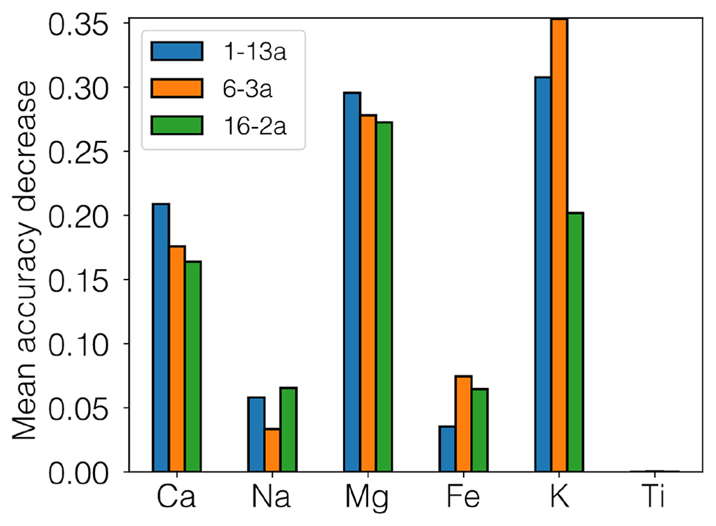
Figure 5 Feature importance from scikit-learn using permutation testing for all six input elements for the three samples with test maps. Mean accuracy decrease is the change in the F1 score due to randomly changing feature data in the unused portion of the training data during the validation process. In Orfeo ToolBox, training models that omitted K degraded F1 scores, while those that omitted Mg yielded little change, indicating that the feature importance score does not always directly map onto model accuracy and that some experimentation with input features (elements) during the training phase is warranted.

4.3 Sensitivity of mineral maps to filter sizes

In our application of this method to our samples, we applied a circular, 7-pixel-radius mean filter to the EDS-generated elemental intensity rasters (Step 2 in Sect. 2), and we applied a circular, 10-pixel-radius majority filter to the output mineral maps (Step 6). To quantify the sensitivity of the output mineral maps to these “hidden” parameters, we generated a series of RF models across a range of mean filter radii for the elemental intensity rasters (no filter and 2, 5, 7, 10, and 20 pixels) and a range of majority filter radii (no filter and 2, 5, 7, 10, and 20 pixels). For the three thin sections with manually delineated mineral maps, we calculated the frequency-weighted F1 score of the entire thin section by comparing each of the RF-predicted mineral maps to the manually delineated test maps.

Figure 6 reveals that both the mean filter and the majority filter affect the accuracy of the predicted mineral maps. The largest impact on the accuracy, as measured by F1 score, was in the application of any mean filter at all to the input elemental intensity rasters. The left panel in Fig. 6 shows that applying no mean filter to the elemental intensity rasters produced low F1 scores (0.52–0.69) for all models and all samples, regardless of the size of the majority filter. Accuracy increased with mean filter radius up to 5 and 7 pixels, which yielded high F1 scores at all majority filter sizes (0.91–0.96) due to the elimination of spurious inclusions within larger mineral grains (middle panels in Fig. 6). Beyond that size, accuracy decreased slightly with higher mean filter radius, with lower F1 scores at radii of 10 pixels (F1 scores of 0.90-0.95) and 20 pixels (0.87–0.89). This implies an intermediate optimal mean filter radius of 5–7 pixels for these samples.

Accuracy was sensitive to the size of the majority filter, particularly for models that applied no mean filter or a small (2-pixel-radius) mean filter to the input elemental intensity rasters (Fig. 6). For the models that applied a mean filter of any size, accuracy was lower at small majority filter radii (0 or 2 pixels) and large radii (20 pixels) than at intermediate majority filter radii (5–10 pixels). At the largest radii, the RF-predicted mineral grains begin to lose shape, becoming more circular. Thus, accuracy was maximized at intermediate majority filter radii of 5–7 pixels, just as it was at intermediate mean filter radii. Excluding plagioclase and quartz (which generally do not occur as isolated grains), the three samples with test maps (6-3a, 1-13a, and 16-2a) have a median grain area of ∼0.005 mm² (n=5188 mineral grains across all three samples), while the 5–7-pixel radii filters have areas of ∼0.001 and ∼0.002 mm², respectively. These optimal sizes most likely result from a mix of the initial EDS pixel resolution and data quality and the types and sizes of minerals in the thin section (Lanari et al., 2014; Ortolano et al., 2018), so we recommend that users experiment to find the optimum filter sizes for their samples.

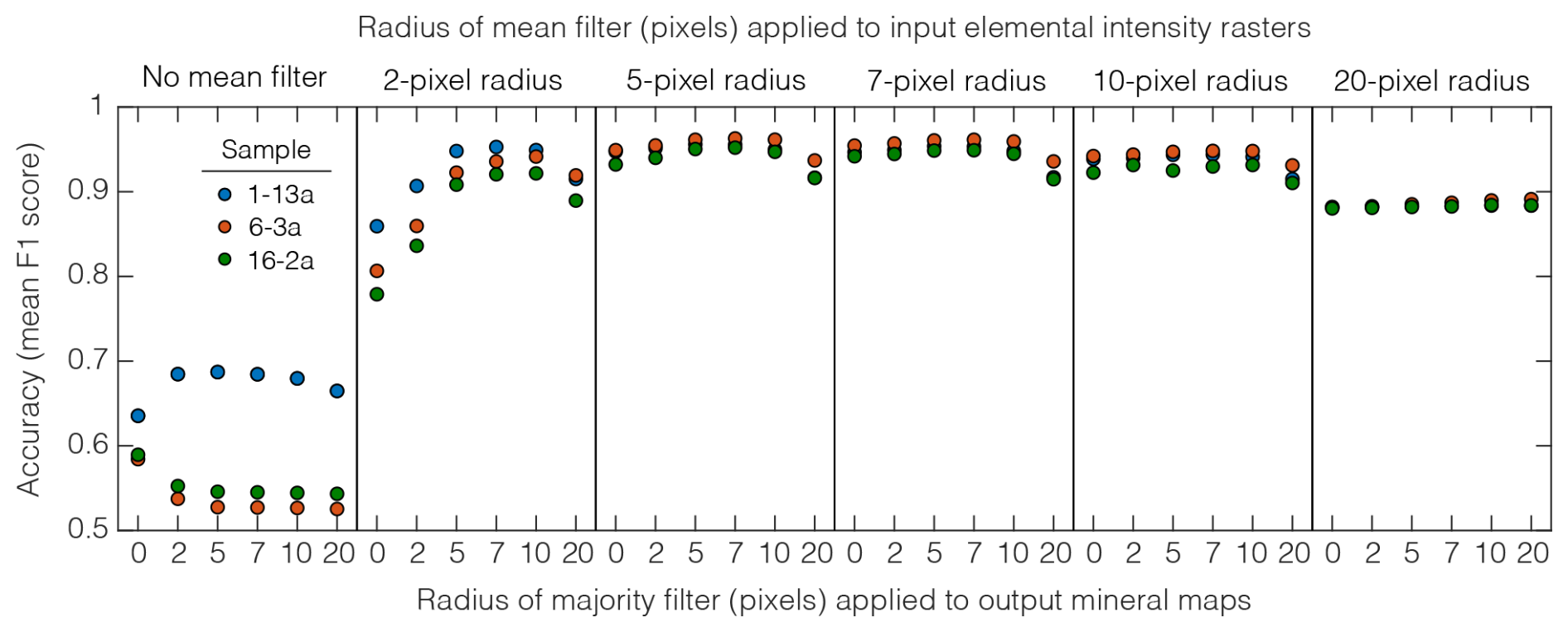
Figure 6 Accuracy of the output mineral maps (as quantified by frequency-weighted mean F1 scores) for combinations of mean filter and majority filter sizes for the three samples with test maps. Each section is a single mean filter size. The most accurate mineral maps (i.e., those with the highest F1 scores) were generated using a 5- or 7-pixel-radius mean filter combined with a 5- or 7-pixel-radius majority filter.

5 Discussion: advantages, utility, and limitations

5.1 Advantages of this open-source automated mineralogy method

Situating our workflow in a free and open-source GIS environment confers several practical benefits. Both Orfeo ToolBox and QGIS are frequently updated with source code that can be examined and modified, unlike many proprietary hardware/software systems (Keulen et al., 2020). Orfeo ToolBox and QGIS each have extensive documentation and user forums monitored by the developers, which can aid in addressing user issues (Raza and Capretz, 2015). Incorporating open-source software into scientific methods fosters transparency and reproducibility as the software is widely accessible and more easily scrutinized (Ramachandran et al., 2021). As both Orfeo ToolBox and QGIS are ongoing efforts with active contributing communities, our no-code workflow is tied to software that is not likely to fall into disrepair or unavailability, unlike much open-source scientific software (Coelho et al., 2020). Furthermore, both Orfeo ToolBox and QGIS are available for all major operating systems, Windows, macOS (Intel), and Linux, so this factor does not limit accessibility. Orfeo ToolBox will likely continue to incorporate new state-of-the-art machine-learning algorithms. For example, Orfeo ToolBox has recently been unofficially extended to utilize the Google TensorFlow library (Abadi et al., 2016) to perform deep-learning tasks on remote sensing imagery (Cresson, 2018, 2022). There are also efforts to develop open-source scanning electron microscope systems and attendant software, such as the NanoMi project (Malac et al., 2022). All of this means that automated mineralogy methods are likely to become more popular and accessible.

We expect that a broad range of geoscientists will be capable of using this GIS-based method, since many geoscience undergraduate programs incorporate GIS into courses (Marra et al., 2017). It requires no programming skill to obtain mineral maps, thereby eliminating a potential barrier for use (Bowlick et al., 2016). Since the workflow takes place within a GIS environment, the input elemental intensity rasters could easily be processed in other ways besides the mean smoothing filter that we applied here, such as edge-detection filtering or elemental intensity ratioing. Creation of optimal input features, so-called feature engineering, is fostered by the many QGIS frontends that interface with SAGA GIS and GDAL raster manipulation programs. Our method does not require a corresponding plugin for Orfeo ToolBox/QGIS, but much of it could be automated from the Orfeo ToolBox/QGIS Python API or as QGIS console commands, if desired. Input parameters for image filters and hyperparameters for the RF models can be saved as JavaScript Object Notation (JSON) files, which can be loaded in later, overcoming some of the reproducibility issues inherent in workflows using graphical user interfaces (Brundson, 2016).

5.2 Illustration of the utility of random forest-generated mineral maps

There are many potential uses for thin-section-scale mineral maps once they have been generated. Converting the mineral maps into vector form allows the calculation of derived parameters, such as the median grain area for minerals that occur as single grains (e.g., biotite), the distance between grains of a mineral, and the types of minerals surrounding a grain or grains in the case of abundant, connected minerals such as plagioclase and quartz. These types of data are normally generated by proprietary automated mineralogy systems but could aid in geoscience disciplines beyond ore geology or petroleum geology (Han et al., 2022). An illustrative example is in the analysis of grain-scale properties of biotite. This is of wide interest because the oxidation of ferrous Fe in biotite drives the expansion of biotite grains, which generates stresses in the surrounding rock that may be large enough to fracture the rock (Fletcher et al., 2006; Goodfellow et al., 2016; Goodfellow and Hilley, 2022). To the extent that biotite expansion promotes the generation of regolith from bedrock, it may even influence the kilometer-scale evolution of mountainous topography (Wahrhaftig, 1965; Xu et al., 2022). In granitic rocks, numerical modeling has shown that biotite abundance influences the accrual of microscale damage (Shen et al., 2019) and that weathering profile development is partially guided by biotite crystal size (Goodfellow and Hilley, 2022). These are two properties that can be directly measured in our thin-section-scale mineral maps.

To obtain such mineral maps in some previous studies, researchers have often engaged in manual or semi-automated characterizations of sample mineral properties (Buss et al., 2008; Ündül, 2016). These workflows are often tailored for a single study (e.g., Goodfellow et al., 2016). Methods that are based on generalizable workflows involving automated mineralogy methods, such as the one presented in this study, could enhance comparability between studies. Since we converted the predicted mineral maps into a vector (polygon) form within QGIS, we could use built-in functions to gather large amounts of data on grain neighbors or perform grain size measurements. As we discuss in Sect. 5.3, classified biotite “grains” may contain multiple bordering crystals of the same mineral as our EDS input data, and the resultant classification cannot differentiate boundaries by elements alone (Lanari et al., 2014). As biotites are relatively isolated from each other in our thin sections, these measurements serve as a reasonable indicator of true biotite properties. For example, the 20 largest biotite grains in samples 1-1a and 6-3b comprise 80 % and 94 % of the total biotite area, respectively (Fig. 7a–b). The median grain area of these 20 biotite grains in sample 1-1a is 0.60 mm², several times larger than that in sample 6-3b (0.19 mm²; Fig. 7c).

We can also use raster morphology operations on the mineral maps to measure distances between classified minerals. In analog and numerical experiments that impose stress on granitic rocks (Tapponier and Brace, 1976; Li et al., 2003; Mahboudi et al., 2012), biotite grains can act as preferential origination points for microfractures, but biotite can also arrest propagation of microfractures arising from neighboring grains. Thus, the distance between biotite grains may be an important, yet rarely measured, property. In the example of the two samples in Fig. 7, biotite grains have similar median distances from one another but different probability distributions of distances between biotite grains, particularly in the long tail of the distributions at larger distances (Fig. 7e). We can also extract the composition of neighboring grains surrounding biotite (Fig. 7f), which reveal that chlorite is much more abundant near biotite relative to the rest of the thin section. Data like these can be useful for those studying the impacts of different grain–grain contacts on stress response during rock mechanics experiments (e.g., Aligholi et al., 2019), which have shown that some mineral interactions can have an outsized influence on the development of fractures and failure. In sum, the data in Fig. 7 illustrate the potential power of RF-generated mineral maps to improve quantitative in situ investigations of biotite weathering (Behrens et al., 2021) and form the basis for more realistic models of biotite-driven rock damage (Shen et al., 2019).

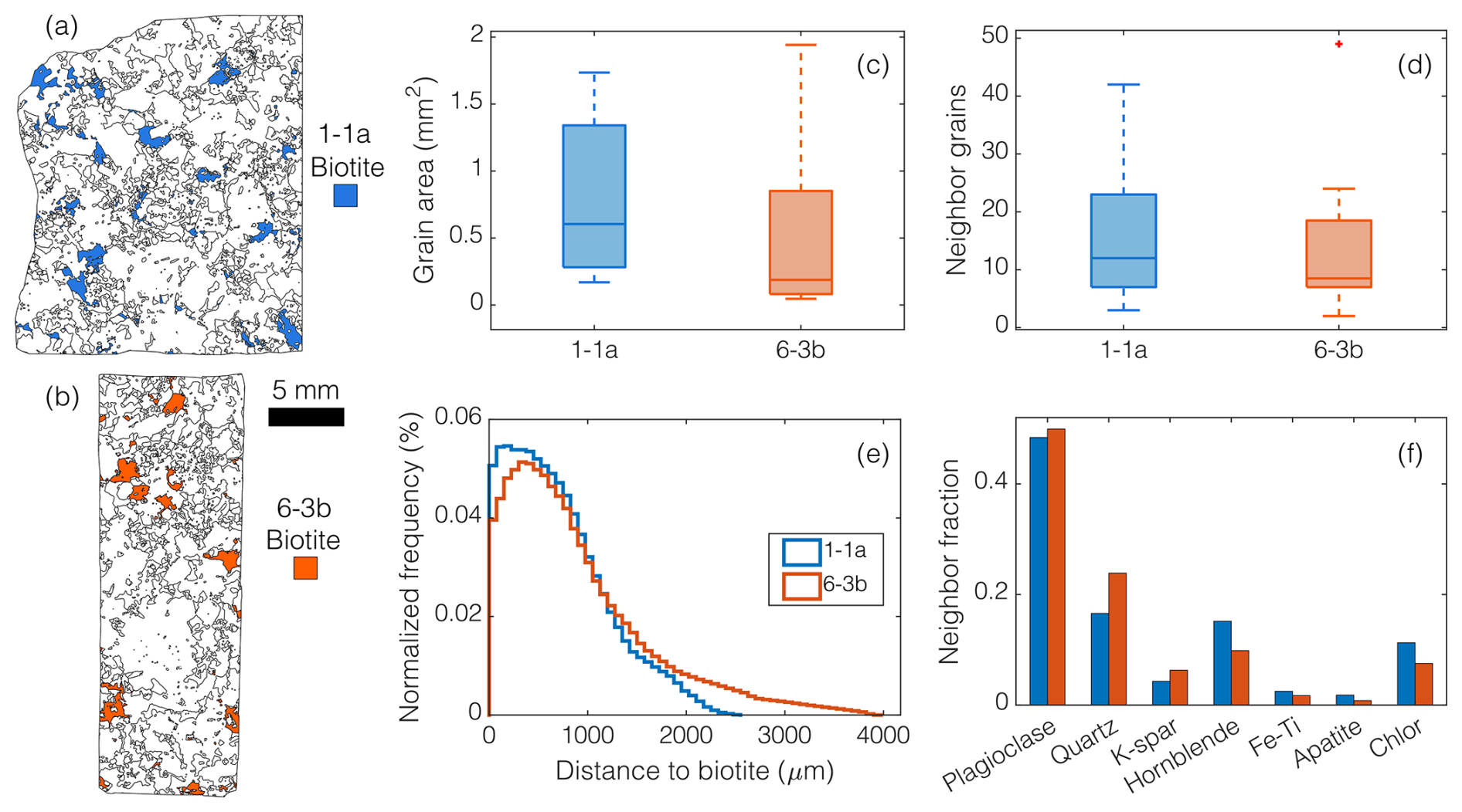
Figure 7 Example of quantities that can be obtained from mineral maps generated by the automated method in this study. (a–b) Colors highlight biotite grains identified in the RF-generated mineral maps in thin sections 1-1a (blue) and 6-3b (orange). (c–f) Biotite properties extracted from predicted maps for the 20 largest biotite grains in each sample. These data could help inform numerical models of microcrack generation and allow quantitative comparisons between different samples or lithologies (e.g., Shen et al., 2019). (c) Boxplot of biotite grain area (mm²) for the 20 largest biotite grains for both samples. (d) Boxplot of number of grains surrounding the 20 largest biotite grains. (e) Normalized frequency distribution of distances between biotite pixels (not including those inside a biotite grain). (f) Composition of neighbors as a fraction of perimeter.

5.3 Limitations

Our method's greatest asset is that it can generate thin-section-scale mineral maps without requiring the use of propriety software or a background in programming. Its most important limitation is that it is most accurate if the user trains an RF model for every thin-section sample. Using an RF model that was trained on one sample to predict mineral maps for another sample can yield mineral maps that accurately map minerals in some areas but inaccurately map them in others. For example, when we applied an RF model that was trained on sample 16-2a to sample 6-3a, apatite abundance was overpredicted by a factor of 5, possibly due to 6-3a having some highly calcic zones within plagioclase grains. So, for the most accurate results, we recommend training each thin section separately.

A second limitation is that this method tends to be less accurate at identifying low-abundance minerals. Unlike some proprietary automated mineralogy software systems, our method does not use predefined EDS spectra to identify minerals. Instead, our method trains RF models on the samples themselves, which means that each mineral of interest must be abundant enough to properly train the RF model. The relatively low F1 scores of the lower-abundance minerals in our samples (Table 2) suggest that the minimum abundance required to train an RF model is larger for minerals with small grain size (e.g., in the case of apatite) and a lack of compositional distinction (e.g., in the case of chlorite). Minerals must be resolvable by the EDS data, so collecting EDS data with a field-emission-gun SEM at higher resolution (∼0.1 µm) could improve mineral classification in rocks with finer grain size distributions (Han et al., 2022).

A final limitation is that mineral grains that border mineral grains of the same mineral appear to the RF model as regions of the same mineral and hence can be classified as a single mineral grain, rather than two grains. This is a common issue shared with other automated mineralogy methods (Lanari et al., 2014; Hrtska et al., 2019), and it can affect inferred probability distributions of mineral grain size of those minerals if not properly accounted for.

6 Conclusions

The main contribution of this study is a new automated method for obtaining mineral maps from EDS scans of rock thin sections. This method is implemented within a free and open-source GIS application, uses free and open-source plugins for RF image classification, and requires no programming. To demonstrate the utility of this method, we trained RF models on EDS scans of 14 thin-section samples of a well-studied plutonic igneous rock. The resulting model-predicted mineral maps compare well with manually delineated mineralogy maps, with 95 % of pixels on the mineral maps predicted correctly. With regard to the most abundant minerals in the Rio Blanco tonalite, plagioclase feldspar and quartz, the models attained 96 % and 94 % accuracy, respectively.

We utilized scikit-learn's implementation of the RF classifier to search for optimal RF hyperparameters and to test input feature (element) importance. We saw no increase in accuracy using optimal hyperparameters found in scikit-learn when used within Orfeo ToolBox, so we recommend using the default hyperparameters. We did see that an important input feature, K, did lower accuracy when not included in Orfeo ToolBox-based models, so some level of experimentation with input features during the training step is warranted. We also tested to see if our pre- and post-processing steps had a large influence on accuracy by using different sizes of mean and majority filters. An absence of filtering and excessively large filters led to lower accuracy, while filters in the range of 5–10 pixels for both mean and majority filters led to higher accuracy.

Situating the workflow within a free and open-source GIS environment confers distinct advantages. Open-source environments extend benefits such as source code availability, extensive documentation, and accessibility. Moreover, as the workflow is within a GIS environment, the application is likely to be familiar to a range of geoscientists. Also, all the available tools (e.g., different types of image filters) within the GIS allow easy input feature experimentation. The mineral maps from our method proved highly accurate when compared to manually delineated maps, and estimates of mineral abundance compared well to previous estimates from the literature for our sample lithology. Many of the measured quantities produced by proprietary automated mineralogy systems are obtainable once predicted mineral maps are converted to vector datasets. These measurements, such as median grain size and amount of grain neighbors, can be useful to researchers studying microscale damage processes that arise through rock weathering or rock mechanics experiments. We hope that this method will be useful for researchers who wish to obtain rapid, automated mineralogy maps of thin sections.