Ice borehole thermometry: sensor placement using greedy optimal sampling

Borehole thermometry is an important tool for reconstructing past climate conditions, assessing changes in land energy storage, and understanding subsurface thermal regimes such as permafrost and glacial dynamics. Optimizing the temperature sensor placement within boreholes allows us to maximize the informativeness of temperature measurements, particularly in polar regions where operational constraints necessitate cost-effective solutions. Traditional sensor placement methods such as linear or exponential spacing, often overlook site-specific subsurface ice heat distribution characteristics, potentially limiting the accuracy of the measured temperature profile. In this paper, we propose a greedy optimal sampling technique for strategically placing temperature sensors in ice boreholes. Utilizing heat transfer model simulations, this method selects sensor locations that minimize interpolation errors in reconstructed temperature profiles. We apply our approach to two distinct ice borehole sites: EPICA Dronning Maud Land site in East Antarctica and the Greenland Ice Core Project site, each with unique surface conditions. Our results demonstrate that the greedy optimal sensor placement significantly outperforms conventional linear and exponential spacing methods, reducing sampling errors by up to a factor of ten and thus achieving similar informativeness with fewer sensors. This strategy offers a cost–effective means to maximize the information obtained from ice borehole temperature measurements, thereby potentially enhancing the precision of climate reconstructions.

1 Introduction

The Earth's climate system is experiencing an imbalance, with continuous accumulation of heat over the past decades, leading to warming across various components including the ocean, land, cryosphere, and atmosphere (von Schuckmann et al., 2023). High precision measurements of subsurface ice and soil temperatures are essential for assessing changes in land energy storage, refining ice models (Løkkegaard et al., 2023), and determining the thermal state of permafrost (Biskaborn et al., 2019; Eppelbaum, 2024). Subsurface temperature profiles obtained through borehole thermometry provide valuable information about the surface temperature evolution, glacial thermal regimes, and geothermal heat flux (Orsi et al., 2012; Cuffey et al., 2016; Montelli and Kingslake, 2023; Groenke et al., 2024). Borehole temperature logs used for climate reconstruction must balance the precision of temperature measurements with the depth resolution (Beltrami, 2002). In addition, temporal resolution plays an important role: while many borehole temperature measurements are performed at a single point in time by continuously or stepwise lowering a single sensor, continuous measurements over time have several advantages. These continuous measurements help average out seasonal effects or fast temporal fluctuations, utilize transient data to better constrain the inverse temperature reconstruction problem (Clow, 1992), and allow for measurements in boreholes that are still disturbed from the drilling process. For example, Muto (2010) placed a temperature chain with 16 temperature sensors in 80–90 m deep boreholes. Continuous measurements were then performed for over a year and sent via satellite with the objective of reconstructing multi-decadal temperature trends in East Antarctica. This strategy allowed the team to discard the initial months when the borehole was still affected by the drilling process and to average out the seasonal cycle, all without requiring a second expedition to return to the borehole. Thus, high precision temperature measurement technology for continuously monitoring borehole temperatures is an important tool for climate reconstructions. The system's ability to withstand extremely cold temperatures, its ultra low power consumption, and its high precision and long-term stability are crucial (Løkkegaard et al., 2023). To minimize costs and allow this temperature sensing and data transmission system to operate over multiple years on limited energy supplies, it may be necessary to compromise on the number of sensing devices. Therefore, one needs to be strategic about where to place the limited number of sensors in the borehole to maximize the informativeness of the measurements with minimal effort.

The distribution of heat in boreholes is mostly determined by diffusion and advection of surface temperature anomalies as well as the geothermal heat flux (Cuffey and Paterson, 2010). Temperature logs from terrestrial boreholes used to reconstruct surface temperature histories vary widely in the number of measurements, ranging from 10 to over a hundred for 200–600 m deep borehole profiles (Pollack et al., 1998). For surface temperature reconstruction, Muto (2010) and Zagorodnov et al. (2012) used an ad hoc spacing of temperature sensors in the borehole, with the distance between the sensors increasing down the borehole. Clow (1992) suggested that by exponential positioning of sensors, each data point contributes an identical amount of information to a reconstructed surface temperature history. Beyond sensor placement, uncertainties in borehole-based reconstructions can also arise from factors such as insufficient borehole depth, which hinders the separation of climatic and geothermal signals (Beltrami et al., 2015), and heterogeneous thermal properties of soils and bedrock, which vary with depth and location (Shen et al., 1995; García-Pereira et al., 2024). These challenges are typically less significant in ice boreholes, where the thermal properties of snow and ice are homogeneous and well known and the boundary conditions are generally better constrained. Although the topic holds significance and potential, sensor placement in boreholes has not received much attention in the field of ice borehole thermometry.

At the same time, the sensor placement problem has been extensively studied in other research areas such as weather forecasting and environmental monitoring. A study conducted to control the environment inside the greenhouse, used error based and entropy based methods for optimal sensor placement to track temperature variations (Lee et al., 2019). Active data selection and test point rejection based on error variance (Seo et al., 2000), Gaussian Process based model to reduce uncertainty (Singh et al., 2006; Krause et al., 2008), and convolutional Gaussian neural process (Andersson et al., 2023) are few of the machine learning related approaches for sensor placement. Finding effective sensor placements in the context of borehole thermometry can be accomplished by applying similar ideas of selecting sensor positions to minimize error.

The knowledge of the heat distribution in ice is necessary for determining the best location of sensors for ice borehole thermometry. Snow falls on top of the ice sheet and is then densified into firn, eventually becoming ice at a depth of approximately 80–100 m. Over time, heat gradually diffuses into the ice, with stronger fluctuations in temperature occurring closer to the surface and smoothing out deeper within the ice sheet. This phenomenon primarily motivates the ad hoc placement of borehole sensors discussed above, where the distance between measurement points increases further down the borehole (Clow, 1992; Muto, 2010; Zagorodnov et al., 2012).

In this paper, we propose an approach to strategically install a set of sensors to measure the temperature of an ice borehole to gather information on borehole temperature profile as effectively as possible. Using heat transfer model simulations, a greedy sampling technique is employed to optimize the sensor placement. Greedy algorithms solve problems by selecting the solution that is locally optimal at each phase (Black, 2005). We start by formularizing a greedy optimal sampling algorithm for finding sensor placements in the borehole. We evaluate the approach of greedy optimal sensor placement for two distinct boreholes with distinct local surface conditions and examine our findings by contrasting it with the linear and exponential sensor placements. To demonstrate how to find an optimal and cost-effective arrangement of sensors, we analyze how the informativeness of borehole thermometry depends on the number of sensors used. We further discuss the uncertainty in the algorithm and data used in this study.

2 Method and data

We discuss the underlying subsurface ice heat transfer model, which is given as a one-dimensional diffusion advection equation. The sensor placement problem is solved by using a greedy optimal sampling algorithm that utilizes the heat transfer model applied to a set of possible past surface temperature evolutions to include the physics of the problem into the sensor optimization. We also describe the physical parameters of the two example sites considered in this study.

2.1 Heat transfer model

The heat transfer of the surface temperature θ(t) into the ice sheet is modeled by the one-dimensional heat diffusion advection equation

$$\begin{array}{}\text{(1)}& {\displaystyle \frac{\partial T_{\mathit{\theta }}}{\partial t}}=k{\displaystyle \frac{{\partial }^{\mathrm{2}}{T}_{\mathit{\theta }}}{\partial z^{\mathrm{2}}}}-w{\displaystyle \frac{\partial T_{\mathit{\theta }}}{\partial z}},\end{array}$$

where T_θ is the temperature as a function of time t and depth z (positive downwards). As a convention, the model is defined for time $t\in [t_{\mathrm{0}},t_{\mathrm{pr}}]$, hence heat transfer is considered from t₀ years in the past to the present time (t_pr). w is the vertical velocity and k is the thermal diffusivity. The thermal diffusivity is calculated as

$$\begin{array}{}\text{(2)}& k={\displaystyle \frac{K}{\mathit{\rho }c}},\end{array}$$

where c is the specific heat capacity, K is the thermal conductivity, and ρ is the density of the firn/ice. Details of the parametrization of density, thermal properties and vertical velocity are given in Appendix A. The (vertical) spatial domain is [0,H], where H is the thickness of the ice sheet and z=0 corresponds to the surface, see Fig. 1. Note that we consider [0,L] (L<H) as the subdomain of the borehole in ice, while still modeling the full vertical temperature profile on domain [0,H], which includes the borehole and the below remaining ice sheet.

To solve Eq. (1), we use the forward Euler method in time, central differences for the diffusion term, and forward differences for the advection term. The spatial grid (in z direction) with uniform step size Δz is ${\mathit{Z}}_{\mathrm{F}}\subset [\mathrm{0},H]$. We employ Dirichlet boundary conditions for the simulations in this study. The boundary conditions are given as

$$\begin{array}{}\text{(3a)}& {\displaystyle }{T}_{\mathit{\theta }}(t,\mathrm{0})=\mathit{\theta }\left(t\right),\text{(3b)}& {\displaystyle }{T}_{\mathit{\theta }}(t,H)={\mathit{\theta }}_{\mathrm{b}},\end{array}$$

representing the top and bottom boundary conditions of the model. The top boundary condition models the input of the surface temperature into the ice sheet. The bottom boundary condition is set to the basal temperature of the ice sheet θ_b. In order to determine the initial condition (T_θ(t₀,z)), the model is run for 50 000 years by setting the top boundary condition to a constant mean temperature $T_{\mathit{\theta }}(t,\mathrm{0})={\mathit{\theta }}_{\mathrm{m}}$, until the profile reaches equilibrium. The result of the temperature profile simulation for surface temperature θ(t) is T_θ(t_pr,z) which can be denoted as T_F. This represents the vector of approximated temperatures at all grid points Z_F of the discretized heat transfer model.

2.2 Sensor placement problem

Our goal is to select the set of n best sensor locations Z_S in the borehole of depth L (Fig. 1), so that the sampling error in the reconstruction of the borehole temperature profile is minimized. The sensor locations Z_S are selected from a set of candidate sensor locations Z_L. Here, this set is selected as a uniform grid of size l, over the interval [0,L], where l is the number of possible candidate sensor locations.

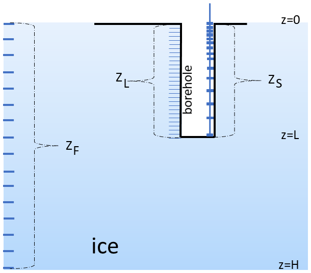
Figure 1 Schematic diagram representing space vectors used in the algorithm. Z_S is the set of selected sensor locations, Z_L is the grid of candidate sensor locations, and Z_F is the spatial grid of the model.

2.2.1 Sampling error calculation

Our aim is to develop a measure of error or uncertainty, for a given choice of sensor placements Z_S. To this end, we evaluate simulated temperature profiles for different surface temperature evolutions at locations Z_S to find the respective set of temperature values T_S. Then, we estimate the (interpolation) error that we introduce if we aim to recover the full temperature profiles from this artificial data (Z_S and T_S for each profile). We use cubic spline interpolation for this study (Fig. C1 in Appendix C). Sampling error is calculated as the root mean square over these interpolation errors obtained for each of the given temperature profiles of possible surface temperature histories, thereby incorporating a prior assumption on possible past surface temperature evolutions. This procedure is formulated in Algorithm 1.

Note that in our algorithm, the final sampling error (ϵ_s) is influenced by the error due to sensor placement (i.e., interpolation error) and by the error due to uncertainties in the sensor device, which is called device error (ϵ_d). Here, ϵ_d is drawn from a normal distribution $\mathcal{N}(\mathrm{0},{\mathit{\sigma }}_{\mathrm{d}}^{\mathrm{2}})$ and is considered independent between borehole simulations and across sensors. The artificial temperature measurements T_S for sensors Z_S are generated by adding an error term ϵ_d.

Algorithm 1 Sampling_error.

Input: Sensor locations Z_S, standard deviation of sensor device error σ_d, a set of P temperature profiles $\mathit{\{}{\mathit{T}}_{{\mathrm{F}}_p}{\mathit{\}}}_{p=\mathrm{1}}^P$, candidate sensor locations Z_L.

Output: Sampling error ϵ_s

begin:

p←1

while p≤P do

Create an interpolating function ${\stackrel{\mathrm{̃}}{T}}_{\mathrm{F},p}$ for the pth simulated temperature profile, ${\stackrel{\mathrm{̃}}{T}}_{F,p}\left(z\right)\leftarrow \mathbb{I}({\mathit{Z}}_{\mathrm{F}},{\mathit{T}}_{{\mathrm{F}}_p})$.

Draw device error ϵ_d from normal distribution with given standard deviation $\mathcal{N}(\mathbf{0},{\mathit{\sigma }}_{\mathrm{d}}^{\mathrm{2}}\mathbf{I})$.

Create artificial measurements ${\mathit{T}}_{{\mathrm{S}}_p}$ for sensors in Z_S using the function ${\stackrel{\mathrm{̃}}{T}}_{\mathrm{F},p}$ and device error, ${\mathit{T}}_{{\mathrm{S}}_p}\leftarrow {\stackrel{\mathrm{̃}}{T}}_{\mathrm{F},p}\left({\mathit{Z}}_{\mathrm{S}}\right)+{\mathit{ϵ}}_{\mathrm{d}}$.

Create interpolation function ${\stackrel{\mathrm{̃}}{T}}_{\mathrm{S},p}$ for sensor locations and artificial sensor measurements, ${\stackrel{\mathrm{̃}}{T}}_{\mathrm{S},p}\left(z\right)\leftarrow \mathbb{I}({\mathit{Z}}_{\mathrm{S}},{\mathit{T}}_{{\mathrm{S}}_p})$.

Calculate error grid as the difference between two functions evaluated at all candidate locations, ${\mathit{ϵ}}_{{\mathrm{s}}_p}=\left[\right|{\stackrel{\mathrm{̃}}{T}}_{\mathrm{S},p}\left(z\right)-{\stackrel{\mathrm{̃}}{T}}_{\mathrm{F},p}\left(z\right)|{]}_{z\in {\mathit{Z}}_{\mathrm{L}}}$.

$p\leftarrow p+\mathrm{1}$

end while

Calculate final sampling error as the root mean square across error grids with respect to all P profiles, ${\mathit{ϵ}}_{\mathrm{s}}=\sqrt{\frac{{\sum }_{p=\mathrm{1}}^P({\mathit{ϵ}}_{{\mathrm{s}}_p}{)}^{\mathrm{2}}}{P}}$.

end

Algorithm 1 thus requires the given choice of sensor locations, standard deviation of sensor device error, a set of borehole temperature profiles, and all possible (candidate) sensor locations for the calculation of sampling error. For each of the borehole temperature profiles, the algorithm creates an interpolation function. Artificial sensor measurements are created by evaluating given sensor locations using this interpolation function and adding device error to them. A separate interpolation function is then created for this artificial measurements. Both these functions are evaluated at all possible candidate locations, and the difference between them is recorded as the error grid for each borehole temperature profile. The final sampling error is calculated as the root mean square of the error grids of all borehole temperature profiles.

2.2.2 Sensor placement using greedy optimal sampling

Greedy optimal sampling is an adaptive method of adding sensors to lower the sampling error (Krause et al., 2008; Bartos and Kerkez, 2021). The sampling error is computed after each sensor is added, and the subsequent sensor is positioned at the location on the grid of candidate sensor locations Z_L, which has the maximum error.

This procedure is summarized in Algorithm 2. The algorithm begins by initializing Z_S with a set of sensor positions ${\mathit{Z}}_{\mathrm{S}}^{*}$, in which one sensor is fixed to the top and one to the bottom position of the borehole, while the others are randomly selected using a quasi-random sequence with upper bound as L and lower bound as 0. The sampling error ϵ_s which represents the accumulated error over all candidate sensor location Z_L (refer Sect. 2.2.1) is calculated with respect to the current set of sensor positions in Z_S. The algorithm identifies the next sensor position z_opt as the location in Z_L which has the maximum error. The optimal sensor position z_opt thus found from the set of candidate sensor locations is added to the existing set of selected sensor positions in Z_S, and this process is repeated with updated Z_S each time, until all the remaining sensor positions are found.

There is a possibility of bias in the sensor locations Z_S found using Algorithm 2 resulting from ${\mathit{Z}}_{\mathrm{S}}^{*}$ being fixed at the beginning. This is reduced by averaging the various sets of sensor locations Z_S obtained with respect to different ${\mathit{Z}}_{\mathrm{S}}^{*}$ in the greedy optimal sampling algorithm (Algorithm 2). We average these different sets of Z_S giving averaged sensor placements $\stackrel{\mathrm{‾}}{{\mathit{Z}}_{\mathrm{S}}}$. It is assumed that this averaging procedure allows to reduce the bias due to ${\mathit{Z}}_{\mathrm{S}}^{*}$ being fixed (also see Sect. 4.1). $\stackrel{\mathrm{‾}}{{\mathit{Z}}_{\mathrm{S}}}$ is referred to the greedy optimal sensor placement in this study, and unless otherwise specified, $\stackrel{\mathrm{‾}}{{\mathit{Z}}_{\mathrm{S}}}$ is obtained by averaging over 1000 sets of Z_S.

Algorithm 2 Greedy optimal sampling.

Input: No. of available sensors n, initial set of sensor locations ${\mathit{Z}}_{\mathrm{S}}^{*}$, standard deviation of sensor device error σ_d, a set of P temperature profiles $\mathit{\{}{\mathit{T}}_{{\mathrm{F}}_p}{\mathit{\}}}_{p=\mathrm{1}}^P$, candidate sensor locations Z_L.

Output: Set of sensor locations Z_S

begin:

Initialize the set of sensor locations, ${\mathit{Z}}_{\mathrm{S}}\leftarrow {\mathit{Z}}_{\mathrm{S}}^{*}$.

Set n^* with the size of initial set of sensor locations ${\mathit{Z}}_{\mathrm{S}}^{*}$.

$i\leftarrow n^{*}$

while $i<(n-n^{*})$ do

Find the sampling error ϵ_s for the current set of sensor locations, ${\mathit{ϵ}}_{\mathrm{s}}\leftarrow \text{sampling\_error}({\mathit{Z}}_{\mathrm{S}},{\mathit{\sigma }}_d,{\mathit{Z}}_{\mathrm{F}},\mathit{\{}{\mathit{T}}_{{\mathrm{F}}_p}{\mathit{\}}}_{p=\mathrm{1}}^P,{\mathit{Z}}_{\mathrm{L}})$.

Select the location from Z_L that corresponds to maximum error in ϵ_s as the next sensor location in-order to minimize sampling error,

$\widehat{j}\leftarrow \arg {max}_j{\mathit{ϵ}}_{\mathrm{s}}^{\left(j\right)}$,

$z_{\text{opt}}\leftarrow Z_{\mathrm{L}}^{\left(\widehat{j}\right)}$.

Add z_opt to the current set of sensor locations, ${\mathit{Z}}_{\mathrm{S}}\leftarrow {\mathit{Z}}_{\mathrm{S}}\cup z_{\mathrm{opt}}$.

Sort the set Z_S.

$i\leftarrow i+\mathrm{1}$

end while

end

2.2.3 Other sensor placement schemes

Linear and exponential spacing of sensor locations are used for comparative analysis in this paper. In what we denominate as linear sensor placement, sensors positions z_i∈Z_S are assumed to be equally spaced along the sample space, hence

$$z_i=\left\{\begin{array}{lr}(i-\mathrm{1})d& \mathrm{1}\le i<n\\ L& i=n\end{array}\right.$$

where, $d=\frac{L}{n-\mathrm{1}}$. In exponential sensor placement, sensors positions z_i∈Z_S are assumed to be spaced evenly on a log scale along the sample space, hence

$$z_i=\left\{\begin{array}{lr}(r{)}^{i-\mathrm{1}}-\mathrm{1}& \mathrm{1}\le i<n\\ L& i=n\end{array}\right.$$

where, r is the common ratio between adjacent sensor positions.

2.3 Data

2.3.1 Parameters of the study sites

We study two known ice coring sites chosen to represent distinct boundary conditions (Table 1): EPICA Dronning Maud Land drilling site at Kohnen Station, East Antarctica (EDML) (75.00° S, 0.07° E) (Wesche et al., 2016), and the site of the Greenland Ice Core Project (GRIP) (72.35° N, 38.30° W). GRIP has an accumulation rate of 230 mm yr⁻¹ (Hammer and Dahl-Jensen, 1999) and a mean surface snow temperature of −31.7 °C (borehole temperature at 10 m) (Johnsen, 2003), while EDML has a lower accumulation rate of 64 mm yr⁻¹ (Oerter et al., 2004) and a mean surface snow temperature of −44.1 °C (borehole temperature at 10 m, measured in 2024).

Table 1 Basic parameters of the heat transfer model.

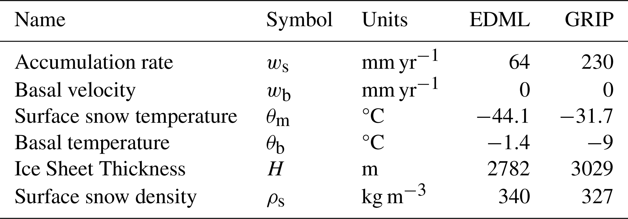
Accumulation rates: GRIP (Hammer and Dahl-Jensen, 1999) and EDML (Oerter et al., 2000, 2004), Snow surface temperature: GRIP (Johnsen, 2003) and own measurements 2024, Basal temperature and ice sheet thickness: GRIP (Thorsteinsson et al., 1997) and EDML (Weikusat et al., 2017), Surface pressure: (Hersbach et al., 2020), Snow surface density: GRIP (Bolzan and Strobel, 1994) and EDML (Ligtenberg et al., 2011).

The heat transfer model is discretized with a temporal grid of size 15 984 ($\mathrm{\Delta }t={\mathrm{2}}^{-\mathrm{4}}$ years) and the spatial grid of size 695 for EDML and 757 for GRIP leading to a spatial resolution of Δz∼4 m for both sites.

2.3.2 Surface temperature time series

We generate an ensemble of surrogate local surface temperature time series designed to capture the full range of possible temperature histories. Each surrogate is a random time-series (η(t,β)) following a power law spectral density with β as its scaling exponent and the variance of the local observed surface temperature, as well as a global warming component based on anomalies in global mean temperatures (GMT) multiplied by a factor PA, representing the potential amount of polar amplification at the borehole site.

$$\begin{array}{}\text{(4)}& \mathit{\theta }\left(t\right)=\mathit{\eta }(t,\mathit{\beta })+\mathrm{PA}\times \mathrm{GMT}\left(t\right)\end{array}$$

In particular, this approach considers the temporal covariance structure of the stochastic component, which mimics natural climate variability (such as weather), and accounts for the uncertain amplitude of the deterministic warming trend. A simple parametrization to describe observed climate variability across a wide range of timescales is to assume a power–law relationship for the power spectral density (PSD) of the signal, S(f) (Laepple and Huybers, 2014). This relationship is expressed as

$$\begin{array}{}\text{(5)}& S\left(f\right)\propto f^{-\mathit{\beta }},\end{array}$$

where β represents the scaling exponent. In state-of-the-art climate models, a scaling exponent of β=0.2 is typically found for Antarctica (Casado et al., 2020). However, data from the EDML ice core and nearby ice cores for the past 1000 years suggest a scaling exponent of approximately β=0.6 after adjusting for local non-climate variability (Münch and Laepple, 2018). In contrast, marine and terrestrial temperature proxy data indicates a scaling exponent closer to β=1 (Hébert et al., 2022). In this study, we select values of β between 0 and 1 to encompass the range of plausible scaling behaviors for surface temperature.

We generate 1000 year long surrogate time series as the sum of a realization of a stochastic process mimicking natural variability and the global mean surface temperature time series to represent the global warming component. The random time series follow the prescribed power-law spectral density and have the variance of the observed 2 m air temperature time-series from the ice core locations from NOAA 20th century reanalysis (Compo et al., 2015) spanning 1836–2015. The global warming component are the anomalies in the NOAA 20th century reanalysis global mean temperature (GMT) with respect to mean value in 1836–1950 and multiplied by factor $\mathrm{PA}=\mathrm{1},\mathrm{2},\mathrm{3}$ to represent the uncertain polar amplification at the borehole site. This component is set to zero before 1836. A scenario without any warming component is referred to as PA=0.

The simulations of borehole temperature profiles for each site were carried out using their respective site specific parameters (Table 1). For each site, 90 borehole temperature profiles are simulated with respect to different aforementioned surrogate local surface temperature time series θ(t). Ten samples for each of the nine therein discussed, different types of θ(t), obtained by various combinations of warming factor ($\mathrm{PA}=\mathrm{1},\mathrm{2},\mathrm{3}$) and stochastic component ($\mathit{\beta }=\mathrm{0},\mathrm{0.6},\mathrm{1}$), are used in the borehole simulations. They serve as prior (knowledge) that we apply, hence narrowing down the optimization process to realistic past surface temperature histories.

2.3.3 Sensor sampling parameters

The settings of input parameters for sampling error calculation (Algorithm 1) and greedy optimal sampling (Algorithm 2) are based on few basic values including length of the borehole, length of the error grid, total and number of sensors to be placed in borehole. In this study, these values (Table 2) are taken to be the same for both sites.

Table 2 Values used for generating input parameters of Algorithms 1 and 2.

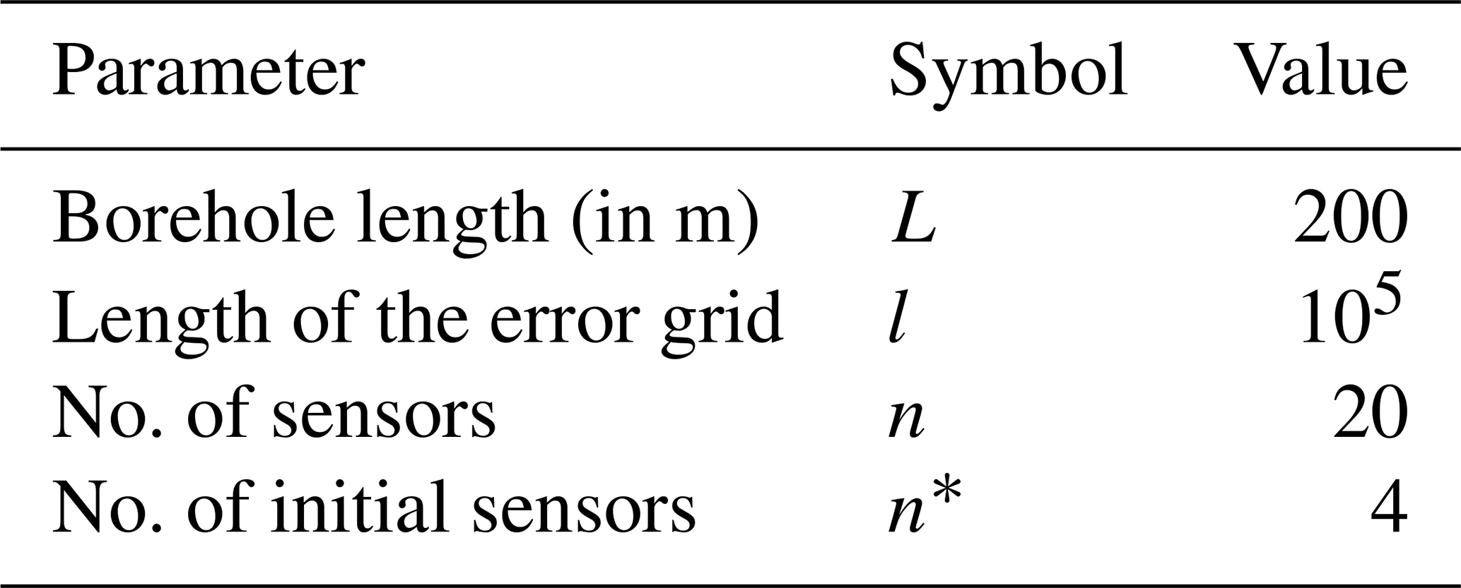
Note: n^* is used only in Algorithm 2.

3 Results

3.1 Comparative analysis of linear, exponential and greedy optimal sensor placements for borehole thermometry

We first compare the performance of linear, exponential, and greedy optimal sensor placements for n=20 sensors for the EDML site, assuming no device error (Fig. 2). Naturally, the sampling error is near zero at the depths where sensors are placed and maximal between sensors. For the linear placement, the maximum sampling error is larger than 100 mK, which occurs between the top two sensors (Fig. 2b, c). For the exponential spacing, the error exceeds 2 mK, which occurs between the deepest two sensors (Fig. 2e, f). The greedy optimal spacing lies between the linear and exponential cases, with larger spacing deeper in the borehole but less than the exponential increase. For the greedy optimal sensor placement, the maximum sampling error is in the top 50 m but is less than 0.2 mK (Fig. 2g–i), and thus an improvement of a factor over 500 compared to the linear spacing.

Strong fluctuations in heat distribution occur closer to the surface and decrease deeper into the ice sheet. Therefore, many studies considered exponential and ad hoc sensor placements with sensors being placed farther apart down the borehole to recover heat distribution effectively. The greedy optimal sensor placements (Fig. 2g) manifests more or less naturally this trend of sensors being placed farther apart down the borehole. The last sensor is an exception due to its fixed location at the very bottom of the borehole.

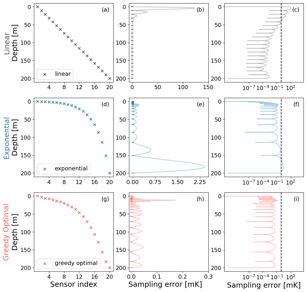
Figure 2 Performance comparison of linear, exponential, and greedy optimal sensor placements in case of EDML, assuming no device error. Panels (a)–(c) are based on linear spacing, (d)–(f) are based on exponential spacing and, (g)–(i) are based on greedy optimal sampling of a set of 20 sensors in a 200 m borehole. The horizontal axis of (a), (d) and (g) shows the index of the sensors, sensor with index-1 is placed at the top and index-20 is placed at the bottom of the borehole. Panels (b), (e) and (h) show the sampling error due to linear, exponential, and greedy optimal sensor placement respectively. Panels (c), (f) and (i) show sampling error in logarithmic scale. The dashed line marks 1 mK in (c), (f), and (i).

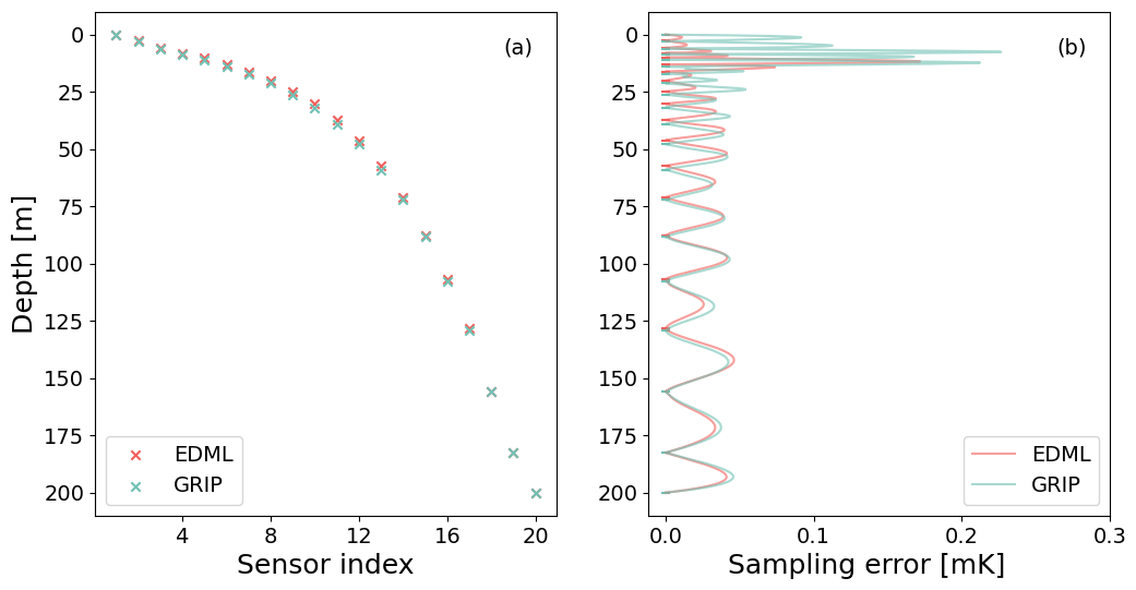
Figure 3 Comparison of the results of greedy optimal sensor placements for the cases of EDML and GRIP, assuming no device error. (a) Depicts the greedy optimal sensor placements for both sites, for a set of 20 sensors in the 200 m boreholes and (b) depicts their respective sampling error.

Interestingly, generally similar results are also obtained for the GRIP ice core site that is characterized by very different site conditions. Comparing the results for both sites in detail, Fig. 3 shows that due to higher accumulation rate of GRIP compared to EDML, the signals are drifted slightly deeper, and therefore the GRIP sensors are placed slightly deeper in the borehole than the corresponding sensors for EDML. The difference between the corresponding sensor locations of the two sites is noticeable (>0.5 m) for sensors placed between ∼ 10 and 130 m depths (Fig. 3a). The sampling error curve appears to be slightly shifted from one another, and the maximum sampling errors of EDML and GRIP are ∼ 0.2 mK (Fig. 3b).

3.2 Dependence of sampling error on the number of sensors used for borehole thermometry

To evaluate the dependence of sampling error on the number of sensors used in the borehole sensor placement, we generate linear, exponential, and greedy optimal sensor placements for n=5 to 20 sensors, assuming initially no device error. For the EDML site, as expected, the maximum sampling error decreases with the increasing number of sensors for all three types of sensor placement (Fig. 4a). Similar results are also observed in the case of GRIP (Fig. B2a in Appendix B).

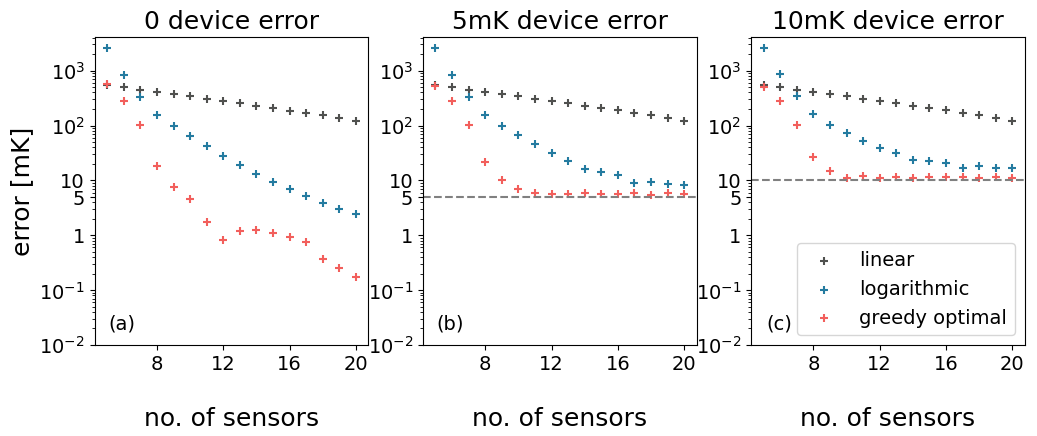
Figure 4 The sampling of linear, exponential and greedy optimal sensor placements with and without device error were computed for 5 to 20 sensors for EDML. Maximal sampling errors without device error (σ_d=0) (a), with 5 mK device error (σ_d=5 mK) (b) and with 10 mK device error (σ_d=10 mK) (c) are given. The number of sensors used in sensor placement is denoted on the horizontal axis of (a), (b) and (c).

We further investigate the influence of a device error on the sampling error. We again generate linear, exponential, and greedy optimal sensor placements for n=5 to 20 sensors, assuming device error of standard deviation σ_d=5 and 10 mK (Fig. 4b, c). The trend of maximum sampling error decreasing monotonically with increasing number of sensors is observed for linear and exponential sensor placement, but not reduced to the device error (σ_d line) with 20 sensors. In the case of greedy optimal sensor placement, this trend is observed until the error is in the range of the device error and then the error continues to be in that range with further increase in number of sensors (Fig. 4b, c). Considering that the sensors have device error, it is clear that the device error of the sensors influences the sampling error. The greedy optimal sensor placements outperformed linear and exponential spacing of sensors as it reduces the maximum sampling error to the range of device error with fewer sensors.

Assuming the sensors have device error, it is important to understand if we can reduce the number of sensors and get good results. As mentioned before, both linear and exponential sensor placement was not able to reduce the sampling error to the range of device error with 20 sensors. The sampling error is not reduced below 100 mK with linear sensor placements considering device error of standard deviation σ_d=5 and 10 mK. For exponential sensor placement the sampling error is not reduced below 8 and 16 mK respectively, when device error of standard deviation σ_d=5 and 10 mK is considered. It is evident that only half the number of sensors is required by greedy optimal sensor placement to reduce the sampling error to the close vicinity of the given σ_d, when compared to respective linear and exponential placements (Fig. 4b, c). GRIP also showed similar results when analyzing the influences of device errors (Fig. B2b, c).

To assess the reliability of greedy optimal sensor placement with fewer sensors, we tested one-by-one sensor failures for sets ranging from 11 to 20 sensors. For each set, we recorded the highest sampling error resulting from the failure of any single sensor, and plotted this maximum error to evaluate performance (Fig. D1 in Appendix D). The greedy optimal placement resulted in the lowest error for all cases and the sampling errors remained within 30 mK when 15 or more sensors (with a sensor failure) are used. In contrast, for the other placement strategies, even with 20 sensors the maximum error under a single sensor failure reached about 60 mK for exponential placements and exceeded 250 mK for linear placements (Fig. D1).

4 Discussion

We found that the greedy optimal sensor placement for borehole temperature measurements provides more informative data than linear or exponential sensor placements, as it enables measurement of the full borehole temperature profile with higher precision and fewer sensors. Here, we review the factors that affect the optimal sensor placement, examine the associated uncertainties, choice of device error, and discuss the broader implications of our findings.

4.1 Numerical uncertainty of greedy optimal sampling algorithm

The greedy optimal sensor placements using Algorithm 2 determines the final sensor placement $\stackrel{\mathrm{‾}}{{\mathit{Z}}_{\mathrm{S}}}$ by an averaging over a larger number of sensor placements that correspond to different sets of initial sensor positions, see Sect. 2.2.2. This averaging is done for robustness reasons. While each individual sensor placement Z_S fulfills optimality properties, their geometric average does not have to be optimal. Therefore, it is of interest to analyze how strongly the averaged sensor placement deviates from the best possible, non-averaged sensor placement and whether averaging over a larger set influences the result.

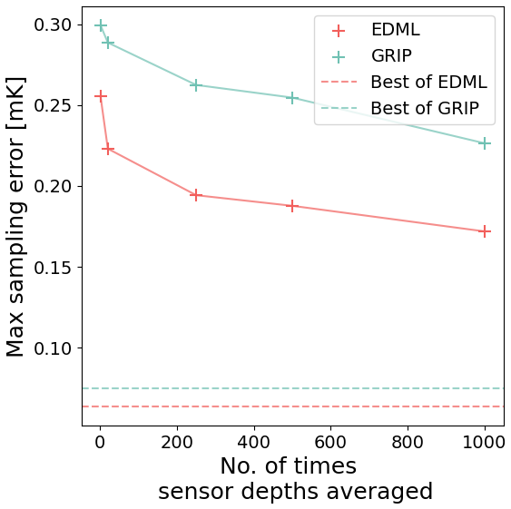
Figure 5 Numerical uncertainty handling of greedy optimal sampling. The obtained maximum sampling error is plotted against the number of greedy optimal sensor placement sets (Z_S), over which the final placement is averaged. The dashed lines represents the best-case sampling error for EDML and GRIP which is the minimum of the maximum sampling errors across the 1000 distinct sensor placement.

We analyze the maximum sampling error of the greedy optimal sensor placement averaged with 1, 20, 250, 500, and 1000 sets of sensor placements. The best case of sampling error is calculated as the minimum of the maximum sampling errors of each of the 1000 distinct sensor placement sets. The maximum sampling error of averaged greedy optimal sensor placement is observed to be decreasing (towards the best case) with increasing the number of sets used in averaging (Fig. 5). Although the maximum sampling error remains significantly higher than the best-case error, the absolute differences, at less than 0.3 mK, are negligible compared to the variations between different sampling strategies or the device error.

4.2 Sensitivity on past climate and ice borehole site properties

To better understand the factors influencing optimal sensor spacing, we conducted a sensitivity study to examine the impact of extreme surface temperature histories and site conditions on our results. In addition to the “realistic” parameter sets used previously, we include one case where the surface temperature history exhibits no trend, only stochastic variability (PA=0, β=0.6), and another case dominated by a warming trend (PA=3, β=0.6), which is stronger than trends currently assumed in the literature or found in state-of-the-art climate model simulations (Jones et al., 2016).

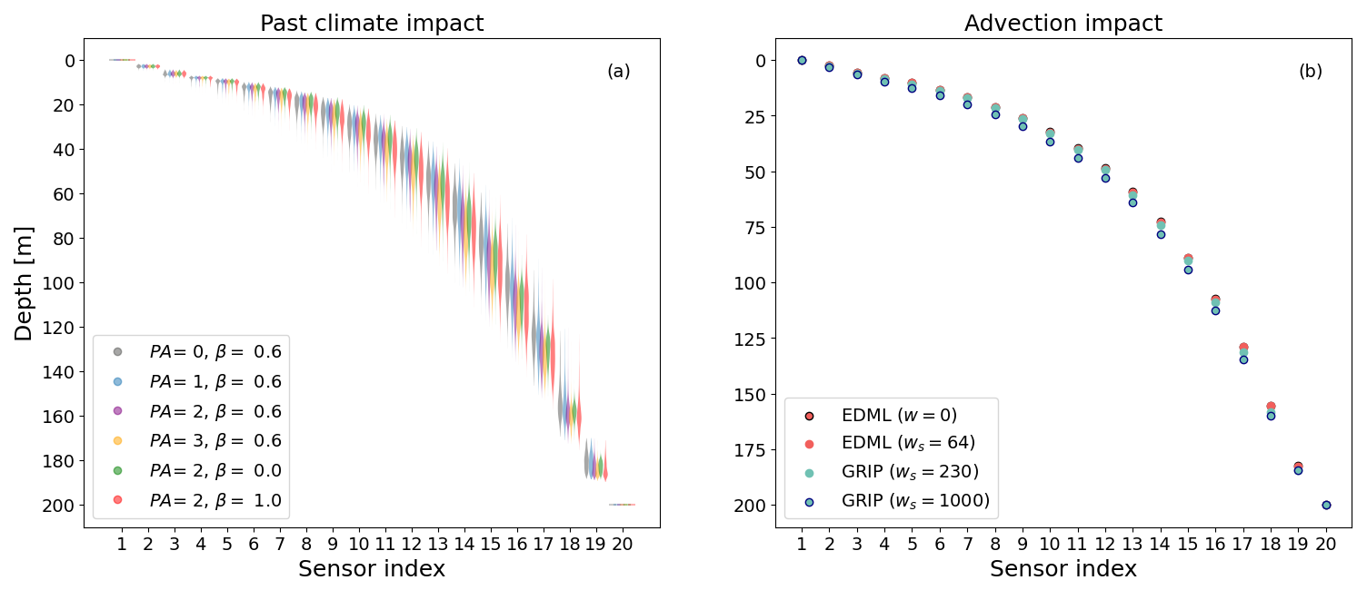
Figure 6 Greedy optimal sensor placements' sensitivity to the surface temperature time series and the accumulation rate that determines the advection. The distribution of the 20 sensor locations computed for different extreme cases of input temperature time series with respect to EDML are shown in (a). Greedy optimal sensor placements for EDML with w_s=64 mm yr⁻¹ and without advection (w=0), and GRIP with its given w_s as 230 mm yr⁻¹ and very high advection (w_s=1000 mm yr⁻¹) are shown in (b). Impact of advection is analyzed using surface temperature time series with PA=2 and β=0.6 (see Sect. 2.3.2).

In contrast to our earlier analysis, we present the full distributions of sensor placements for each of the different types of surface temperature time series. We modified the Algorithm 2 such that we generate greedy optimal sensor placements (for computational efficiency reasons, we only averaged over 20 sets of Z_S in this analysis) for each of the 1000 surface temperature time series of a particular type and thus the distribution of sensor placements with respect to that particular type of surface temperature time series is obtained.

Interestingly, the distributions of 1000 sensor locations generated for the six types of surface temperature time series mostly overlap at the respective sensor indices (Fig. 6a). Even the extreme parameter sets for surface temperature have minimal influence on the results. This insensitivity indicates that sensor placement is primarily determined by the properties of the advection-diffusion equation rather than by any specific surface temperature history.

The primary factor varying between different ice core locations is the snow accumulation rate, which ranges from as little as 30 mm yr⁻¹ on the East Antarctic Plateau to more than 1 m yr⁻¹ in coastal regions. This directly affects the advection term. Additionally, site conditions influence the diffusion term by affecting the density and temperature profiles.

To investigate these influences, we conduct another sensitivity study. In addition to the actual cooler Antarctic EDML and warmer Greenlandic GRIP conditions, we examine two extreme parameter sets: EDML without advection and GRIP with very high advection (w_s=1000 mm yr⁻¹). For surface temperature, we use the standard parameter set (β=0.6, PA=2.0), as we have shown above that the results are not sensitive to this choice.

We find that for all surface conditions studied, the overall shape of the sensor placement is similar (Fig. 6b). However, the accumulation rate has a noticeable effect: the optimal sensor locations, as determined by the greedy algorithm in Sect. 2.2.2, shift deeper into the ice sheet as the accumulation rate increases in the borehole simulations (Fig. 6b). In the extreme case of optimal sensor placement with no advection and extremely high advection, the maximum difference reaches up to 6 m. This behavior aligns with the observation that GRIP sensors are placed slightly deeper in the borehole compared to the corresponding EDML sensors (Fig. 3a).

The uncertainty in bottom boundary condition parameterization of ice sheet have minimal impact in borehole temperature at 200 m. The borehole temperature profile simulated using a Dirichlet boundary condition differs slightly from that obtained using a Neumann boundary, but the effect on optimal sensor placements are undetectable. Greedy optimal sensor placements do not depend on the absolute temperature, but on the variations of the temperature across borehole depth. Therefore, according to our methodology, the difference in borehole temperature profile simulations due to different basal boundary conditions of the ice sheet, does not affect the sampling error, as it is not contributing to the uncertainty budget we are assessing.

4.3 Device error range in ice borehole thermistors

The device error values assumed in this study (5 and 10 mK) fall within the typical range reported for borehole thermistors in glaciological applications. For example, precision values range from around 0.5 mK when using a single thermistor on a winch in high-end systems (Clow et al., 1996) to approximately 30 mK in simpler thermistor chain setups (Muto et al., 2011) while accuracy typically lies in the range of 3–30 mK. Our results show that greedy optimal sampling can reduce the sampling error to a level comparable to these typical device errors, particularly when only a limited number of sensors are used.

4.4 Implications

The proposed ice borehole sensor placement method, utilizing greedy optimal sampling, utilizes the understanding of how heat is distributed in the ice borehole and incorporates our knowledge on potential past climate states.

This approach has broad applicability and can directly be applied for shallow ice borehole thermometry spanning the Holocene period. Given the robustness of our results to variations in site-specific conditions and climate history (e.g., stochastic variability or pronounced trends), already using the proposed sensor spacing is likely to offer substantial improvements over ad hoc placements, even when applied to locations other than those explicitly analyzed in this study. Rerunning our algorithm for specific sites and specific prior knowledge on potential past climate histories is straightforward and has the advantage of also providing the uncertainty caused by using only a finite set of sensors.

For boreholes extending to the bottom of an ice sheet, for example for the estimation of geothermal heat flux (Colgan et al., 2023), the spacing will change near the basal regions and the sensitivity to prior information on the bottom heat flux needs to be tested. For studies encompassing time periods extending beyond the Holocene, such as glacial-interglacial cycles and orbital-scale variations, a revised set of surface temperature histories should be used to account for these longer-term climatic oscillations and depending on the site conditions, the forward model has to be extended with an ice-flow model (Salamatin, 2000).

The greedy optimal approach to sensor placement can further be extended to other problems such as terrestrial boreholes or boreholes in permafrost areas (Groenke et al., 2024) or the measurement of temperature profiles in sea ice (Zuo et al., 2018) using adapted forward heat transfer models. Expected phase changes (e.g., in permafrost) or vertically heterogeneous thermal properties could be incorporated into the forward model, allowing sensor positions to be optimized nonetheless.

5 Conclusion

We propose a greedy strategy for placing sensors in ice boreholes to maximize the informativeness of temperature sensor measurements. Unlike ad hoc, linear and exponential sensor placements, where sensors are positioned as a function of depth, our method determines sensor locations by accounting for the subsurface heat distribution influenced by surface temperature diffusion and advection. Exponential sensor placements, which space sensors farther apart down the ice borehole, are found to outperform linear sensor placements. This is because stronger vertical gradients in heat distribution occur closer to the surface and gradually diminish deeper into the ice sheet. Compared to exponential sensor placement, our simulations demonstrate that the greedy optimal sensor placement increases the informativeness of ice borehole measurements, reducing error by a factor of approximately 10.

Additionally, we analyzed sensor placement while considering the inherent measurement uncertainty (device error). This shows that, under realistic settings, greedy optimal sampling requires only half the number of sensors to minimize sampling error compared to linear and exponential placements. Therefore, we argue that our proposed approach could enable more cost-effective and accurate measurement of ice borehole profiles, making it a promising contribution to the establishment of a continuous subsurface temperature monitoring system.

Appendix A: Heat transfer model parameters

The thermal properties and vertical velocity of the firn/ice is calculated with respect to site specific parameters, which are mean surface temperature (θ_m), basal temperature (θ_b), basal velocity (w_b), accumulation rate (w_s) and thickness of the ice sheet (H).

A1 Thermal properties

The thermal properties include density (ρ), specific heat capacity (c), thermal conductivity (K), and thermal diffusivity (k). The density profile is simulated using the Herron–Langway model (Herron and Langway, 1980; Arthern et al., 2010), which requires surface snow density (ρ_s) in addition to θ_m, w_s and H. The unit of density is kg m⁻³ and it is one of the key inputs to the heat transfer model to calculate heat capacity c and thermal conductivity K. The equations for their calculations are listed below (Cuffey and Paterson, 2010; Muto, 2010; Orsi et al., 2012).

A1.1 Specific heat capacity (c)

Specific heat capacity of ice (c_ice) in J kg⁻¹ K⁻¹ is given by the following equation from Paterson (1994),

$$\begin{array}{}\text{(A1)}& c_{\mathrm{ice}}=\mathrm{152.5}+\mathrm{7.122}T,\end{array}$$

where T is the temperature in Kelvin. Specific heat capacity of firn (c_firn) is calculated from the percentage of ice and air in firn which is given by,

$$\begin{array}{}\text{(A2)}& c_{\mathrm{firn}}=c_{\mathrm{ice}}{\displaystyle \frac{\mathit{\rho }}{{\mathit{\rho }}_{\mathrm{ice}}}}+c_{\mathrm{a}}\left(\mathrm{1}-{\displaystyle \frac{\mathit{\rho }}{{\mathit{\rho }}_{\mathrm{ice}}}}\right),\end{array}$$

where ρ_ice is the density of ice (917 kg m⁻³) and c_a (1005 J kg⁻¹ K⁻¹) is the specific heat capacity of dry air.

A1.2 Thermal conductivity (K)

The temperature-dependent thermal conductivity of ice (K_ice) in W m⁻¹ K⁻¹ is given by

$$\begin{array}{}\text{(A3)}& K_{\mathrm{ice}}=\mathrm{2.22}(\mathrm{1}-\mathrm{0.0067}T),\end{array}$$

where T is temperature in °C. Thermal conductivity of firn (K_firn) is given by

$$\begin{array}{}\text{(A4)}& K_{\mathrm{firn}}=K_{\mathrm{ice}}({\displaystyle \frac{\mathit{\rho }}{{\mathit{\rho }}_{\mathrm{ice}}}}{)}^{{\mathit{\alpha }}^{\prime }-{\mathit{\beta }}^{\prime }\left(\frac{\mathit{\rho }}{{\mathit{\rho }}_{\mathrm{ice}}}\right)},\end{array}$$

where α^′ and β^′ are site specific coefficients. We used ${\mathit{\alpha }}^{\prime }=\mathrm{2.4634}$ and ${\mathit{\beta }}^{\prime }=\mathrm{0}$ for EDML which was used by Muto (2010) for the site NUS07-2, and ${\mathit{\alpha }}^{\prime }=\mathrm{2}$ and ${\mathit{\beta }}^{\prime }=\mathrm{0.5}$ for GRIP (Muto, 2010).

A2 Vertical velocity (w)

As in Muto (2010), the velocity profile is computed using the equation from (Goujon et al., 2003), which is based on the ice velocity model by Lliboutry (1979). Using a relative vertical coordinate $\mathit{\zeta }=z/H$, where H is the ice sheet thickness, w(ζ) is given as

$$\begin{array}{}\text{(A5)}& \begin{array}{rl}w\left(\mathit{\zeta }\right)& ={\displaystyle \frac{\mathit{\rho }}{{\mathit{\rho }}_{\mathrm{ice}}}}[w_{\mathrm{s}}-(w_{\mathrm{s}}-w_{\mathrm{b}}\left)\right({\displaystyle \frac{m+\mathrm{2}}{m+\mathrm{1}}}\mathit{\zeta })\\ & \cdot (\mathrm{1}-{\displaystyle \frac{{\mathit{\zeta }}^{m+\mathrm{1}}}{m+\mathrm{2}}})].\end{array}\end{array}$$

The constants w_s and w_b are the vertical velocity at the surface and at the base of the ice sheet, respectively. w_s is assumed to be equal to the accumulation rate and w_b is the basal melting rate. m is the shape parameter of the vertical velocity profile. We use m=11 for EDML, and m=10 for GRIP.

Appendix B: Sensor placements for GRIP

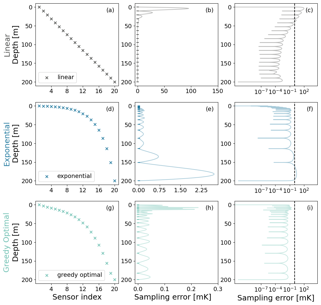
Figure B1 Performance comparison of linear, exponential, and greedy optimal sensor placements in case of GRIP, assuming no device error. Panels (a)–(c) are based on linear spacing, (d)–(f) are based on exponential spacing and, (g)–(i) are based on greedy optimal sampling of a set of 20 sensors in a 200 m borehole. The horizontal axis of (a), (d) and (g) shows the index of the sensors, sensor with index-1 is placed at the top and index-20 is placed at the bottom of the borehole. Panels (b), (e) and (h) show the sampling error due to linear, exponential, and greedy optimal sensor placement respectively. Panels (c), (f) and (i) show sampling error in logarithmic scale. The dashed line marks 1 mK in (c), (f), and (i).

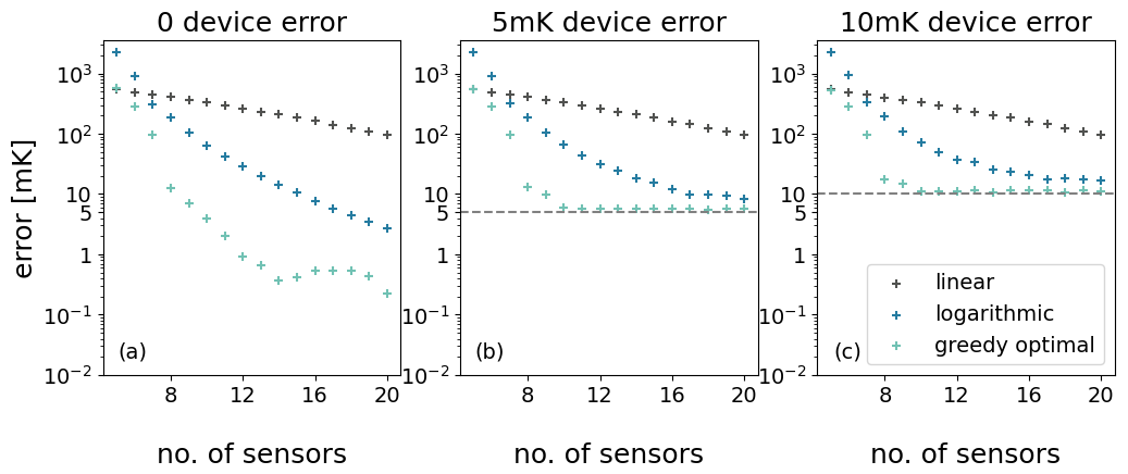
Figure B2 The sampling of linear, exponential and greedy optimal sensor placements with and without device error were computed for 5 to 20 sensors for GRIP. Maximal sampling errors without device error (σ_d=0) (a), with 5 mK device error (σ_d=5 mK) (b) and with 10 mK device error (σ_d=10 mK) (c) are given. The number of sensors used in sensor placement is denoted on the horizontal axis of (a), (b) and (c).

Appendix C: Interpolation function

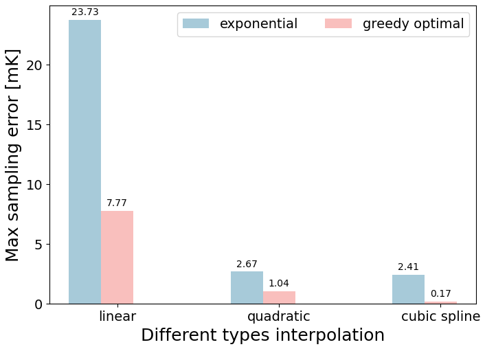
Figure C1 The maximum sampling error of exponential and greedy optimal sensor placements with respect to different types of interpolation functions used is shown here. EDML site parameters are used for this analysis.

Appendix D: Sensor failure test

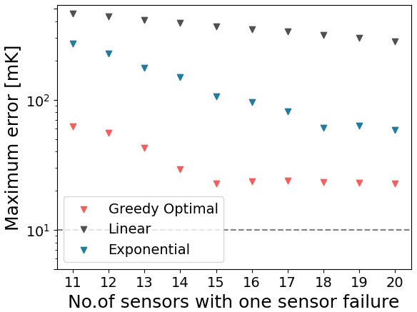
Figure D1 This figure shows the maximal sampling error observed due to single sensor failure for all the three sensor placement strategies of 11 to 20 sensors, each with a device error of standard deviation σ_d=10 mK. The horizontal axis shows the no. of sensors including the failed sensor.