Evaluating data quality and reference instrument robustness: insights of 12 years DI magnetometer comparisons in the Geomagnetic Network of China

Statical analyses were conducted in sequence on 12 sets of geomagnetic instrument comparison data from the Chinese Geomagnetic Network (GNC) between 2010 and 2024. First, by examining these comparison data, it was found that when their cumulative probabilities at the same level, the instrument differences for declination (D) are significantly higher than those for inclination (I). For the same set of instruments, as the frequency of observer changes increases, the instrument differences for D increase, while no significant change was observed for I. This indicates that inter-observer differences have a notable impact on D, primarily due to the complexity of aligning the azimuth marks and levelling instruments. Second, though a multi-source error uncertainty analysis, including instrument error, operator related error, pillar correction error and so on, the systematic differences between the reference fluxgate theodolite and the test instruments were quantified. The operator related errors of D and I were successfully separated and consistent with the observed experimental results, confirming that operator related error is the primary factor contributing to instrument differences. The analysis also validated the high stability and reliability of the reference instrument. The former finding can serve as an assessment criterion for network-level numerical quality, while the latter can be used to verify the long-term stability of the reference instrument.

1 Introduction

In geomagnetic observatories, variometers are employed to record continuous variations of the geomagnetic field. These variations are subsequently converted into absolute geomagnetic field values through the addition of baseline values derived from absolute measurements (Jankowski and Sucksdorff, 1996). This calibration process renders absolute measurements critical for ensuring the quality of continuous absolute geomagnetic data. However, the difference of absolute instruments between different observatories make systematic instrument comparisons as an essential component of modern geomagnetic observation systems.

Contemporary absolute measurements primarily utilize two high precision instruments: (i) fluxgate theodolites (designated as Declination Inclination Magnetometers, DIMs) for measuring declination (D) and inclination (I), and (ii) proton magnetometers for total field intensity (F) determinations. While technological advancements have reduced the required frequency of instrument comparisons, such calibrations remain indispensable for maintaining high quality geomagnetic datasets (Zhang et al., 2024). To standardize global geomagnetic observations, the IAGA Division V Working Group V-OBS has successfully organized over twenty biennial international instrument comparison sessions to date (Loubser, 2002; Masami et al., 2005; Reda and Neska, 2007; Love, 2009; He et al., 2011; Hejda et al., 2013; and so on). In China, the Geomagnetic Network Center (GNC) integrates these comparisons into its quality control framework, serving dual roles as both data hub and quality assurance authority for national observatories (Li et al., 2012; Zhang et al., 2016).

Since the digital transformation of Chinese geomagnetic observatories, the GNC has implemented successive generations of DIMs, including Hungarian MINGEO-DIM, British MAG 01-DIM, Chinese CTM-DIM, Chinese GEO-DIM, Chinese TDJ2E-NM-DIM, etc. It should be noted that the manual operation inherent to these DIM systems introduces two critical uncertainty sources: (i) inter instrument systematic biases, and (ii) operator dependency operational variances. To mitigate these effects and unify observational standards across the geomagnetic network, the GNC has organized instrument (DIMs) comparison measurements almost annually since its digital transformation (He et al., 2019b). Through systematic comparison measurements, each observatory's instrument is calibrated against the reference instrument (DIMs), which is typically designated as the GNC standard and has the characteristics of high measurement accuracy and operational stability, to quantify instrumental differences and achieve nationwide standardization of absolute geomagnetic observations.

The following sections will first briefly introduce the measurement methods used in comparison measurements and the baseline based comparison methods. Then, the research will primarily focus on the historical comparison datasets. Firstly, statistical analysis will be conducted to explore valuable information from the statistical results. Secondly, uncertainty analysis method, widely used in experimental science, is applied to further quantify and extract relevant information from the datasets, to evaluated the uncertainty of the reference instrument relative to the observation results of all instruments in each comparison session. So the long term robustness of the reference instrument can be investigated based on multiyear results.

2 Measurement and comparison methodology

The geomagnetic field, being a vector quantity, requires precise determination of both magnitude and directional components. The DIM, comprising a theodolite integrated with a fluxgate sensor, serves as the standard instrument for determining geomagnetic field direction (declination D and inclination I). The fluxgate sensor, mounted parallel to the theodolite's optical axis, operates on the null detection principle: it generates zero output (assuming zero offset) when aligned perpendicular to the geomagnetic field vector. Directional determination is achieved by identifying sensor null positions, with angular coordinates recorded via theodolite circle readings. The angular between two directions can be determined by computing the difference between their respective readings on the instrument's horizontal circle. This is the fundamental principle of fluxgate theodolite angle measurement.

The fluxgate theodolites are high-precision instruments, but they inevitably contain certain errors, such as misalignment errors between the mechanical axis of theodolite, the optical axis of the telescope, and the magnetic axis of the fluxgate sensor; collimation errors; non-orthogonality errors of the horizontal and vertical axes; uneven graduation errors of the reading circle; index errors; and errors caused by non-zero electronic offsets, which prevent accurate determination of magnetic declination and inclination from a single reading of the horizontal/vertical circle (Lauridsen, 1985; Newitt et al., 1996; Csontos and Šugar, 2024). However, in theory, most of these errors can be eliminated through the four position measurement process, and some of them (two misalignment errors between the fluxgate sensor axis and the optical axis of the telescope in the horizontal/vertical planes, and the offset error of the fluxgate sensor) can be calculated from the measurement results (Bitterly et al., 1984). The specific measurement methods and procedure are described in Appendix A1.

Ensuring high quality geomagnetic observations necessitates systematic verification of inter-instrument differences across observatories. The comparison analysis of absolute measurement instruments constitutes an essential quality assurance measure in geomagnetic monitoring networks. Practical constraints, including limited pillar availability, multiple DIMs, and operator skills proficiency, render synchronous multi instrument comparisons operationally challenging. Modern variometers exhibit high precision performance with quasi constant baseline characteristics under stable operating conditions, while underground observation rooms of geomagnetic observatories (far from cities or villages) can provide such operating conditions, including no influence of magnetic objects, low electromagnetic background noise, indoor annual temperature variation not exceeding 10 °C, daily variation not exceeding 0.3 °C, and so on. The current comparison protocols therefore employ independent absolute measurements followed by baseline value cross validation. The stability and accuracy of baseline values during a single calibration day were investigated by Zhang and Yang (2011), whose study confirmed that baseline values remained stable throughout the calibration period (08:30 to 16:30 local time), with geomagnetic activity exhibiting no significant impact on their accuracy. Consequently, direct comparison of baseline values is a valid approach for completing the analysis. The baseline calculation and instrument comparison methodology are presented in Appendix A2.

3 Statistic analysis on comparison datasets

In each instrument comparison, all fluxgate theodolites instruments are brought to a specific observatory with excellent observation environment and compared with the reference instrument designated by the GNC. The reference instrument consists of a Zeiss 010B theodolite and a fluxgate sensor, with accuracies better than 1 arcsec and 0.1 nT, respectively. The other instruments, known as testing instrument, come from 46 observatories of GNC, including five types as mentioned earlier. The locations of all observatories and the specific observatory (code QIX highlighted in blue) for comparison are shown in Fig. 1. The codes of all the observatories and their corresponding instrument types, as well as the number of times each instrument participated in comparison and the number of operators (with non-repeated counts), are listed in Table 1. The No. 0 in Table 1 is the reference instrument. The relevant information and parameters for five types of fluxgate theodolites are provided in Table 2.

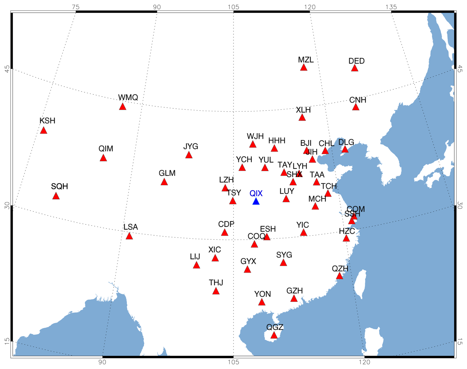
Figure 1 The observatory locations of GNC.

Table 1 The list of instrument type and its observatory.

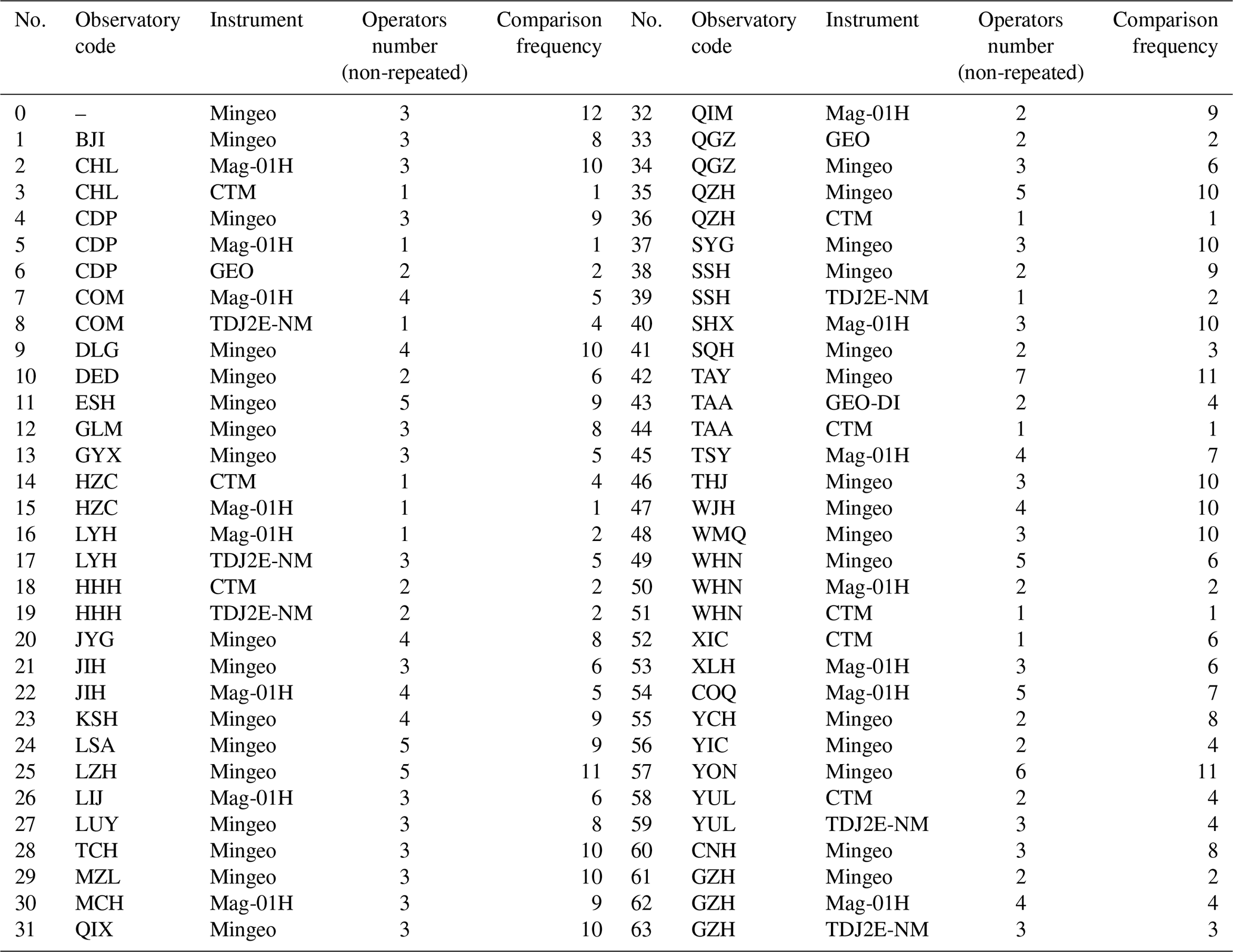
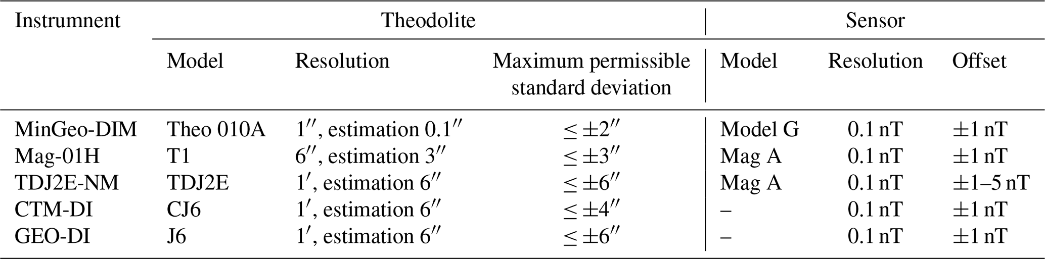
Table 2 The relevant information and parameters of the five fluxgate theodolites.

Based on the aforementioned methodology, the GNC has completed 12 comparisons of DIMs from 2010 to 2024 (no comparison was conducted in 2011, 2013, and 2021), and corresponding datasets have been accumulated. The datasets for comparing all testing instruments with reference instrument are displayed in Fig. 2, where panel (a) and panel (b) respectively illustrate the instrumental differences in declination (ΔU_D) and inclination (ΔU_I). Colored dots in this figure represent measurement results from different years, with vertical coordinates indicating instrumental differences, while the dot sizes indicate the standard deviations of measurements, scaled according to the legend on the right. This graphical representation enables a comprehensive evaluation of observational data quality at both individual instrument and the network levels.

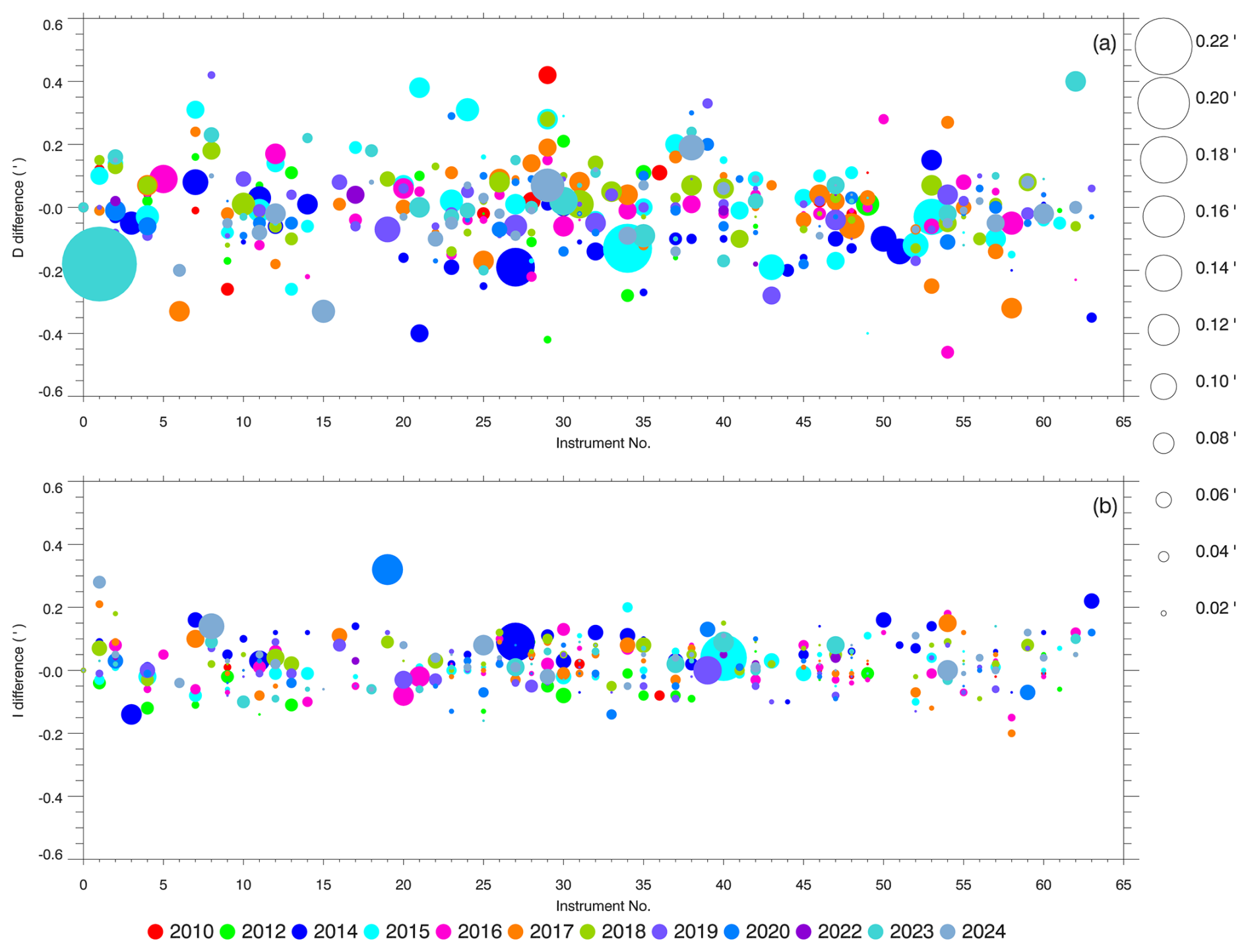
Figure 2 Instrumental differences in (a) declination D and (b) inclination I. The dots represent the instrument differences; the size of the dots is the standard deviation with the scale on the right. The colors indicate different years.

This figures also provide insights into instrument performance and operator proficiency. Small dots with large central values indicate significant instrumental differences, suggesting potential instrument malfunctions or operational issues by personnel. Particularly when the difference of D is relatively large while that of I is small, the most likely cause is the positioning error of the theodolite on the pillar, which also reflects technical shortcomings in observational practices. Conversely, large dots with small central values signify dispersed data, which could arise from instrument related issues (e.g., unclear optical paths affecting reading accuracy) or inconsistent operational practices. More detailed explanations for tracking abnormal information can be found in He et al. (2019b). This graphical approach thus effectively monitors instrument performance and evaluates observational quality across operators.

To assess of network wide data quality, we conducted statistical analyses of all instrument differences, as shown in Fig. 3. The statistical result reveals that declination (D) and inclination (I) measurements approximate normal distributions, with means of 0.00^′ and 0.02^′, and standard deviations of 0.13^′ and 0.07^′, respectively. Approximately 75.1 % of declination and 86.8 % of inclination measurements fall within ±1σ of the mean. When adopting a cumulative probability of 90 % as the evaluation criteria for the entire network, the corresponding instrument differences thresholds are 0.21^′ for D and 0.11^′ for I, indicating excellent consistency among network fluxgate instruments. Notably, declination measurements exhibit greater dispersion than inclination values. This difference stems from the additional azimuth marker alignment required in declination measurements – a process more susceptible to operator error compared to inclination measurements. Another significant source of possible error in declination readings, which is not present in inclination readings, is the accuracy of setting (at 90 or 270°) on the vertical circle.

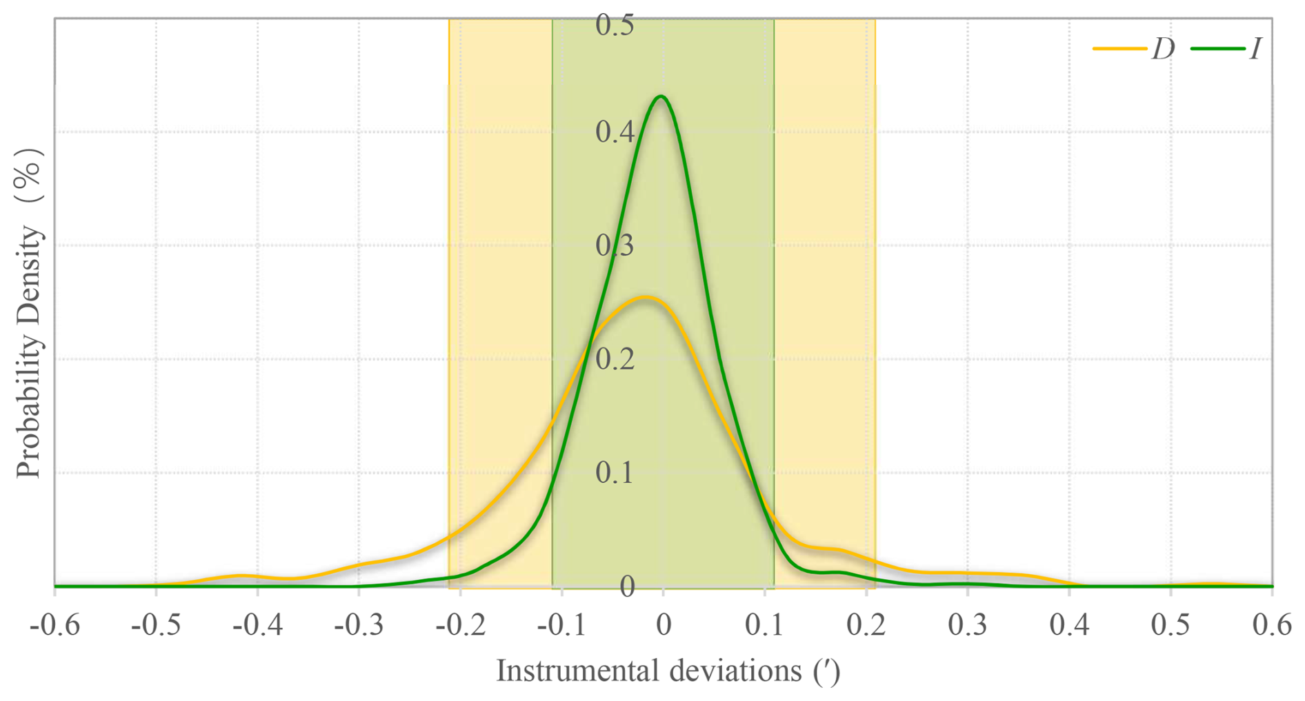
Figure 3 The instrument differences of declination D (orange line) and inclination I (green line).

The dispersion of multiple dots corresponding to the same instrument also reflects its data quality and operation stability. Frequent personnel changes for same instrument have introduced operator dependency errors, manifesting as increased dispersion. To further explore the relationship between frequent personnel changes and the dispersion of instrument differences, the frequency personnel change was defined as the ratio of non-repeated operators to the total number of comparison measurements for each instrument (from Table 1), serving as the x axis, the dispersion degree was represented by the standard deviation of all instrumental differences for each instrument, serving as the y axis. To enhance statistical significance, only instruments that participated in 3 or more comparisons were included in the analysis. As shown in Fig. 4a, the dispersion degree of the instrumental differences increases with the frequent personnel changes, while this phenomenon is less pronounced in Fig. 4b. This indicates that frequent personnel changes increase observational errors and that personnel changes have a greater impact on D than on I. This result is consistent with the conclusion in the previous paragraph that D errors are larger than I errors. It further provides strong evidence supporting the explanation that operator errors primarily arise from the alignment of markers and the level adjustment of the theodolite.

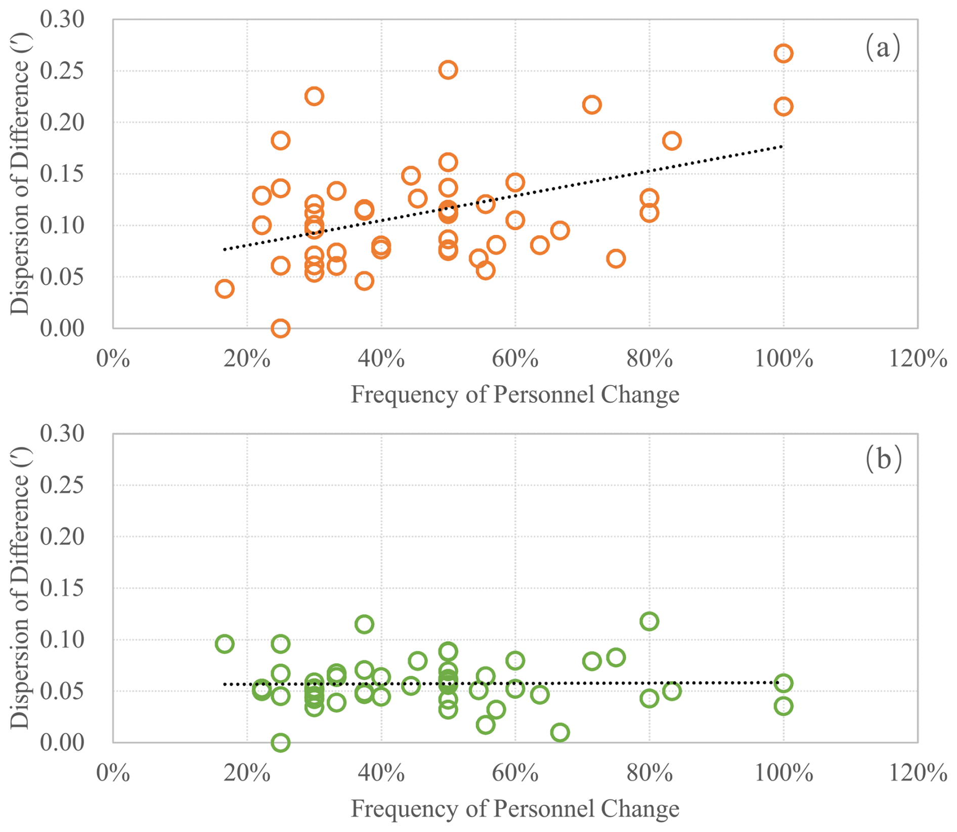
Figure 4 The relationship between frequent personnel changes and the dispersion of instrument differences, (a) declination D, (b) inclination I, and the black dashed line is a linear fitting line.

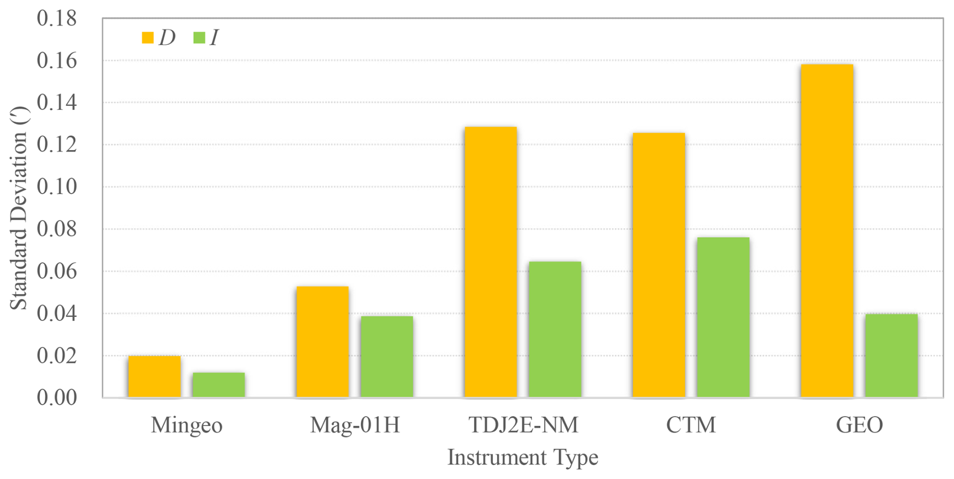
The instrument differences of all 12 years' comparisons were classified to five group based on the instrument type, and the standard deviations were calculated for each group. This was done to simply compare the stability of observational results across different instrument types, as shown in Fig. 5. It can be clearly seen that MINGEO has better stability, followed by Mag-01H and TDJ2E-NM, while the other two have relatively large dispersion, which is directly related to the resolution of the theodolite.

Figure 5 The standard deviation of the instrument differences for five types of instruments.

This simplified comparison measurement provides an efficient mechanism for identifying inter station differences, monitoring instrument performance, and ensuring standardized high quality observations across the network. However, the efficacy of this mechanism critically depends on the precision and accuracy of reference instruments. Beyond routine maintenance and calibration of reference instrument, it is necessary to analyses long term stability and reliability. The following section will evaluate the reference instruments using all comparison measurement data through uncertainty analysis.

4 Uncertainty analysis on comparison datasets

During the comparison process, fluxgate theodolites are employed to observe magnetic declination and inclination. To minimize errors, each observed magnetic declination and inclination is the results obtained after four measurement processes. And the final instrument differences are obtained by comparing the baseline values. However, errors (as mentioned in Sect. 2.1) cannot be completely eliminated and will still exist, which is the main reason for the instrument differences and the source of uncertainty in measurement results. Therefore, the instrument differences defined in this paper are the comprehensive differences of the entire instrument system, representing the differences between results obtained by the instruments after four measurement processes under the assumption of no personnel operation error. The impact of various internal errors of the fluxgate theodolite on the measurement results is already included in the measurement results and is part of the differences of the theodolites, which will not be discussed separately. Then, a quantitative analysis of the error will be conducted based on uncertainty analysis methods.

As described above, the uncertainty analysis in this process encompasses several key error sources, including internal errors of the theodolite, repeatability errors, operator dependency errors (differences between individuals), and pillar correction errors. Environmental interference is excluded from consideration due to controlled laboratory conditions. The uncertainty analysis process and calculation formula applied in the comparison datasets are described in Appendix B.

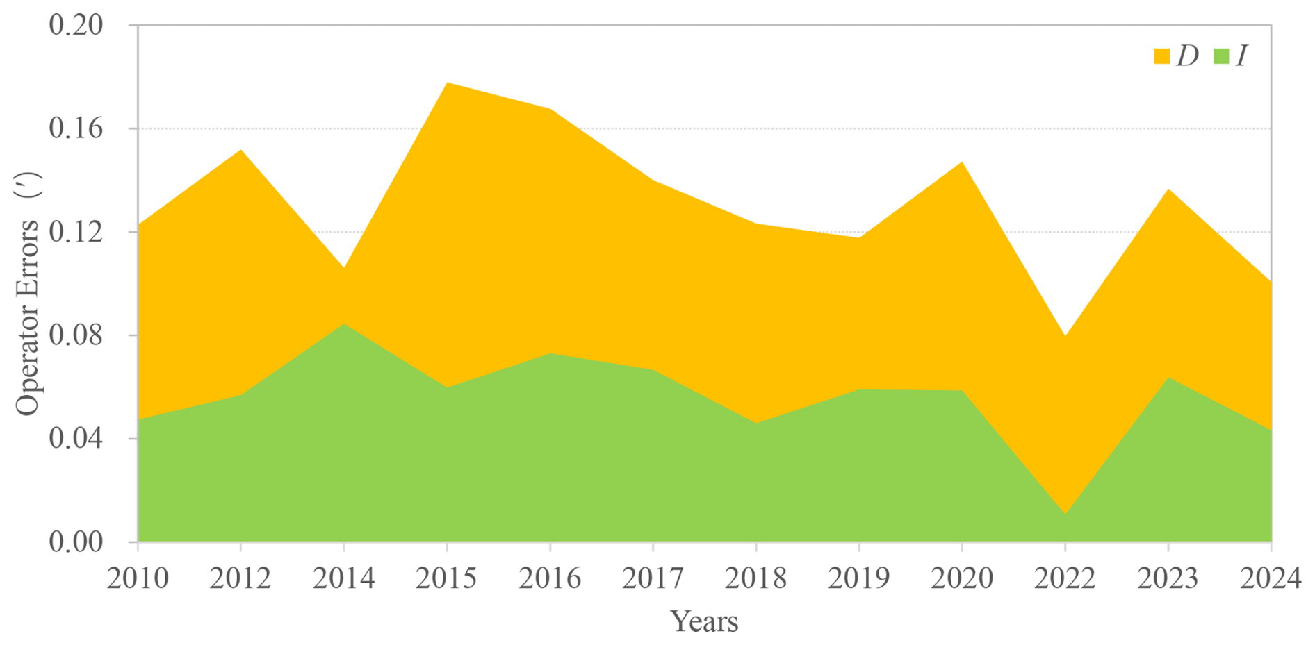
For an instrument comparison, after calculating the synthesized internal uncertainty (u_inst,i) of each instrument, the standard deviation (s_rep,i) and associated Type A uncertainty (u_rep,i) of the repeatability error, as well as the standard deviation (s_between) of all operator-instrument-combinations results, the operator uncertainty (u_oper) can be calculated using Eq. (B7) based on these results. When the above calculation process is repeatedly applied to the results of 12 comparison datasets, 12 operator errors are obtained, as illustrated in Fig. 6. The light orange and light green filled areas represent the differences for D and I, respectively. Results show consistently higher operator dependency errors in declination measurements compared to inclination, with D errors persistently exceeding I values. This difference arises from the additional azimuth marker alignment step, and the accuracy of the vertical circle setting (at 90 or 270°) required for declination measurements, which introduces greater operator variability. The mean operator dependency errors were 0.13^′ for D and 0.06^′ for I, aligning closely with experimental results (0.18^′ for D and 0.08^′ for I) reported by He et al. (2019a), thereby validating the methodology's effectiveness in quantifying operator dependency errors.

Figure 6 Operator dependency errors in Declination (D) and Inclination (I) measurements.

The robustness evaluation of the reference instrument requires quantification of its systematic deviation relative to the true values and associated uncertainties. If each instrument comparison is regarded as an independent measurement experiment, then the average of the measurement results (after correction) from all instruments (excluding the reference instrument) can be taken as the true value of that measurement experiment. Then, the measurement result from the reference instrument can be compared with the true value, and the total uncertainty of the comparison result can be calculated based on the uncertainty formula. In this way, the operational status of reference instruments can be examined. By applying this same process to 12 sets of comparison data, the long-term stability of the reference instrument can be evaluated.

Using the methodology described above, we analyzed 12 years of instrumental difference data for declination (D) and inclination (I). The time series of mean differences (Δ) between the reference instrument and all instruments, along with their uncertainties (u_Δ), are shown in Fig. 7. In this figure, orange and green histograms represent mean differences for D and I, respectively, while curves of corresponding colors indicate twice the uncertainty (2u_Δ). According to the criterion $\left|\stackrel{\mathrm{‾}}{\mathrm{\Delta }}\right|$ ≤ $\mathrm{2}{u}_{\stackrel{\mathrm{‾}}{\mathrm{\Delta }}}$, most mean differences fall within the 2u_Δ range.

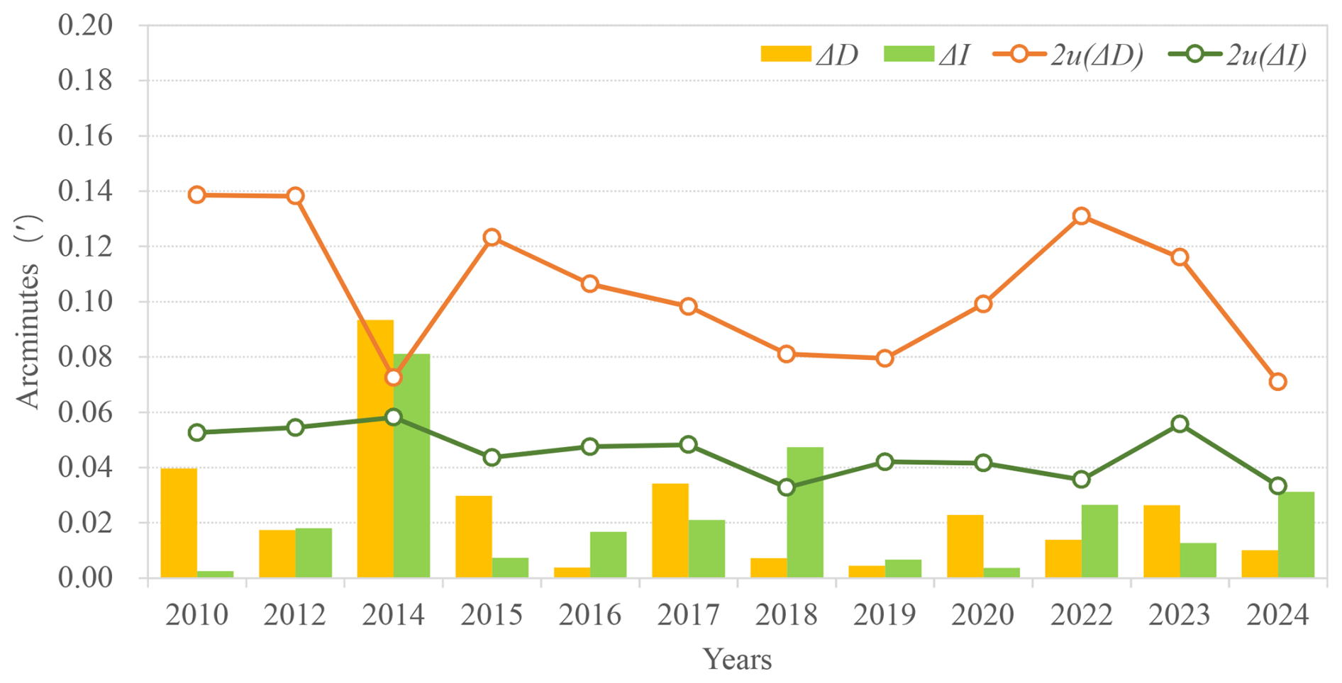
Figure 7 Time Series of Mean Differences and Uncertainties Between Reference and Tested Instruments.

However, mean differences for both D and I exceeded this threshold in 2014. A retrospective review of the raw data revealed no definitive cause for this anomaly. Notably, 2014 involved an observational training program where measurements were conducted by inexperienced personnel, and the definite uncertainty was notably low. This suggests potential transient impacts on the reference instrument. Additionally, the mean difference for D in 2018 slightly exceeded 2u_Δ, though no conclusive explanation has been identified. Nevertheless, the long term mean difference data demonstrate that the reference instrument has maintained stable operation and reliable performance throughout the study period.

Finally, using Eqs. (B16) and (B17), we evaluated the reference instrument's long term stability by calculating the multi years average mean differences and their uncertainties. For declination (D), the average mean difference was $\stackrel{\mathrm{‾}}{{\mathrm{\Delta }}_{\mathrm{D}}}$ = −0.004^′ with an uncertainty of $u_{\stackrel{\mathrm{‾}}{\mathrm{\Delta }D}}$ = 0.054^′. For inclination (I), the values were $\stackrel{\mathrm{‾}}{{\mathrm{\Delta }}_{\mathrm{I}}}$ = 0.022^′ and $u_{\stackrel{\mathrm{‾}}{\mathrm{\Delta }I}}$ = 0.023^′. Applying the criterion $\left|\stackrel{\mathrm{‾}}{\mathrm{\Delta }}\right|$ ≤ $\mathrm{2}{u}_{\stackrel{\mathrm{‾}}{\mathrm{\Delta }}}$ (95 % confidence level), both D and I meet this requirement, confirming the reliability of the reference instrument's long term observational data.

5 Conclusion and outlook

This study systematically analyzed 12 sets of comparison measurement data from the GNC. The research findings demonstrate the critical importance of instrument comparisons in geomagnetic observatory networks, primarily manifested in the following two aspects: (i) the instrument comparison effectively monitors the operational status of instruments at various observatories, assesses the technical proficiency of operators, and enables timely repair and maintenance of problematic instruments; and (ii) the comparison data facilitates the analysis of factors contributing to absolute geomagnetic observation errors, allows for a comprehensive evaluation of data quality across the entire geomagnetic network, and provides a means to assess whether reference instrument meets standards. These assessments also offer valuable references for evaluating the reliability of scientific conclusions derived from geomagnetic data.

The statistical analysis results reveal that when the probability density of instrument differences accumulates to 90 %, the corresponding instrument difference are 0.21^′ (D component) and 0.11^′ (I component), which can serve as evaluation criteria at the network level. The statistical results of the comparison also effectively reflect the factors influencing the declination measurement. Specifically, they reveal that the frequent rotation of operators has a significant impact on the declination observation results, while its effect on the inclination is not as pronounced. This further suggests that operator dependency error is the primary source of error in absolute geomagnetic measurements.

Through uncertainty analysis of multi-source error, the systematic differences between the reference instruments and the test instruments were quantified. The operator dependency errors of D (0.13^′) and I (0.06^′) were successfully separated and consistent with the observed experimental results, confirming that operator dependency error is the primary factor contributing to instrument differences. Notably, operator dependent errors in D are significantly higher than I, which once again proves that D is more susceptible to human factors. A comprehensive evaluation was developed to assess the robustness of reference instrument. By constructing time series of mean differences (Δ) and their uncertainties between the reference instrument and all testing instruments, the long term stability of the reference instrument can be analyzed. The results showed that the data remained stable for a long time without significant drift, and the average of mean differences are −0.004^′ (D) and 0.022^′ (I), both within the 95 % confidence interval. This indicate the reference instrument exhibit high stability and reliability.

However, this approach has limitations. For instance, it overlooks operator instrument interactions and environmental factors (e.g., humidity fluctuations), which may introduce systemic biases. Long term stability analysis also requires extensive multi years comparison data to ensure statistical power, limiting rapid field applications. Future research should focus on model optimization, such as incorporating environmental sensor data to establish temperature/humidity compensation mechanisms or developing automated tools to streamline multi sources uncertainty synthesis. With continuous refinement, this methodology holds promise for advancing standardization and long term stability in geomagnetic observation networks.

Geomagnetic observatories serve as primary facilities for measuring the secular variation of the Earth's magnetic field. The measurement accuracy for directional elements (e.g., declination and inclination) is typically required to be below 0.1^′, while the accuracy for intensity elements (e.g., total field strength) should be within 1nT. Modern instruments, such as the Zeiss 010B fluxgate theodolite, theoretically possess sufficient precision to achieve these targets. However, in practice, attaining such accuracy remains challenging due to various sources of error, particularly operator dependency errors. With advancements in automation and the global adoption of high precision instruments (Rasson and Gonsette, 2011; Gonsette et al., 2017; Hegymegi et al., 2017) in the future, it is anticipated that operator dependency differences will be eliminated, thereby obtaining higher quality geomagnetic observational data.

Appendix A: Measurement procedure and comparison methodology

A1 Measurement procedure

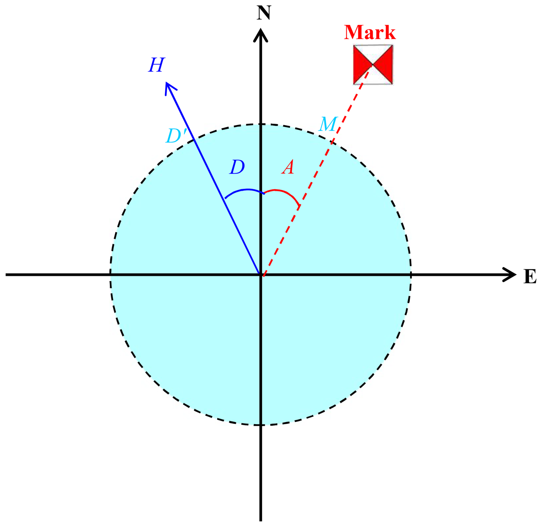
Geomagnetic declination and inclination measurements are performed within the horizontal and magnetic meridional of the theodolite respectively. The declination determination involves two sequential operations: establishing true north orientation and identifying the geomagnetic meridian direction. The true north orientation is calibrated by aligning the telescope's optical axis with a predefined azimuth marker. In order to eliminate errors associated with the optical misalignment of the theodolite, two observations are required to find the true north direction, one with sensor up and the other with sensor down. Finally, the direction of the azimuth marker can be determined through two readings and recorded as M (Fig. A1). As the azimuth value A of the marker known, the true north position can be calculated. Subsequently, the geomagnetic meridian direction is identified by searching the fluxgate null position in the horizontal plane (with the vertical circle maintained at 90 or 270°) and recording horizontal reading (D^′). The geomagnetic declination D is then derived from the differential angular measurement following the formula:

$$\begin{array}{}\text{(A1)}& D=D^{\prime }-M+A.\end{array}$$

Inclination measurements follows analogous procedures and is carried out in the magnetic meridional plane derived from the previous declination measurements, while also within the vertical reference provided by the gravity field through the theodolite suspension system.

Figure A1 Measurement principle of the declination.

The measurement procedure follows the guide published by IAGA (Newitt et al., 1996), and the specific description of the four positions observation can refer to the observation steps in Csontos and Šugar's (2024) paper. The declination measurement protocol is preceded and followed by sensor up and down azimuth marker readings and then involves four configurations: (i) telescope East/sensor up (D₁), (ii) telescope West/sensor down (D₂), (iii) telescope East/sensor down (D₃), and (iv) telescope West/sensor up (D₄). Four different position observations can eliminate errors associated with theodolite optics, sensor misalignment and electronics offset (Csontos and Šugar, 2024). Then final declination value is derived through arithmetic averaging:

$$\begin{array}{}\text{(A2)}& D^{\prime }=\left(D_{\mathrm{1}}+D_{\mathrm{2}}+D_{\mathrm{3}}+D_{\mathrm{4}}\right)/\mathrm{4}+\mathrm{90}\mathit{°}.\end{array}$$

An analogous procedure governs inclination measurement, with positional configurations: (i) telescope North/sensor up (I₁), (ii) telescope South/sensor down (I₂), (iii) telescope North/sensor down (I₃), and (iv) telescope South/sensor up (I₄). The inclination is calculated as:

$$\begin{array}{}\text{(A3)}& I=\left(I_{\mathrm{1}}+I_{\mathrm{2}}-I_{\mathrm{3}}-I_{\mathrm{4}}\right)/\mathrm{4}+\mathrm{90}\mathit{°}.\end{array}$$

This methodology effectively compensates for fluxgate sensor optical axis misalignment (Deng et al., 2010).

Two distinct circle reading techniques are employed: the null method (exact zero point detection) and the offset method (near zero linear region utilization). As demonstrated by Xin et al. (2003), Lu et al. (2008), and Deng et al. (2011), modern theodolites' high output linearity enables equivalent accuracy between methods, even with minor operator induced magnetic interference, making the offset method preferable for operational efficiency.

By using the geomagnetic declination (D), inclination (I), and the total magnetic intensity (F) measured by the proton magnetometer, all the absolute components of the Earth's magnetic field can be calculated. This will facilitate the subsequent baseline calculations of variometer for all components (such as east, north, and vertical directions).

A2 Baseline calculation and comparison

The formula for calculating the baseline value of component W, as defined in the INTERMAGNET Reference Manual (St-Louis, 2024), is presented below:

$$\begin{array}{}\text{(A4)}& W_{\mathrm{B}}\left(k\right)=W_{\mathrm{O}}(i:j)-W_{\mathrm{R}}\left(k\right),\end{array}$$

where (i:j) is the time interval (typically minutes) for measurement, (k) is the kth time, the average time of interval (i:j), W_O(i:j) is the absolute field value for the time interval (i:j), W_R(k) is the variometer recorded value at time k, and W_B(k) is the derived baseline value.

When absolute measurements are performed on different pillars, baseline correction to the reference pillar requires pillar differences. The generalized formulation for component W correction is:

$$\begin{array}{}\text{(A5)}& \mathrm{\Delta }{U}_{\mathrm{SO}}=W_{\mathrm{BS}}-W_{\mathrm{BO}}+\mathrm{\Delta }{W}_{\mathrm{SO}},\end{array}$$

where S is the reference pillar designation, O is the non-reference observation pillar, W_BS and W_BO are respectively the baseline values from reference and observation pillars, ΔU_SO is the final instrument difference, ΔW_SO is the pillar difference, which represents the difference between the base pillar and the reference pillar. These pillar differences were measured before the observatory was put into operation and remeasured before each comparison.

There are two main ways to determine the pillar difference: the direct simultaneous measurements and indirect baseline values comparison. If two or more instruments are available for measurements, the direct method can be applied, and the pillar difference can be calculated by the following Eq. (A6):

$$\begin{array}{}\text{(A6)}& \mathrm{\Delta }{W}_{\mathrm{SO}}=\left[\left(W_{\mathrm{ps}}+W_{\mathrm{qs}}\right)-\left(W_{\mathrm{po}}+W_{\mathrm{qo}}\right)\right]/\mathrm{2},\end{array}$$

where p, q denote the different instruments and s, o represent the standard pillar and other observation pillars, respectively. W_ps and W_qo represent the baseline value of instrument p on standard pillar and the baseline value of instrument q on other pillars, respectively. ΔW_SO is the pillar difference between the standard pillar and other pillars.

If only one instrument is available, the indirect method can be used to calculated the pillar difference using the follow Eq. (A7):

$$\begin{array}{}\text{(A7)}& \mathrm{\Delta }{W}_{\mathrm{SO}}=W_{\mathrm{ps}}-W_{\mathrm{po}}.\end{array}$$

This methodology enables cross comparisons of fluxgate theodolite through pillar reference baseline correction. The obtained difference values ΔU_SO provide quantitative evaluation parameters for assessing absolute observation data quality across participating instruments.

Appendix B: Application of uncertainty in comparison datasets

The true value is the absolute, unbiased value of the measured physical quantity, which is typically unattainable directly in most cases. It can usually be represented by the arithmetic mean of sufficiently repeated measurement data, while uncertainty characterizes the dispersion of the measured value, indicating the range within which the true value may lie, including Type A and Type B standard uncertainties. Type A uncertainty is a type of uncertainty evaluated through statistical methods (e.g., standard deviation of repeated measurement data) to assess the reliability and dispersion of measurement results. Its evaluation relies on the statistical analysis of repeated experimental data. While Type B uncertaintyis based on non-statistical methods (e.g., instrument calibration certificates, empirical formulas, or known error limits), often combined with prior information or professional judgment (ISO/IEC GUIDE 98-3:2008, International Organization for Standardization and International Electrotechnical Commission, 2008).

B1 Uncertainty of fluxgate theodolite error

The fluxgate theodolite consists of two primary components: the theodolite and the fluxgate sensor. Therefore, its uncertainty of internal error also need to be calculated separately for each component. For the theodolite component, errors usually follow a normal distribution, while for the fluxgate sensors, errors raised from the limited resolution (ε = 0.1 nT) of the liquid crystal display follow a uniform distribution. Both can be evaluated using the Type B standard uncertainty according to ISO/IEC GUIDE 98-3:2008. Typically, the maximum permissible standard deviation of horizontal and vertical angles for one measurement cycle is considered as the standard for theodolite level classification based on GB/T 3161-2015 (General Administration of Quality Supervision, Inspection and Quarantine of the People's Republic of China, and Standardization Administration of China (SAC), 2015). This can be used as a parameter to evaluate the theodolite. Therefore, the first step is to consult the theodolite's relevant manual and obtain its parameter. Based on the data in Table 2, the Type B standard uncertainty for theodolite component and fluxgate sensor can be calculated using Eqs. (B1) and (B2) from ISO/IEC GUIDE 98-3:2008., respectively.

$$\begin{array}{}\text{(B1)}& u_{\mathrm{b}\mathrm{1}}=\mathit{\delta }/\mathrm{3},\end{array}$$

where δ is the maximum permissible standard deviation.

$$\begin{array}{}\text{(B2)}& u_{\mathrm{b}\mathrm{2}}=\mathit{\epsilon }/\sqrt{\mathrm{3}},\end{array}$$

where ε is the limited resolution.

In addition, there may be other uncertainties that affect the observations, such as magnetic contamination of the theodolite body. Although these effects are difficult to quantify, they increase the uncertainty of the measurement results and will also be reflected in the measurement results. So the synthesized internal uncertainty for each instrument is computed as the root sum square of two elements, as shown in Eq. (B3):

$$\begin{array}{}\text{(B3)}& u_{\mathrm{inst},i}=\sqrt{u_{\mathrm{b}\mathrm{1},i}^{\mathrm{2}}+u_{\mathrm{b}\mathrm{2},i}^{\mathrm{2}}}.\end{array}$$

B2 Uncertainty of repeatability and operator error

Operators from different observatories performed repeated observations (i.e., 6–8 sets of results) using their own instruments during each instrument comparison, thereby obtaining results of the operator-instrument combination. Based on these results, the standard deviation (s_rep,i) and associated Type A uncertainty (u_rep,i) of the repeatability error for each operator-instrument-combination can be calculated using Eq. (B4):

$$\begin{array}{}\text{(B4)}& {\displaystyle }{u}_{\mathrm{rep},i}={\displaystyle \frac{s_{\mathrm{rep},i}}{\sqrt{N}}},\text{(B5)}& {\displaystyle }{s}_{\mathrm{rep},i}=\sqrt{{\displaystyle \frac{\mathrm{1}}{N-\mathrm{1}}}{\sum }_{k=\mathrm{1}}^N{\left(x_{i,k}-{\displaystyle \frac{\mathrm{1}}{N}}{\sum }_{k=\mathrm{1}}^N{x}_{i,k}\right)}^{\mathrm{2}}},\end{array}$$

where x is the baseline value calculated according to Eq. (A4) and corrected for pillar difference, N is the number of baseline values for each instrument.

Since multiple operator-instrument-combinations from different observatories are involved in an instrument comparison, the standard deviation (s_between) of all operator-instrument-combinations results can be calculated following Eq. (B6). It includes both the internal error of theodolite and the operator error, so the operator uncertainty (u_oper) can be derived by subtracting the averaged instrumental uncertainties, as shown in Eq. (B7):

$$\begin{array}{}\text{(B6)}& {\displaystyle }{s}_{\mathrm{between}}=\sqrt{{\displaystyle \frac{\mathrm{1}}{N-\mathrm{1}}}{\sum }_{i=\mathrm{1}}^N{\left({\stackrel{\mathrm{‾}}{x}}_i-\stackrel{\mathrm{‾}}{\stackrel{\mathrm{‾}}{x}}\right)}^{\mathrm{2}}},\stackrel{\mathrm{‾}}{\stackrel{\mathrm{‾}}{x}}={\displaystyle \frac{\mathrm{1}}{N}}{\sum }_{i=\mathrm{1}}^N{\stackrel{\mathrm{‾}}{x}}_i,\text{(B7)}& {\displaystyle }{u}_{\mathrm{oper}}=\sqrt{s_{\mathrm{between}}^{\mathrm{2}}-{\displaystyle \frac{\mathrm{1}}{N}}{\sum }_{i=\mathrm{1}}^N{u}_{\mathrm{inst},i}^{\mathrm{2}}},\end{array}$$

where $\stackrel{\mathrm{‾}}{x}$ is the average baseline value of each instrument, N is the number of instruments involved in the comparison.

B3 Uncertainty of pillar correction error

The geomagnetic absolute observation room usually has several observation pillars, one of which is the standard pillar (pillar No. 1# in this paper). Although the magnetic field gradient in the observation room is very small, there are still differences in the magnetic field between different observation pillars, which called pillar difference. This means that the data observed on other pillars need to be converted to the standard pillar through pillar difference correction before being compared with the data observed on standard pillar. So the uncertainty of pillar correction error must be considered in the uncertainty analysis.

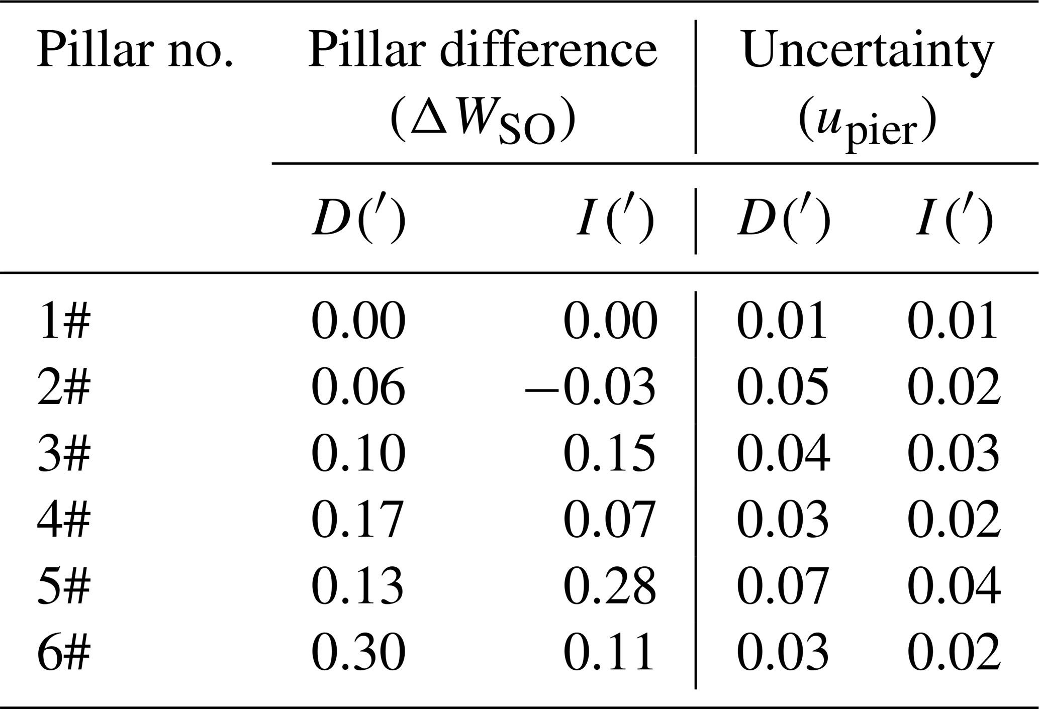
In comparison, different instruments may be installed on different observation pillars. To unify the observation results of these instruments to the standard pillar for comparison with the standard instrument's results, pillar difference corrections must be applied to the measurement data of each instrument. These pillar differences (ΔW_SO) and their uncertainty (u_pier) can be obtained from the measurement results of pillar differences at each observatories. They are obtained by using repeated measurement data and calculating according to Eq. (A6) or Eq. (A7). They can also be checked using all the comparison data.

Given that the magnetic gradient within the observation room is very small, the pillar difference is therefore typically minimal. Nevertheless, prior to initiating each comparison process, it was remeasured to ensure accuracy. Table B1 presents the pillar differences and their uncertainties at the observatory where the comparison is conduced.

Table B1 Pillar differences and their uncertainties.

B4 The total synthesized uncertainty

The total synthesized uncertainty for each instrument is then aggregated as the root sum square of all contributing factors, according to Eq. (B8):

$$\begin{array}{}\text{(B8)}& u_i=\sqrt{u_{\mathrm{inst},i}^{\mathrm{2}}+u_{\mathrm{oper}}^{\mathrm{2}}+u_{\mathrm{rep},i}^{\mathrm{2}}+u_{\mathrm{pier},i}^{\mathrm{2}}}.\end{array}$$

Finally, the ensemble mean (μ_group) and combined uncertainty (u_group) for all instruments are computed using a weighted average approach. Weights (ω_i) are assigned inversely proportional to the square of each instrument's total uncertainty, ensuring higher precision instruments exert greater influence, using Eqs. (B9) and (B10):

$$\begin{array}{}\text{(B9)}& {\displaystyle }{\mathit{\mu }}_{\mathrm{group}}={\displaystyle \frac{{\sum }_{i=\mathrm{1}}^N{\mathit{\omega }}_i{\mathit{\mu }}_i}{{\sum }_i^N{\mathit{\omega }}_i}},{\mathit{\omega }}_i={\displaystyle \frac{\mathrm{1}}{u_i^{\mathrm{2}}}},\text{(B10)}& {\displaystyle }{u}_{\mathrm{group}}={\displaystyle \frac{\mathrm{1}}{\sqrt{{\sum }_i^N{\mathit{\omega }}_i}}}.\end{array}$$

This comprehensive methodology transforms the comparison into a robust experiment integrating multi operators' collaboration, parallel instrumentation, and repeated measurements, ensuring rigorous uncertainty quantification.

B5 Multi years comparison analysis method

Building on the uncertainty analysis of single comparison sessions, this section evaluates the long term stability and robustness of the reference instrument using data accumulated over 12 comparisons within the GNC. Each comparison session involves comparing the reference instrument, mounted on a standardized pillar, against the ensemble results of participating instruments. Since the reference instrument requires no pillar correction, its mean value (μ_s) and associated uncertainty (u_rep,s) are derived from 6–8 repeated measurements per session. The repeatability standard deviation (s_rep,s) and corresponding uncertainty (u_rep,s) are calculated using Eqs. (B11) and (B12):

$$\begin{array}{}\text{(B11)}& {\displaystyle }{u}_{\mathrm{rep},\mathrm{s}}={\displaystyle \frac{s_{\mathrm{rep},\mathrm{s}}}{\sqrt{N}}},\text{(B12)}& {\displaystyle }{s}_{\mathrm{rep},\mathrm{s}}=\sqrt{{\displaystyle \frac{\mathrm{1}}{N-\mathrm{1}}}{\sum }_{k=\mathrm{1}}^N{\left(x_{\mathrm{s},k}-{\mathit{\mu }}_{\mathrm{s}}\right)}^{\mathrm{2}}},{\mathit{\mu }}_{\mathrm{s}}={\displaystyle \frac{\mathrm{1}}{N}}{\sum }_{k=\mathrm{1}}^N{x}_{\mathrm{s},k}.\end{array}$$

The total uncertainty of the reference instrument (u_s) incorporates its internal error (u_inst,s), the operator dependency uncertainty (u_oper), and repeatability uncertainty, as expressed in Eq. (B13):

$$\begin{array}{}\text{(B13)}& u_{\mathrm{s}}=\sqrt{u_{\mathrm{inst},\mathrm{s}}^{\mathrm{2}}+u_{\mathrm{oper}}^{\mathrm{2}}+u_{\mathrm{rep},\mathrm{s}}^{\mathrm{2}}}.\end{array}$$

The difference (Δ) between the reference instrument and the weighted ensemble mean (μ_group) of all participating instruments, along with its uncertainty (u_Δ), is quantified for each session using Eqs. (B14) and (B15):

$$\begin{array}{}\text{(B14)}& {\displaystyle }\mathrm{\Delta }={\mathit{\mu }}_{\mathrm{group}}-{\mathit{\mu }}_{\mathrm{s}},\text{(B15)}& {\displaystyle }{u}_{\mathrm{\Delta }}=\sqrt{u_{\mathrm{s}}^{\mathrm{2}}+u_{\mathrm{group}}^{\mathrm{2}}}.\end{array}$$

A consistency criterion (|Δ| ≤ 2u_Δ) is applied to verify agreement at a 95 % confidence level.

To assess long term stability, differences (Δ) from M years comparison sessions are compiled into a time series plot, enabling visual detection of potential drifts caused by environmental fluctuations or instrumental aging. The multi-year mean difference ($\stackrel{\mathrm{‾}}{\mathrm{\Delta }}$) and its uncertainty ($u_{\stackrel{\mathrm{‾}}{\mathrm{\Delta }}}$) are calculated through Eqs. (B16) and (B17):

$$\begin{array}{}\text{(B16)}& {\displaystyle }\stackrel{\mathrm{‾}}{\mathrm{\Delta }}={\displaystyle \frac{\mathrm{1}}{M}}{\sum }_{m=\mathrm{1}}^M{\mathrm{\Delta }}_m,\text{(B17)}& {\displaystyle }{u}_{\stackrel{\mathrm{‾}}{\mathrm{\Delta }}}=\sqrt{{\displaystyle \frac{\mathrm{1}}{M}}{\sum }_{m=\mathrm{1}}^M{u}_{\mathrm{\Delta },m}^{\mathrm{2}}+{\left({\displaystyle \frac{s_{\mathrm{\Delta }}}{\sqrt{M}}}\right)}^{\mathrm{2}}},\end{array}$$

where, (s_Δ), represents the standard deviation of Δ across all sessions. The final robustness criterion ($\left|\stackrel{\mathrm{‾}}{\mathrm{\Delta }}\right|$ ≤ $\mathrm{2}{u}_{\stackrel{\mathrm{‾}}{\mathrm{\Delta }}}$) ensures the reference instrument's performance remains within acceptable bounds over extended periods. This integrated approach combines temporal trend analysis with uncertainty propagation, providing a comprehensive evaluation framework for maintaining measurement integrity in long term geomagnetic monitoring.