THEMIS: spin axis magnetic field reconstruction

The Time History of Events and Macroscale Interactions during Substorms (THEMIS) mission investigates the coupling between the solar wind and Earth's magnetosphere using five identical spinning spacecraft. Each spacecraft rotates at a predefined rate to stabilize it and carries a suite of instruments, including a fluxgate magnetometer (FGM) that measures the three-dimensional magnetic field. Since 24 May 2024, the FGM on board THEMIS E has no longer recorded the magnetic field component along the spin axis, while the two components approximately within the spin plane remain fully available.

We present a method to reconstruct the missing magnetic field component using data from these two remaining components together with the spacecraft spin, yielding full three-component magnetic field vectors at spin period cadence and with an effective bandwidth of $\mathrm{1}/\mathrm{60}$ Hz. The approach was validated using original THEMIS E data from 2017 to 2020, when all three sensor components were available. We further estimated the reconstruction noise floor, indicating that the method is unlikely to be limited by sensor noise. These results demonstrate that on a spinning spacecraft, two components whose sensor axes lie close to, but not exactly in, the spin plane are sufficient to reconstruct three-dimensional magnetic field vectors, allowing continued magnetospheric observations despite the loss of one sensor component.

1 Introduction

Continuous and accurately calibrated magnetic field measurements are essential to study the large-scale interaction between the solar wind and Earth's magnetosphere. Magnetometers onboard spacecraft provide these observations and are therefore fundamental for investigating the coupling between interplanetary and terrestrial magnetic fields (e.g., Balogh, 2010).

The Time History of Events and Macroscale Interactions during Substorms (THEMIS) mission (Angelopoulos, 2008) is designed to study these large-scale interactions and consists of five identical spacecraft, each equipped with a fluxgate magnetometer (FGM, Auster et al., 2008). The spacecraft spin at a predefined rate denoted as T_spin (≈ 3–4 s) to stabilize them. The FGM is designed to measure low magnetic fields present in the solar wind as well as the ambient terrestrial magnetic field in close proximity to Earth in three dimensions. One of its sensitive axes is approximately aligned with the spin axis (hereafter referred to as the spin axis sensor), while the other two are nearly aligned with the spin plane (hereafter referred to as spin plane sensors), although they deviate slightly from the exact spin plane orientation. The three sensors are nearly, but not perfectly, orthogonally aligned. These deviations occur because there are no instrument alignment requirements for the mission (Auster et al., 2008), and the spin axis, and thus the spin plane, changes over the course of the mission.

Figure 1 Sketch of coordinate systems: (a) actual sensor axes (in red), orthogonalized sensor axes (in blue), (b) spin axis (in black) and rotation angles ${\mathit{\sigma }}_{P_x}$ and ${\mathit{\sigma }}_{P_y}$ in the sensor package system. Panel (c) illustrates the angles α_S1 and α_S2 between the spin axis and the spin plan sensor S1 and S2. For simplicity, the angle α_S3 between the spin axis sensor S3 and the spin axis is not shown. Images adapted and modified from Plaschke et al. (2019) in courtesy of F. Plaschke.

Careful calibration of the FGM data is required to convert the raw magnetometer output B_S into physically meaningful magnetic field measurements B (see e.g., Auster et al., 2008; Frühauff et al., 2017; Plaschke et al., 2019). B_S is recorded in the non-orthogonal sensor coordinate system that co-rotates with the spacecraft. The complete transformation into B involves several procedures: (1) applying gain factors that convert the raw instrument output into physical units, specific to each sensor axis; (2) geometrically transforming the measurements from the non-orthogonal sensor coordinate system into an orthogonal, spin axis aligned coordinate system; and (3) subtracting offsets, which represent non-vanishing outputs of the magnetometer in the absence of ambient fields, originating from the instruments themselves and from spacecraft-generated stray fields. This transformation can be expressed as:

$$\begin{array}{}\text{(1)}& \mathit{B}=\mathbf{C}\cdot ({\mathit{B}}_{\mathrm{S}}-{\mathit{O}}_{\mathrm{S}}),\end{array}$$

where O_S denotes the offset vector and C the coupling matrix, which depends on three gain factors and six orientation angles of the sensor axes. Of these, three describe the internal sensor geometry, while the remaining three define the alignment between the sensor and spacecraft coordinate systems (for details, see Sect. 2.1).

Recently, the THEMIS E spacecraft (THE) has encountered some challenges, particularly due to radiation damage to the instrument's Analog-to-Digital Converter (ADC). Notably, since 24 May 2024, at 22:54:06 UTC, no magnetic field measurements have been obtained from the spin axis sensor. In contrast, the two remaining spin plane sensors continue to operate nominally.

Because the two remaining sensor axes are slightly inclined relative to the spin plane, the missing spin axis component can be reconstructed from their measurements. In the non-orthogonal sensor coordinate system, which co-rotates with the spacecraft, the magnetic field projected onto each spin plane sensor varies periodically as the spacecraft spins. A magnetic field component within the spin plane therefore appears as a sinusoidal signal, while a constant magnetic field component along the spin axis manifests as a constant contribution in the time series. This projected spin axis contribution B_pSA is indistinguishable from the result of a true instrumental offset in the same, co-rotating coordinate system. Therefore, accurately determining the spin plane offsets is crucial for reconstructing the spin axis signal.

Assuming that the spin plane offsets have been accurately estimated, the magnitude of the magnetic field component along the spin axis, B_SA, projected onto the axes of sensors S1 and S2, can be expressed as

$$\begin{array}{}\text{(2)}& B_{\text{pSA}}=B_{\text{SA}}\cdot \cos \mathit{\alpha },\end{array}$$

where α (α_S1 or α_S2) is the angle between the axis of the respective sensor and the spin axis (see Fig. 1c).

In this paper, we present a method to calculate the projected spin axis contribution and subsequently recover the missing spin axis magnetic field component. We begin by formulating the mathematical basis of the problem, followed by a description of its implementation in the updated calibration process. Finally, we compare the recovered data against measurements from 2017 to 2020, when all sensor axes were fully operational. The three year time span was chosen as a trade-off between instrument degradation, temporal proximity to the current mission phase, and capturing variations in the calibration parameters, thereby allowing us to verify the recovery under different conditions (for details, see Sect. 2.1). The approach restores the full vector magnetic field at spin period resolution and thereby extends the THEMIS FGM dataset as a continuous resource for magnetospheric research.

2 Mathematical Background

The mathematical approach to the problem consists of two parts. The first is the geometric transformation of the non-orthogonal system associated with the instrument into an orthogonal system that is related to the reference frame of the spinning spacecraft. It is realized in several steps, while here we are only interested in the directional nature of the measured output in order to obtain the angles between the sensors and the spin axis. The second part is devoted to the conversion of the two available sensor outputs into plausible records of the magnetic field in the respective directions. Taking into account the fact that the magnetic field oriented along the spin axis persistently contributes to these results, it is possible to separate this component and determine it with sufficient accuracy.

The orientation of the three non-orthogonal sensor axes, S1, S2 and S3, is illustrated in red in Fig. 1a. The raw magnetometer output along these axes is transformed into an orthogonal spin axis-aligned coordinate system (x,y and z) with physical meaningful units using the coupling matrix C (see Eq. 1). The coupling matrix can be expressed as

$$\begin{array}{}\text{(3)}& \mathbf{C}=\mathbf{\Phi }\cdot \mathbf{\Sigma }\cdot \mathbf{\Gamma }\cdot \mathbf{G},\end{array}$$

where each submatrix accounts for a specific step in the coordinate transformation. We first introduce the coordinate systems and derive an expression for α, before describing the determination of B_pSA from the spin plane measurements.

2.1 Coordinate System and Transformation Matrices

To clarify the geometry of the problem, we follow the formalism introduced by Plaschke et al. (2019), which builds on Kepko et al. (1996). We adopt their notation for consistency, while noting that the final implementation of our coupling matrix C differs slightly in form while yielding identical results. The conversion matrix Γ transforms from the non-orthogonal sensor axes coordinate system (red axes in Fig. 1a) into an orthogonal sensor package coordinate system (P_x, P_y and P_z), represented by the blue axes in Fig. 1. With ${\widehat{\mathit{p}}}_j$ denoting the unit vector along P_j, this can be written as Eqs. (4)–(6):

$$\begin{array}{}\text{(4)}& {\displaystyle }\text{S1}=\sin {\mathit{\theta }}_{\text{S1}}{\widehat{\mathit{p}}}_x+\cos {\mathit{\theta }}_{\text{S1}}{\widehat{\mathit{p}}}_z,\text{(5)}& {\displaystyle }\mathrm{\text{S2}}=\cos {\mathit{\varphi }}_{\text{S12}}\sin {\mathit{\theta }}_{\text{S2}}{\widehat{\mathit{p}}}_x+\sin {\mathit{\varphi }}_{\text{S12}}\sin {\mathit{\theta }}_{\text{S2}}{\widehat{\mathit{p}}}_y+\cos {\mathit{\theta }}_{\text{S2}}{\widehat{\mathit{p}}}_z,\text{(6)}& {\displaystyle }\text{S3}={\widehat{\mathit{p}}}_z,\end{array}$$

and thus

$$\begin{array}{}\text{(7)}& \mathbf{\Gamma }={\left(\begin{array}{ccc}\sin {\mathit{\theta }}_{\text{S1}}& \mathrm{0}& \cos {\mathit{\theta }}_{\text{S1}}\\ \cos {\mathit{\varphi }}_{\text{S12}}\sin {\mathit{\theta }}_{\text{S2}}& \sin {\mathit{\varphi }}_{\text{S12}}\sin {\mathit{\theta }}_{\text{S2}}& \cos {\mathit{\theta }}_{\text{S2}}\\ \mathrm{0}& \mathrm{0}& \mathrm{1}\end{array}\right)}^{-\mathrm{1}}.\end{array}$$

The angles θ_S1, θ_S2, and ϕ_S12 define the internal geometry of the sensor axes (see Fig. 1a). The subsequent rotation matrix Σ aligns the sensor-package system with the spacecraft spin axis which is represented in black in Fig. 1b:

$$\begin{array}{}\text{(8)}& \mathbf{\Sigma }=\left(\begin{array}{ccc}\cos {\mathit{\sigma }}_{P_x}& \mathrm{0}& -\sin {\mathit{\sigma }}_{P_x}\\ \mathrm{0}& \mathrm{1}& \mathrm{0}\\ \sin {\mathit{\sigma }}_{P_x}& \mathrm{0}& \cos {\mathit{\sigma }}_{P_x}\end{array}\right)\times \left(\begin{array}{ccc}\mathrm{1}& \mathrm{0}& \mathrm{0}\\ \mathrm{0}& \cos {\mathit{\sigma }}_{P_y}& -\sin {\mathit{\sigma }}_{P_y}\\ \mathrm{0}& \sin {\mathit{\sigma }}_{P_y}& \cos {\mathit{\sigma }}_{P_y}\end{array}\right),\end{array}$$

where ${\mathit{\sigma }}_{P_x}$ and ${\mathit{\sigma }}_{P_y}$ describe the tilt of the spin axis relative to the sensor package coordinate system (see Fig. 1b). Finally, the azimuthal rotation around the spin axis by the angle ϕ_a (not shown in Fig. 1) is represented by

$$\begin{array}{}\text{(9)}& \mathbf{\Phi }=\left(\begin{array}{ccc}\cos {\mathit{\varphi }}_{\mathrm{a}}& -\sin {\mathit{\varphi }}_{\mathrm{a}}& \mathrm{0}\\ \sin {\mathit{\varphi }}_{\mathrm{a}}& \cos {\mathit{\varphi }}_{\mathrm{a}}& \mathrm{0}\\ \mathrm{0}& \mathrm{0}& \mathrm{1}\end{array}\right).\end{array}$$

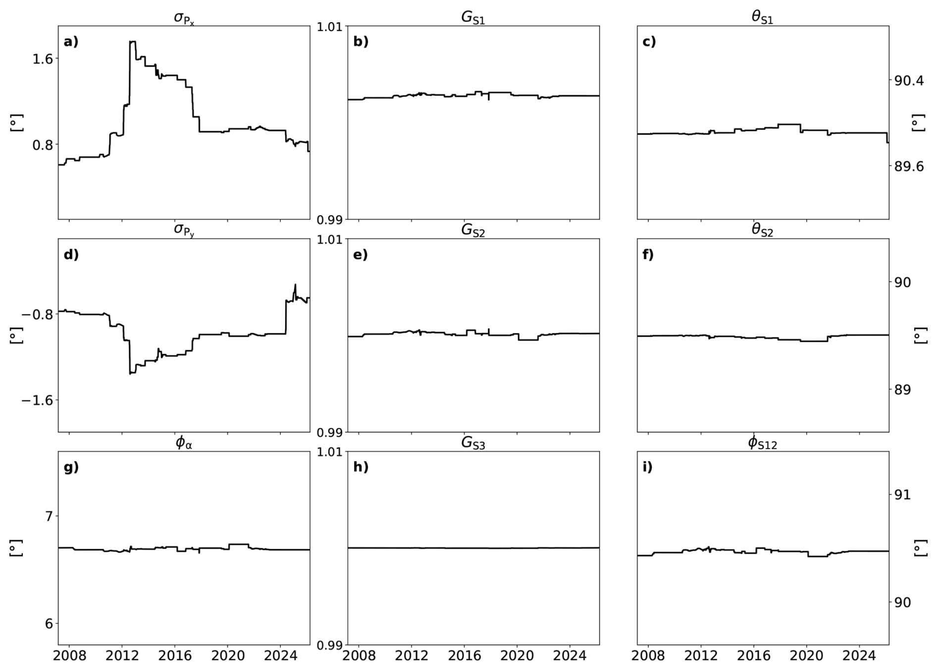
The rotation around the spin axis arises from the mounting orientation of the FGM on the spacecraft. The angle ϕ_a is required to transform the measurements from the sensor coordinate system into a physically meaningful spacecraft-fixed coordinate system, from which further transformations into other coordinate systems, such as geocentric systems, can be performed. Although not required for the subsequent analysis, this rotation is included here to complete the description of the coordinate transformation. In Fig. 2 we show the evolution of the calibration parameters over the course of the mission. Whereas $\mathbf{\Gamma }({\mathit{\theta }}_{\text{S1}},{\mathit{\theta }}_{\text{S2}},{\mathit{\varphi }}_{\text{S12}})$ remains nearly constant throughout the mission for a well-constructed magnetometer as can be seen in Fig. 2c, f, and i, $\mathbf{\Sigma }({\mathit{\sigma }}_{P_x},{\mathit{\sigma }}_{P_y})$ can vary over time due to spacecraft maneuvers and gravity gradients that alter the moment of inertia and thereby the spin axis orientation. This is present in Fig. 2a and d (for more details on the coupling matrix see Plaschke et al., 2019).

Figure 2 Evolution of calibration parameter: ${\mathit{\sigma }}_{P_x}$, ${\mathit{\sigma }}_{P_y}$, and ϕ_α are the rotation angles around the orthogonalized sensor axes (c.f. with blue coordinate system Fig. 1). G_S1, G_S2, and G_S3 are the gains along the sensor axes. θ_S1, θ_S2, and ϕ_S12 are the internal sensor angles.

2.2 Determination of the Sensor-to-Spin-Axis Angles

The angles α_S1, α_S2, and α_S3 (see Fig. 1c) can be obtained from the projection of the spin axis onto the sensor axes using the geometric definition of the scalar product of two vectors, $\cos \mathit{\theta }=\mathit{u}\cdot \mathit{v}/\left(\right|\mathit{u}|\cdot |\mathit{v}\left|\right)$. In the orthogonal spin axis-aligned coordinate system, the spin axis unit vector is given by $\mathit{z}=[\mathrm{0},\mathrm{0},\mathrm{1}{]}^{\mathrm{T}}$. Using the transformation matrices, the calculation of the angles can be expressed as:

$$\begin{array}{}\text{(10)}& \begin{array}{rl}\left(\begin{array}{c}{\mathit{\alpha }}_{\text{S1}}\\ {\mathit{\alpha }}_{\text{S2}}\\ {\mathit{\alpha }}_{\text{S3}}\end{array}\right)=& {\cos }^{-\mathrm{1}}\left({\mathbf{\Gamma }}^{-\mathrm{1}}\cdot {\mathbf{\Sigma }}^{-\mathrm{1}}\cdot {\mathbf{\Phi }}^{-\mathrm{1}}\cdot \mathit{z}\right)\\ =& {\cos }^{-\mathrm{1}}\left(\begin{array}{c}\sin {\mathit{\theta }}_{\text{S1}}\sin {\mathit{\sigma }}_{P_x}+\cos {\mathit{\theta }}_{\text{S1}}\cos {\mathit{\sigma }}_{P_x}\cos {\mathit{\sigma }}_{P_y}\\ \begin{array}{c}\cos {\mathit{\varphi }}_{\text{S12}}\sin {\mathit{\theta }}_{\text{S2}}\sin {\mathit{\sigma }}_{P_x}\\ +\sin {\mathit{\varphi }}_{\text{S12}}\sin {\mathit{\theta }}_{\text{S2}}\cos {\mathit{\sigma }}_{P_x}\sin {\mathit{\sigma }}_{P_y}\\ +\cos {\mathit{\theta }}_{\text{S2}}\cos {\mathit{\sigma }}_{P_x}\cos {\mathit{\sigma }}_{P_y}\end{array}\\ \cos {\mathit{\sigma }}_{P_x}\cos {\mathit{\sigma }}_{P_y}\end{array}\right).\end{array}\end{array}$$

Assuming that θ_S1, θ_S2, and ϕ_S12 remain constant (cf. Fig. 2), the parameters ${\mathit{\sigma }}_{P_x}$ and ${\mathit{\sigma }}_{P_y}$ can be derived from Eq. (10) using independently known values of α_S1, α_S2, and α_S3 (see Sect. 3 for details).

2.3 Gain Matrix and Determination of the Projected Spin Axis Contribution

The gain matrix G applies the sensor-specific conversion factors into meaningful physical units:

$$\begin{array}{}\text{(11)}& \mathbf{G}=\left(\begin{array}{ccc}g{G}_{\mathrm{p}}& \mathrm{0}& \mathrm{0}\\ \mathrm{0}& G_{\mathrm{p}}/g& \mathrm{0}\\ \mathrm{0}& \mathrm{0}& G_{\mathrm{a}}\end{array}\right),\end{array}$$

where g is the ratio of the spin plane gains $G_{\text{S1}}/G_{\text{S2}}$, and $G_{\mathrm{p}}(=\sqrt{G_{\text{S1}}{G}_{\text{S2}}})$ and G_a are the absolute gains for the spin plane and the spin axis sensors, respectively (Plaschke et al., 2019). To determine the projected spin axis contribution B_pSA from the measurements of the spin plane sensor axes data B_S1 and B_S2, we first subtract the offset vector O_S and converting to physical units by applying the corresponding gain factors. The conversion to the modified raw data B_raw is calculated by:

$$\begin{array}{}\text{(12)}& {\displaystyle }{B}_{\text{raw},\mathrm{1}}=gG\mathrm{p}(B_{\text{S1}}-O_{\text{S1}}),\text{(13)}& {\displaystyle }{B}_{\text{raw},\mathrm{2}}={\displaystyle \frac{G_{\mathrm{p}}}{g}}(B_{\text{S2}}-O_{\text{S2}}).\end{array}$$

Subsequently, we apply a low-pass Butterworth filter (e.g. Thompson, 2014) to B_raw,1 and B_raw,2 in order to suppress high-frequency variations while preserving the spin modulated signal. The filter is applied twice, once forward and once backwards, using a second-order filter with a cutoff frequency of f_cut=2ω_s, with ${\mathit{\omega }}_{\mathrm{s}}=\mathrm{2}\mathit{\pi }/T_{\text{spin}}$ denoting the angular spin frequency. This results in the low-pass filtered data B_lp,1 and B_lp,2. The resulting filter has zero phase and an effective order of four (e.g. Gustafsson, 1996). The low-pass filtered data are then fitted independently with a least-squares fit. The corresponding fitting function is given by:

$$\begin{array}{}\text{(14)}& \begin{array}{rl}{B}_{\text{fit}}\left(\mathit{\tau }\right)& =\underset{B_{\text{spinplane}}}{\underbrace{(A+B\cdot \mathit{\tau })\cdot \cos ({\mathit{\omega }}_{\mathrm{s}}\cdot \mathit{\tau }-\mathit{\phi })}}+\underset{B_{\text{pSA}}}{\underbrace{C+D\cdot \mathit{\tau }}}\\ & =B_{\text{spinplane}}\left(\mathit{\tau }\right)+B_{\text{pSA}}\left(\mathit{\tau }\right).\end{array}\end{array}$$

Here, τ denotes the time within the fitting window. The term $(A+B\cdot \mathit{\tau })$ represents the linearly time-varying amplitude of the sinusoidal component of the fit, φ is the phase shift due to the projection of the magnetic field onto the spin plane, and the term $C+D\cdot \mathit{\tau }$ is the residual, time-varying offset. Accordingly, the first term $(A+B\cdot \mathit{\tau })\cdot \cos ({\mathit{\omega }}_{\mathrm{s}}\cdot (\mathit{\tau }-\mathit{\phi }\left)\right)$ corresponds to the measurement of the spin plane magnetic field in the direction of the spin plane sensor axis (B_spinplane), whereas the second term $C+D\cdot \mathit{\tau }$ represents the projected spin axis contribution (B_pSA). The parameters A, B, C, D and φ are free fitting parameters and may differ between the two components, while T_spin, and thus ω_s, is provided by the state file of THE and is the same for both fits. This approach allows us to distinguish between the spin‐modulated variation within the spin plane and the slowly varying spin axis contribution.

Figure 3 Flow chart illustrating the recovery of the spin axis measurements. The small boxes below each step show which variables are determined. The details of the individual steps are explained in the text.

3 Implementation

In this section, we describe the procedure used to recover the missing sensor measurement along the spin axis. The overall workflow is summarized in the flow chart shown in Fig. 3, with each step and its derived variables explained in the subsequent sections.

3.1 Determination of the Projected Spin Axis Contribution

We utilize the low-telemetry channel (FGL) of the FGM (for details on the instrument and data products, see Auster et al., 2008), which provides vector magnetic field data with sampling rates between 4 and 128 Hz. Since 27 July 2015, the FGL sampling rate on THE has been f_FGL = 16 Hz. This sampling rate yields several tens of samples per spin and is therefore sufficient to resolve the spin modulation required for our fitting procedure. We do not use the high-telemetry channel (FGH at 128 Hz), as it is rarely available nor the onboard spin resolution product (FGS, one vector per spin), because its resampling removes the spin modulation required for the fit.

We start with B_raw,1 and B_raw,2 as obtained from Eqs. (12) and (13). We then apply the low-pass filter to each component, yielding the low-pass filtered data B_lp,1 and B_lp,2. Finally, we fit the spin plane sensor components of B_lp using Eq. (14) with a sliding window of 2.5 spin periods, shifted by one spin period between consecutive fits. Accordingly, τ ranges from 0 to 2.5 T_spin. We require the number of samples per fit window to be between 90 % and 110 % of the expected number,$f_{\text{FGL}}\cdot \mathrm{2.5}\cdot T_{\text{spin}}$, in order to reject windows affected by data gaps. This results in a slightly variable number of samples per window. In contrast, using a fixed number of samples would lead to windows that do not exactly cover the intended 2.5 spin periods. A comparison of both approaches (not shown) exhibits only negligible differences in the final recovered values.

As a measure of the fit uncertainty, we compute the mean squared difference between B_fit and B_lp for each window:

$$\begin{array}{}\text{(15)}& f_{\text{min}}={\displaystyle \frac{\mathrm{1}}{n}}\sum _{j=\mathrm{1}}^n\left(B_{\text{fit}}\right({\mathit{\tau }}_j)-B_{\text{lp}}({\mathit{\tau }}_j){)}^{\mathrm{2}}.\end{array}$$

Here, n denotes the number of measurement points per window. The quantity f_min contains everything not explained by the fit, including remaining higher-frequency contributions, sensor noise, and low-frequency variations that are not captured by the model. While the latter is the uncertainty we aim to quantify, the other contributions also affect the fit quality and must therefore be taken into account.

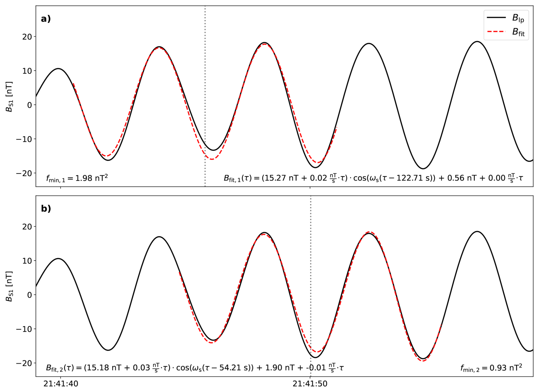
Figure 4 Two consecutive fits applied to THE B_lp (black) to calculate B_pSA on 23 July 2017. The dashed red lines represent the applied fit B_fit and are only shown over the corresponding fit intervals. The fit in panel (b) is shifted by one spin period relative to the fit in panel (a). In addition, at the bottom of both panels, the corresponding f_min value and fitting parameters for each fit are given.

Each fit window yields a time-dependent estimate B_pSA(τ). We evaluate B_pSA(τ) at the window center, $\mathit{\tau }=\mathrm{1.25}\cdot T_{\text{spin}}$, to obtain one estimate B_pSA(t_c) per window centered at time t_c. This yields a time series of the projected spin axis contribution B_pSA at spin resolution (≈ 3–4 s). An example of the fitting process for two consecutive fits to B_lp,1 is shown in Fig. 4. In Fig. 4a, the fit window is centered at 21:41:46 UTC on 23 July 2017; in Fig. 4b, the window is shifted by T_spin and centered at 21:41:50 UTC.

We calculate the projected spin axis contribution B_pSA independently for both spin plane component. From these two estimates, we use the result from the sensor that is more closely aligned with the spin axis, i.e., the one axis for which $|\mathrm{90}\mathit{°}-{\mathit{\alpha }}_{\text{S1},\text{S2}}|$ is larger. For this sensor, the projection of the spin axis component is more pronounced.

To suppress the influence of poor fits, we calculate a weighted moving average with a window length L of 1 min:

$$\begin{array}{}\text{(16)}& B_{\text{wma}}\left(t\right)={\displaystyle \frac{{\sum }_{j:|t_j-t|\le L/\mathrm{2}}{B}_{\text{pSA}}\left(t_j\right)\cdot w(t_j,t)}{{\sum }_{j:|t_j-t|\le L/\mathrm{2}}w(t_j,t)}},\end{array}$$

where the weight is defined as

$$\begin{array}{}\text{(17)}& w(t_j,t)=w_{\text{fit}}\left(t_j\right)\cdot w_{\mathrm{t}}(t_j,t),\end{array}$$

with the fitting weight

$$\begin{array}{}\text{(18)}& w_{\text{fit}}\left(t_j\right)={\displaystyle \frac{\mathrm{1}}{f_{\text{min}}\left(t_j\right)}}\end{array}$$

and the time-distance weight

$$\begin{array}{}\text{(19)}& w_{\mathrm{t}}(t_j,t)=\left\{\begin{array}{ll}\mathrm{1}-{\displaystyle \frac{|t_j-t|}{L/\mathrm{2}}},& |t_j-t|\le \frac{L}{\mathrm{2}},\\ \mathrm{0},& \text{otherwise.}\end{array}\right.\end{array}$$

The fitting weight w_fit reduces the influence of poorly fitted windows, whereas the triangular time–distance weight w_t emphasizes samples near the center of the averaging interval. The weighted moving average B_wma(t) is the final estimate of the projected spin axis contribution and provides an effective bandwidth of $\mathrm{1}/L=\mathrm{1}/\mathrm{60}$ Hz.

3.2 Recovery of the Spin Axis Component

Having obtained the weighted moving average of the projected spin axis contribution B_wma, we reconstruct the missing spin axis measurement B_r by dividing B_wma by the factor cos α. This requires accurate knowledge of the angle α between a spin plane sensor and the spin axis (see Fig. 1c). As discussed in Sect. 2.2, these angles could in principle be derived from the coupling matrix C (see Eq. 10). However, due to the loss of the spin axis measurement, a direct in-flight calibration of C is no longer feasible. This is because the regular calibration process can no longer uniquely distinguish whether a constant offset in the raw data originates from the true spin axis signal, from remaining spin plane offsets, or from inaccuracies in the angular terms of C.

To estimate the angles α_S1 and α_S2, we therefore use Eq. (2) in combination with the fitted B_pSA and a modeled magnetic field approximation for the spin axis component B_SA. The angle determination is restricted to perigee intervals, where the high magnetic field strength ensures that small perturbations have only a minor relative impact on the derived angles, as any residual sensor offsets and their uncertainties become negligible in comparison. We define the perigee region by a minimum field strength of 10 000 nT.

As model field B_SA we use the International Geomagnetic Reference Field (IGRF) superposed with the model field of Tsyganenko (1989), hereafter referred to as T89. The IGRF, which represents the internal part of the Earth's magnetic field, is a good approximation of the actual terrestrial magnetic field near perigee (e.g.  Alken et al., 2021), while the T89 model provides a simple and widely used empirical description of the external magnetospheric field, parameterized by the geomagnetic k_p index (Matzka et al., 2021).

Using Eq. (2), the comparison between B_pSA and B_SA yields updated estimates of α_S1 and α_S2. To evaluate the validity of this approach, we compared the estimated α values with those from the calibration matrix over a 3-year period from 2017 to 2020. The angles differ only minimally, with median deviations of Δα_S1 = 0.045° and Δα_S2 = 0.058°.

Since May 2024, the angles between the spin axis and the two sensor axes have been 89.82° for α_S1 and 90.92° for α_S2; the corresponding interquartile ranges are 89.81 to 89.84° for α_S1 and 90.91 to 90.93° for α_S2. The orientation of the spin axis changes over time due to gravity-gradient effects and orbital maneuvers. As a result, the effective coupling matrix also varies with time, making continuous updates of these parameters necessary. The updated estimates of α_S1 and α_S2 are used in a least-squares optimization of the parameters ${\mathit{\sigma }}_{P_x}$ and ${\mathit{\sigma }}_{P_y}$, ensuring continued calibration of the coupling matrix C throughout the mission. For this purpose, we use the first two components of Eq. (10) together with the updated values of α_S1 and α_S2, while treating all calibration file entries other than ${\mathit{\sigma }}_{P_x}$ and ${\mathit{\sigma }}_{P_y}$ as fixed. Each angle estimate thus provides two constraints on the two unknown parameters, and all available estimates are combined into an overdetermined system that is solved by least squares.

As discussed in Appendix A, additional efforts were made to further refine and improve the recovered spin axis signal. However, the analysis reveals that such attempts not only proved challenging but also led to inconsistent results. Therefore, we consider B_r as the final data product used to replace the missing spin axis measurement. It should be noted that deviations between the original measurements and the recovered signal remain, which are analyzed and discussed in the following sections.

4 Comparison of Results

To validate the accuracy of the recovery method, we compare the recovered magnetic field component with original measurements from THE over a 3-year time span from 2017 to 2020, and with data from THA as reference spacecraft for periods after the loss of the spin axis sensor component measurements (since May 2024).

Figure 5 Comparison between recovered (B_r, red), original (B_FGS, black), and model (B_T89, blue) magnetic field data for (a) a magnetospheric interval and (b) a magnetosheath interval following multiple magnetopause crossings (vertical gray lines) in 2017. The original data correspond to calibrated FGS measurements from THE; the original data were additionally smoothed using a weighted moving average with time-distance scaling and a window length of 1 min. Panels (c) and (d) show enlarged views of the intervals 07:00–08:00 UTC from panel (a) and 13:30–14:30 UTC from panel (b), respectively.

4.1 Qualitative Comparison

In Fig. 5 we present two representative qualitative comparisons from 2017: one interval in the magnetosphere from 24 April (Fig. 5a), together with a more detailed view from 07:00–08:00 UTC (Fig. 5c); one interval from 29 July in the magnetosheath including multiple magnetopause crossings (Fig. 5b) with a 1 h zoom from 13:30–14:30 UTC (Fig. 5d).

In all panels, the original measurement B_FGS, recovered data B_r, and model field B_T89 are shown in black, red, and blue, respectively. To ensure a consistent comparison with B_r, we also apply a weighted moving average with time-distance scaling and a window length of 1 min to B_FGS. In Fig. 5a, the recovered data closely follow the original measurements, with minor differences arising at the beginning of the shown interval. Figure 5b presents data where THE traversed the magnetopause multiple times between 12:24 and 15:48 UTC. Magnetopause crossings, identified using the list from Grimmich et al. (2023), are indicated by vertical gray lines. The recovered data also generally follow the original measurements, though larger deviations are observed during boundary crossings and within the magnetosheath, where the magnetic field changes rapidly. In particular, Fig. 5d shows pronounced over- and undershoots, which likely indicate limitations of the fitting approach under rapidly varying conditions. Notably, in both examples B_r provides a far better representation of the observed field than the model field B_T89, which remains valid only within the magnetosphere.

Figure 6 Comparison between recovered (B_r, red), reference spacecraft (B_FGS, black), and model (B_T89, blue) magnetic field data in (a) the magnetosheath before a magnetopause crossing at 01:49 UTC (vertical gray line) and (b) the magnetosphere in 2024. The reference data correspond to calibrated FGS measurements from THA and were additionally smoothed using a weighted moving average with time-distance scaling and a window length of 1 min. Panels (c) and (d) show enlarged views of the intervals 01:00–02:00 UTC from panel (a) and 04:00–05:00 UTC from panel (b), respectively.

Following the validation with original 2017 measurements, we next evaluate the recovery after the spin axis component became unavailable in May 2024 by comparing the recovered data B_r with simultaneous observations from the nearby reference spacecraft THA. Two representative intervals are shown in Fig. 6: magnetosheath observations prior to a magnetopause crossing from 8–9 June 2024 (Fig. 6a) and magnetosphere observations from 28–29 November 2024 (Fig. 6b). Enlarged views of these intervals are shown in Fig. 6c for 01:00–02:00 UTC and in Fig. 6d for 04:00–05:00 UTC.

In all panels, the reference measurements from THA B_FGS, B_r, and B_T89 are displayed in black, red, and blue, respectively. For consistency with the temporal resolution of the recovered data B_r, the THA reference measurements were also smoothed using a weighted moving average with time-distance scaling and a 1 min window. The recovered data are generally consistent with the reference measurements in both intervals, although enhanced deviations occur near the magnetopause and within the turbulent magnetosheath (Fig. 6a and c). In particular, Fig. 6c again highlights the larger differences in the magnetosheath. In the magnetosphere interval (Fig. 6b), discrepancies are visible between 02:45–03:30 and 06:00–08:30 UTC, which may reflect spatial separation between THE and THA (≈ 1 R_E). Without the original spin axis measurements from THE, this cannot be verified. In both examples, within the magnetosphere the recovered data provide a substantially better representation of the observed reference field than the model B_T89.

4.2 Quantitative Comparison

The examples suggest that the accuracy of the recovery depends on the spacecraft's plasma environment. To quantify this dependence, we assess the performance of the recovery method in different regions of near-Earth space. Specifically, we divide the data from 2017 to 2020 into the following regions: the magnetosphere, the magnetopause, the magnetosheath, and the solar wind. The solar wind is further subdivided into quasi-parallel and quasi-perpendicular regions upstream of the bow shock. Within the magnetosphere, we distinguish between low ($\left|B_{\text{FGS}}\right|$ < 50 nT) and high field (B_FGS > 50 nT) intervals.

To identify the different regions, we use the results from Edmond et al. (2024) who applied a combination of unsupervised machine learning methods to classify THEMIS observations into magnetosphere, magnetosheath, and solar wind observations. We make use of their publicly available dataset for THE, in which each data point is assigned to one of these regions. Magnetopause and bow shock crossings are identified by changes in the region label. In addition, to further divide the dataset, we also use magnetic field data from the FGM (fully operational in 2017 to 2020) and the omni directional ion energy flux E_flux (ESA,  McFadden et al., 2008).

Magnetospheric data are separated into low- and high-field intervals to avoid biasing the statistics, as larger absolute deviations are expected close to perigee where the magnetic field is strongest. We define the low field magnetosphere by data points that fulfill $\left|B_{\text{FGS}}\right|$ < 50 nT and are labeled as magnetosphere. Data points in the magnetosphere for which 50 nT < B_FGS are applicable belong to the high field magnetosphere. Data within ± 15 min of each magnetopause crossing are attributed to the magnetopause region. The magnetosheath is defined by the machine learning labels, except for the points near the magnetopause crossings. The solar wind dataset is used as specified by the model and then divided into quasi-parallel and quasi-perpendicular by having E_flux at 10 keV higher and lower than 20 000 ${\mathrm{cm}}^{-\mathrm{2}}{\mathrm{s}}^{-\mathrm{1}}{\mathrm{sr}}^{-\mathrm{1}}$, respectively. Manual inspection confirmed the robustness of these assignments, with few outliers that were removed from the subsets.

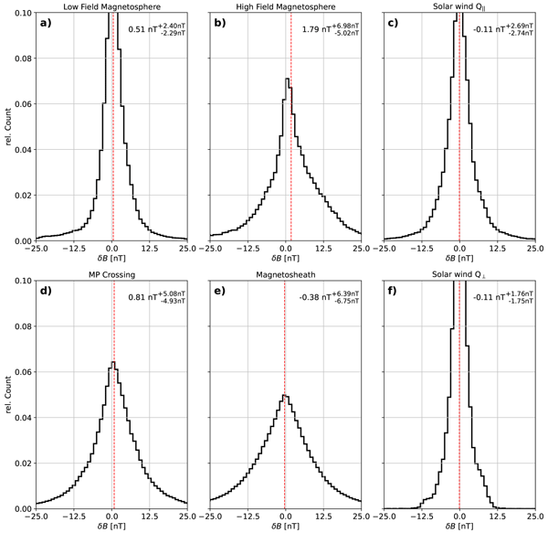
We observe 6 754 802 and 1 994 568 data points in the low and high field magnetosphere, 641 029 data points around the magnetopause, and 2 077 719 in the magnetosheath, respectively. In the solar wind, however, we observe 250 187 and 182 847 data points in the quasi-parallel and quasi-perpendicular regions, respectively. The large differences in the data quantities can be attributed to the orbital configuration of the THEMIS mission. For each region, we calculate the difference between the recovered B_r and the original spin axis measurements B_FGS:

$$\begin{array}{}\text{(20)}& \mathit{\delta }B=B_{\mathrm{r}}-B_{\text{FGS}}.\end{array}$$

As in the qualitative comparison, B_FGS was additionally smoothed using time-distance scaling and a 1 min window. The distributions of δB for the different regions are shown in Fig. 7.

Figure 7 Histograms of the deviation δB between recovered (B_r) and original (B_FGS) spin axis measurements in six different regions for a three year time span from 2017 to 2020: (a) low-field magnetosphere near perigee, (b) high-field magnetosphere, (c) quasi-parallel solar wind, (d) magnetopause crossings, (e) magnetosheath, and (f) quasi-perpendicular solar wind. The vertical red dashed lines indicate the median values, and the ± values correspond with the 25th and 75th percentiles. The calibrated FGS measurements from THE B_FGS were additionally smoothed using a weighted moving average with time-distance scaling and a window length of 1 min.

Figure 7a shows δB for the low-field magnetosphere. The distribution is nearly centered around zero, with a slight positive shift and a median value below 1 nT. In the high-field magnetosphere (Fig. 7b), the distribution is broader and also shifted to positive values, with a median value below 2 nT. Near the magnetopause (Fig. 7d) and in the magnetosheath (Fig. 7e), the distributions are comparable in shape to the high-field magnetosphere and exhibit median values, below 1 nT and below 0.5 nT, respectively. In the solar wind, both the quasi-parallel and quasi-perpendicular cases (Fig. 7c and f) show narrow distributions centered near zero, with median values below 0.5 nT.

The position of the median reflects the quality of the spin plane offset determination, with correctly chosen offsets resulting in median values close to zero. The width of the distributions, in contrast, reflects the quality of the fit and of the recovery method, with broader distributions indicating poorer performance. Larger deviations between the recovered and original measurements occur in the high-field magnetosphere, as reflected by the larger interquartile range (> 10 nT). This is expected since absolute differences become more pronounced at higher field strengths, where small relative calibration errors or filter effects can lead to larger absolute deviations.

The smallest absolute deviations are observed in the solar wind with interquartile ranges < 6 nT. The slightly larger deviations in the quasi-parallel case can be attributed to the enhanced turbulence and wave activity in the foreshock region, which complicate the fitting process (see Sect. 5). The distributions in the magnetosheath and around magnetopause crossing, however, are markedly broader. Their interquartile ranges are comparable to those of the high-field magnetosphere (> 10 nT), even though the magnetic fields themselves are much weaker. These two broader distributions can be explained due to faster changes and higher fluctuation levels in the magnetic field, which likewise complicate the fitting process there.

A somewhat different picture emerges when considering relative deviations. Using the absolute relative deviation, $\left|\mathit{\delta }B\right|/\left|B_{\text{FGS}}\right|$, we find only small relative errors in the high-field magnetosphere, with a median value of 5 %. Moderate relative deviations occur in the low-field magnetosphere and near magnetopause crossings, both with median values of about 23 %. In contrast, substantially larger median values are found in the magnetosheath and the solar wind, where they reach 80 % and 115 %, respectively. This mainly reflects the smaller magnetic field strengths in these regions, for which even small absolute residuals correspond to large relative deviations; in the magnetosheath, enhanced fluctuations further increase this effect. Consequently, when the recovered spin axis field is close to zero in the solar wind, even its sign should be interpreted with caution.

To place the differences δB in the context of the intrinsic sensor noise, we estimate a lower bound for the expected reconstruction uncertainty. Following standard random-signal theory (e.g. Bendat and Piersol, 2010), the variance of filtered stationary noise is given by

$$\begin{array}{}\text{(21)}& {\mathit{\sigma }}^{\mathrm{2}}=\underset{\mathrm{0}}{\overset{\mathrm{\infty }}{\int }}\left|H\right(f){|}^{\mathrm{2}}{\left(S_B^{\mathrm{1}/\mathrm{2}}\left(f\right)\right)}^{\mathrm{2}}\mathrm{d}f,\end{array}$$

where $S_B^{\mathrm{1}/\mathrm{2}}\left(f\right)$ is the amplitude spectral density of the sensor noise and H(f) denotes the effective transfer function of the reconstruction method. The quantity σ corresponds to the root-mean-square (RMS) noise amplitude, i.e., the standard deviation of the noise. In our case, the spin axis field is reconstructed from its projection onto the spin plane sensor axes, therefore the sensor noise is amplified by the same geometric factor as the signal itself.

To obtain a simple estimate, we approximate the relevant noise level by the sensor amplitude spectral density near the spin frequency f_s, $S_B^{\mathrm{1}/\mathrm{2}}\left(f_{\mathrm{s}}\right)\approx$ 10–15 pT$/\sqrt{\mathrm{Hz}}$ (Auster et al., 2008). We further assume that, within the relevant bandwidth, the reconstruction does not strongly attenuate the low-frequency signals that constitute the final product B_r. Under this approximation, the RMS noise can be estimated by integrating over an effective bandwidth Δf, which yields

$$\begin{array}{}\text{(22)}& {\mathit{\sigma }}_{B_{\mathrm{r}}}\approx {\displaystyle \frac{S_B^{\mathrm{1}/\mathrm{2}}\left(f_{\mathrm{s}}\right)}{\left|\cos \mathit{\alpha }\right|}}\sqrt{\mathrm{\Delta }f}\approx \mathrm{80}-\mathrm{120}\mathrm{pT}.\end{array}$$

Due to the 1 min averaging, we approximate the effective bandwidth by $\mathrm{\Delta }f=\mathrm{1}/\mathrm{60}$ Hz. The resulting values provide an estimate of the minimum residual signal deviation that can be expected due solely to sensor noise. Because the sensor noise increases towards lower frequencies, the estimate based on $S_B^{\mathrm{1}/\mathrm{2}}\left(f_{\mathrm{s}}\right)$ should be regarded as an optimistic lower bound. Since the lower bound remains well below the interquartile ranges obtained from the comparison of B_r with calibrated data B_FGS, sensor noise is unlikely to be the dominant limiting factor in the recovery.

5 Discussion of Limitations

The accurate determination of the spin plane sensor offsets is essential for deriving reliable estimates of the projected spin axis contribution (B_pSA) and, consequently, for reconstructing the spin axis signal. Errors in the spin plane offsets directly translate into errors in B_pSA and thus into errors in the recovered spin axis component. This effect is amplified because the angles between the spin plane sensors and the spin axis are close to 90°, such that even small offset errors can lead to large errors in the recovered spin axis magnetic field.

In the past, spin plane offsets were calibrated using the information from the spin axis sensor itself (Plaschke et al., 2019). With the loss of the spin axis measurements, this approach is no longer possible. Likewise, alternative calibration techniques such as the Hedgecock method (Hedgecock, 1975) cannot be applied in the absence of three fully operational sensor components. As a result, the spin plane offset calibration must now rely on model magnetic field values as a proxy for the missing spin axis measurements. This introduces an additional source of uncertainty and makes the recovery process fundamentally dependent on both the accuracy of the magnetic field model and the long-term stability of the FGM instrument. To mitigate these effects, spin plane offsets are adjusted only during intervals within the magnetosphere when the magnetic field shows no sign of significant wave activity, where the magnetic field is relatively stable and model uncertainties are minimized. To demonstrate that these estimates are reliable, we compared the spin plane offsets calculated using the standard calibration procedure with those calculated using the model field as a spin axis sensor measurement. The median deviations are close to 0 nT for both spin plane component offsets. This suggests that the model based offset estimates remain sufficiently accurate after the loss of the spin axis measurement. Nevertheless, this limitation should be considered when interpreting the recovered data.

In addition to these model related uncertainties, we observe systematic deviations of the recovered signal compared to the original measurements after several perigee passages. These deviations frequently coincide with spacecraft eclipse periods when the spacecraft passes through Earth's shadow. During these intervals, the spacecraft experiences strong temperature gradients that affect the offset vector. This effect has been observed throughout the mission and does not originate from the recovery method itself. As a result, the spin plane offsets can fluctuate, leading to inaccurate projected spin axis contributions. A detailed analysis of this effect and attempts to mitigate it are presented in Appendix A. This limitation should be considered when interpreting the recovered data.

The influence of uncertainties in the estimated angles α_S1 and α_S2 must also be considered. To quantify this effect, we use again the comparison of our estimated α values using the model magnetic field with the corresponding angles derived directly from the calibration file during the period from 2017 to 2020, when routine calibration was still possible (see Sect. 3.2). The median deviations were Δα_S1 = 0.045° and Δα_S2 = 0.058° for spin plane sensors S1 and S2, respectively. Since α_S2 is associated with the larger uncertainty, we use it as the conservative estimation. The corresponding relative uncertainty of the recovered spin axis field is estimated as

$$\begin{array}{}\text{(23)}& {\displaystyle \frac{\mathit{\delta }B}{B}}\approx {\displaystyle \frac{\left|\cos \right(\mathit{\alpha }+\mathrm{\Delta }\mathit{\alpha })-\cos (\mathit{\alpha }\left)\right|}{\left|\cos \right(\mathit{\alpha }\left)\right|}}.\end{array}$$

This yields a relative uncertainty of approximately $\mathit{\delta }B/B\approx$ 6 % in the recovered spin axis field.

Figure 8 Comparison of the fitted signal B_fit with the low-pass-filtered spin plane data B_lp from THE in 2017. The low-pass-filtered data are shown in black and the fitted signal as a red dashed line. Panels (a)–(c) present representative examples from the magnetosphere, the magnetosheath, and a magnetopause crossing, respectively. The f_min value shown in the lower right corner of each panel quantifies the fit uncertainty (see Eq. 15).

Another limitation, although less critical than the previously discussed effects, concerns the quality of the fit and, consequently, the accuracy of the estimated projected spin axis contribution. In regions with low turbulence, such as the inner magnetosphere or the quiet solar wind, the fits reproduce the periodic spin modulation accurately. However, in highly turbulent environments, such as near boundary crossings or within the magnetosheath (e.g. Lucek et al., 2005), the fit quality degrades. This is reflected in the broader distributions of δB observed at the magnetopause (Fig. 7d) and in the magnetosheath regions (Fig. 7e). To illustrate this behavior, Fig. 8 shows three representative examples of the fitting performance in different plasma regions: in the magnetosphere (Fig. 8a), in the dayside magnetosheath (Fig. 8b) and at a magnetopause crossing (Fig. 8c).

The visual comparison confirms that the fitting procedure performs best in the magnetosphere and less reliably near boundary crossings. This is also reflected in the increasing values of f_min (see Eq. 15), which quantify the fit uncertainty: from < 0.1 nT² in the magnetosphere to ≈ 2 nT² in the magnetosheath and ≈ 30 nT² at the magnetopause crossing.

In addition to the reduced accuracy of the recovered spin axis signal, the recovery process also decreases the temporal resolution of the data. Even without smoothing, the sampling rate is reduced from 4–128 Hz to maximally one data point per spin period (approximately 3–4 s). The subsequent application of a moving average, which effectively acts as a low-pass filter, further decreases the effective bandwidth to $\mathrm{1}/\mathrm{60}$ Hz.

6 Conclusions

After more than 17 years in space, the THEMIS E spacecraft stopped recording magnetic field measurements along its spin axis since 24 May 2024, at 22:54:06 UTC. We present a method to reconstruct the missing magnetic field component along this axis. By exploiting the spacecraft's spin motion, we extract information about the missing spin axis component from the spin plane sensor measurements. Specifically, we derive the projected spin axis contribution B_pSA by fitting the magnetic field data from the spin plane sensors. Combined with the angle α between the spin axis and the spin plane sensor orientations, obtained from comparisons with the T89 magnetic field model around perigee, we are able to recover the spin axis signal B_r.

We use original measurements and recovered data from 2017 to 2020 to evaluate the reconstruction. The comparison demonstrates that the recovery performs well across different plasma regions, although its accuracy depends on the local environment. The width of the δB distributions, which reflects the overall quality of the fit and recovery process, is on the order of a few nT in most regions: approximately 5 nT in the low-field magnetosphere, 12 nT in the high-field magnetosphere, about 10 nT near magnetopause crossings, and around 13 nT in the magnetosheath. In the solar wind, the distributions are narrower, with widths of roughly 5 nT in the quasi-parallel and 3 nT in the quasi-perpendicular case. In contrast, the relative deviations, which remain small in the high-field magnetosphere, become much larger in the magnetosheath and solar wind. Here, even small absolute residuals correspond to large relative errors as the field magnitude is low. We further estimate a lower bound for the sensor-noise contribution to the recovered spin axis signal of about 80–120 pT. Since this value lies well below the observed widths of the δB distributions in all regions, sensor noise is unlikely to be the dominant limitation of the recovery.

Since the loss of the spin axis sensor component in May 2024, reconstructed magnetic field data have been made publicly available, with a delay to allow for careful processing and calibration. After reconstructing the spin axis component, the data is converted into raw magnetometer output at spin resolution. The artificially reconstructed raw data is uploaded as a separate Level 1B product for public access (https://themis.ssl.berkeley.edu/data/themis/the/l1b/, last access: 7 October 2026). This data should be interpreted with caution, ideally taking into account the measurements from the neighboring THA and THD spacecraft.

For future missions, a larger intentional deviation of sensor axes from the spin plane could further improve the ability to recover data in the event of sensor loss. For example, repeating the analysis for the years 2017 to 2020 after rotating the sensor geometry to a deviation of about 45° reduces the distribution widths to ≲ 1 nT in the magnetosphere and solar wind and to ≲ 3 nT even near magnetopause crossings and in the magnetosheath. The impact of such an intentional tilt would require detailed analysis though, as it might impact the sensitivity and errors of calibration during normal operation scenarios. Despite the discussed limitations, we demonstrate that the recovery of magnetic field measurements is possible. Hence, our approach provides a viable solution for the recovery of spin axis measurements, supporting the scientific goals of the magnetometer. This is enabled by a slight misalignment of the spin plane sensor axes from the actual spin plane. Consequently, the inherent spinning motion of the spacecraft proves beneficial not only for routine calibration, but also for measurement recovery.

Appendix A: Additional Cross Correlation Offset

We frequently observe systematic deviations between recovered and original magnetic field data following perigee passes. As discussed in Sect. 5, these deviations appear correlated with temperature gradients that affect the offset behavior. A representative example of the deviations is shown in Fig. A1.

Figure A1 Comparison of recovered and original spin axis data from THE shortly after a perigee pass. Larger deviations between the two are visible between 20:20 UTC on 29 April and 03:20 UTC on 30 April 2017, decreasing with increasing distance from perigee as the spacecraft approaches apogee.

We tested a cross-calibration approach with the other two inner THEMIS probes, THA and THD, to correct for these deviations. Both spacecraft follow orbits that are very similar to that of THE, although they may be shifted along the orbit by a time lag τ. Because of this orbital similarity, all three spacecraft should observe comparable magnetic fields, and consequently also similar deviations between the measurements and the model field.

Based on this idea, we compare the differences between the model field and the recovered magnetic field for THE with the corresponding differences between the model and the measured fields on THA and THD. These differences can be compared either instantaneously (i.e., at the same time) or after shifting the THA/THD data by the lag τ so that the spacecraft are compared at approximately the same orbital position.

Which of the two comparisons is more meaningful depends on the separation between the spacecraft. When they are close together (e.g., near apogee), temporal variations dominate, making the instantaneous comparison more appropriate. At larger separations, spatial variations become more important, and comparing the shifted differences is preferable.

Therefore, we construct a distance-dependent linear combination of the instantaneous and the shifted differences. The method is applied only within the magnetosphere, where the model field remains valid.

To implement this approach, we first compute, for each spacecraft, the component of the model magnetic field (IGRF + T89) in the direction of the spin axis of THE. These quantities are denoted as B_T89,A, B_T89,D, and B_T89,E for THA, THD, and THE, respectively. Likewise, the measured magnetic field vectors from THA and THD (B_FGS,A, B_FGS,D) are projected onto the same direction. To determine the relative orbital shift between the spacecraft, we compute the cross-correlation between the radial distances $\left|{\mathit{r}}_{A/D}\right|$ and $\left|{\mathit{r}}_E\right|$ for time lags between −3 and +3 h. The time lag corresponding to the maximum cross-correlation defines the orbital shift τ. Their orbits are considered sufficiently similar if the maximum cross-correlation coefficient r exceeds 0.8.

Using this lag τ, we compute the two types of deviations between the measurements and the model field: the instantaneous difference ΔB_t and shifted difference ΔB_s:

$$\begin{array}{}\text{(A1)}& {\displaystyle }\mathrm{\Delta }{B}_{\mathrm{s}}\left(t\right)=B_{\text{FGS}}(t-\mathit{\tau })-B_{\text{T89}}(t-\mathit{\tau }),\text{(A2)}& {\displaystyle }\mathrm{\Delta }{B}_{\mathrm{t}}\left(t\right)=B_{\text{FGS}}\left(t\right)-B_{\text{T89}}\left(t\right).\end{array}$$

To combine these contributions depending on spacecraft separation, we introduce a weighting factor

$$\begin{array}{}\text{(A3)}& \mathit{\epsilon }={\displaystyle \frac{\mathrm{1}}{\mathrm{2}}}\tanh \left({\displaystyle \frac{d-d_{\mathrm{0}}}{W}}\right)+{\displaystyle \frac{\mathrm{1}}{\mathrm{2}}},\end{array}$$

where d is the instantaneous separation between THE and the reference spacecraft, d₀ denotes the transition between close proximity and larger separation between the spacecraft, and W controls the width of this transition. The distance-dependent deviation between measurement and model for each reference spacecraft is then given by

$$\begin{array}{}\text{(A4)}& {\displaystyle }\mathrm{\Delta }{B}_A\left(t\right)=(\mathrm{1}-{\mathit{\epsilon }}_A)\cdot \mathrm{\Delta }{B}_{\mathrm{t},A}\left(t\right)+{\mathit{\epsilon }}_A\cdot \mathrm{\Delta }{B}_{\mathrm{s},A}\left(t\right),\text{(A5)}& {\displaystyle }\mathrm{\Delta }{B}_D\left(t\right)=(\mathrm{1}-{\mathit{\epsilon }}_D)\cdot \mathrm{\Delta }{B}_{\mathrm{t},D}\left(t\right)+{\mathit{\epsilon }}_D\cdot \mathrm{\Delta }{B}_{\mathrm{s},D}\left(t\right),\end{array}$$

and the deviation between recovered and model magnetic field for THE is given by

$$\begin{array}{}\text{(A6)}& \mathrm{\Delta }{B}_{\mathrm{E}}\left(t\right)=B_{\mathrm{r}}\left(t\right)-B_{\text{T89},E}\left(t\right).\end{array}$$

All deviations $\mathrm{\Delta }{B}_{A/D/E}$ are subsequently smoothed using a 1 h running average to suppress short-term fluctuations. The cross-calibration offset in spin axis direction is then defined as

$$\begin{array}{}\text{(A7)}& {\mathit{\delta }}_{\text{off}}\left(t\right)=\mathrm{\Delta }{B}_{\mathrm{E}}\left(t\right)-{\displaystyle \frac{\mathrm{\Delta }{B}_A\left(t\right)+\mathrm{\Delta }{B}_D\left(t\right)}{\mathrm{2}}}.\end{array}$$

If only one reference spacecraft (THA or THD) satisfies the correlation threshold (r>0.8), then only that spacecraft is used in Eq. (A7). Thus, the average of the two reference spacecraft deviations is replaced by ΔB_A if r<0.8 for THD, or by ΔB_B if r<0.8 for THA, respectively. Subtracting δ_off from the recovered spin axis signal B_r should, in principle, mitigate the systematic deviations.

The parameters d₀ and W of the weighting factor ε are not predefined and must be determined empirically. To identify suitable values, we performed a parameter study across a two-dimensional grid of parameter pairs: d₀ varied from 1000 to 50 000 km in steps of 500 km, and W from 250 to 25 000 km in steps of 250 km. For each parameter combination, we computed the cross-calibration offset δ_off and evaluated the resulting residual magnetic field difference for THE

$$\begin{array}{}\text{(A8)}& R_{\mathrm{B}}\left(t\right)=B_{\mathrm{r}}\left(t\right)-{\mathit{\delta }}_{\text{off}}\left(t\right)-B_{\text{FGS},E}\left(t\right).\end{array}$$

We then calculated the median of the absolute residual $\left|R_{\mathrm{B}}\right(t\left)\right|$ over an entire month, denoted by $\text{med}\left(\right|R_{\mathrm{B}}\left|\right)$, yielding one representative value per parameter combination and month. Only data points classified as magnetosphere by the list of Edmond et al. (2024) were used, since the T89 model field is valid only in that region. Figure A2 summarizes the results for all months of 2017.

Figure A2 Color-coded representation of the absolute median residual med$\left(\right|R_{\mathrm{B}}\left|\right)$ for January (a) to December (l) 2017 as a function of the parameters d₀ and W.

During April, May, November, and December 2017, the cross-correlation between THE and the reference spacecraft did not exceed the required threshold, and no cross-calibration offset was computed for these months. The remaining months exhibit different dependencies of the median residuals on the parameters d₀ and W. January, February, March, August, and September display broadly similar patterns, whereas June, July, and October show strong deviations. However, applying this approach after the spin axis measurements became unavailable would require a stable parameter choice.

To assess whether the additional cross-calibration offset improved the reconstruction, we need to compare the results without the cross calibration applied. Therefore, we calculate difference between B_r and B_FGS (i.e., the baseline residual without cross-calibration)

$$\begin{array}{}\text{(A9)}& R_{\mathrm{B},\text{base}}\left(t\right)=B_{\mathrm{r}}\left(t\right)-B_{\text{FGS},E}\left(t\right),\end{array}$$

and calculate the median of the absolute residuals $\left|R_{\mathrm{B},\text{base}}\right(t\left)\right|$ over an entire month, denoted by $\text{med}\left(\right|R_{\mathrm{B},\text{base}}\left|\right)$. For the comparison we subtract $\text{med}\left(\right|R_{\mathrm{B},\text{base}}\left|\right)$ from $\text{med}\left(\right|R_{\mathrm{B}}\left|\right)$ for each month and value pair:

$$\begin{array}{}\text{(A10)}& \mathrm{\Delta }R=\text{med}\left(\right|R_{\mathrm{B}}\left|\right)-\text{med}\left(\right|R_{\mathrm{B},\text{base}}\left|\right).\end{array}$$

The results are displayed in Fig. A3. The color scale indicates the difference between the residuals obtained with and without applying δ_off. Negative values (blue) correspond to an improvement due to cross-calibration, whereas positive values (red) indicate a degradation. As seen in Fig. A3, improvements occur mainly in January, February, March, and June 2017, while no improvement is found in the remaining months.

The underlying reason is illustrated in Fig. A4. The deviations between the measured and modeled magnetic fields are not consistent between THE and the other spacecraft (shown here for THA). This violates the core assumption of the cross calibration approach, that the deviations should be comparable at similar orbital locations.

Figure A2 further shows that the optimal parameter combination is not stable over time. Given this inconsistency and the fact that such a parameter study cannot be performed once the spin axis measurements became unavailable, we chose the simpler and more robust approach: omitting the cross-calibration offset entirely and instead advising users to treat the post-perigee deviations with appropriate caution.

Figure A3 Color-coded representation of the absolute median residual med$\left(\right|R_{\mathrm{B}}\left|\right)$ subtracted by the absolute median difference between B_r and B_FGS for January (a) to December (l) 2017 as a function of the parameters d₀ and W.

Figure A4 (a) Comparison of original (B_THE,FGL, black), model (B_T89, green) and recovered (B_r, blue) magnetic field data for THE. (b) Comparison of original (B_THE,FGL, black), model (B_T89, green) and recovered magnetic field data with the cross calibration offset (B_r−δ_off, red) for THE. (c) Comparison of (B_THA,FGS, black) and model (B_T89, green) magnetic field data for THA.