Laboratory spectral calibration of the TanSat atmospheric carbon dioxide grating spectrometer

TanSat is a key satellite mission in the Chinese Earth Observation program and is designed to measure the global atmospheric column-averaged dry-air CO₂ mole fraction by measuring the visible and near-infrared solar-reflected spectra. The first Chinese super-high-resolution grating spectrometer for measuring atmospheric CO₂ is aboard TanSat. This spectrometer is a suite incorporating three grating spectrometers that make coincident measurements of reflected sunlight in the near-infrared CO₂ band near 1.61 and 2.06 µm and in the molecular oxygen (O₂) A-band at 0.76 µm. The spectral resolving power (λ∕Δλ) values are ∼19 000, ∼12 800, and ∼12 250 in the O₂ A-band, and the weak and strong absorption bands of CO₂, respectively. This paper describes the prelaunch spectral calibration of the atmospheric carbon dioxide grating spectrometer aboard TanSat. Several critical aspects of the spectrometer, including the spectral resolution, spectral dispersion, and the instrument line shape function of each channel, which are directly related to producing the Level 1 products are evaluated in this paper. The instrument line shape function of the spectrometer is notably symmetrical and perfectly consistent across all channels in the three bands. The symmetry is better then 99.99 %, and the consistency in the worst case is better then 99.97 %, 99.98 %, and 99.98 % in the O₂ A, WCO₂, and SCO₂ bands, respectively. The resulting variations in the spectral calibrations and the radiometric response errors are negligible. The spectral resolution characterizations meet the mission requirements. The spectral dispersions have excellent consistency in the spatial dimension of each band, and there is good linearity in the spectral dimension of each band. The RMS errors of the fitting residuals are 0.9, 1, and 0.7 pm in the O₂ A-band, the WCO₂ band, and the SCO₂ band, respectively. Taken together, these results suggest that the spectral characterizations of the spectrometer aboard TanSat meet the mission requirements.

1 Introduction

Space-based measurements of atmospheric carbon dioxide using the reflected near-infrared spectrum have the advantage of providing a high sampling sensitivity near the surface of the Earth (Crisp et al., 2004; Kuang et al., 2002). The Japanese Greenhouse Gases Observing Satellite (GOSAT) and the Orbiting Carbon Observatory-2 (OCO-2) of NASA have been in orbit since 2009 and 2014, respectively (Crisp et al., 2017; Pollock et al., 2010; Sakuma et al., 2010). TanSat is a mission that is designed to measure the global column-averaged atmospheric carbon dioxide and was funded by the Chinese Earth Observation Program, Ministry of Science and Technology (MOST). TanSat was successfully launched into a 705 km sun-synchronous orbit on 22 December 2016. TanSat primarily carries instrumentation, including the atmospheric carbon dioxide grating spectrometer (ACGS), which has a wide dynamical range ($\mathrm{3.2}\times {\mathrm{10}}^{-\mathrm{2}}\sim \mathrm{362}$.17 mW/m²/sr/nm at O₂ A-band; $\mathrm{7.0}\times {\mathrm{10}}^{-\mathrm{3}}\sim \mathrm{60}$.50 mW/m²/sr/nm at WCO₂ band; and $\mathrm{5.8}\times {\mathrm{10}}^{-\mathrm{3}}\sim \mathrm{15}$.50 mW/m²/sr/nm at SCO₂ band) and a high spectral resolution (λ∕Δλ): ∼19 000, ∼12 800, and ∼12 250 in the O₂ A-band, the WCO₂, and the SCO₂ bands, respectively. The ACGS incorporates three co-boresighted, long-slit imaging grating spectrometers to measure reflected solar radiation in the O₂ A-band spectrum, which is centered at 760 nm, and in the weak and strong CO₂ bands at 1610 and 2060 nm, respectively.

This work presents the prelaunch spectral calibration of the ACGS, which was carried out during thermal vacuum testing of the instrument in February 2016. Several critical aspects, including the instrument spectral resolution, the instrument line shape (ILS), and the spectral dispersion, were carefully characterized during this testing. All of these aspects are directly related to the quality of the Level 1 products, which are the preprocessed products used to transform the inherent instrument measurements into radiometrically calibrated spectra. In our work, we use the full width at half maximum (FWHM) of the ILS to represent the spectral resolution. The ILS, also known as the spectral response function, characterizes the relative response of each detector element in the focal plane array of the instrument to monochromatic illumination within the desired spectral range. Dispersion represents the function that specifies the central wavelengths of each detector element. The preflight spectral calibrations of the Orbiting Carbon Observatory (OCO) and OCO-2 were described by Day and O'Dell (2011) and Lee et al. (2017). Frankenberg et al. (2015) evaluated the spectrometer performance of OCO-2 using prelaunch direct sun measurements. The ACGS spectral calibration method is a modified version adapted from that used for OCO and OCO-2 because both instruments share a similar optical design framework to that aboard TanSat and use diffraction grating and a two-dimensional focal plane array to collect solar light. However, there are also some differences between OCO-2 and TanSat. For example, the diffuse reflectance method is used for on-orbit calibration in TanSat, but OCO-2 uses the diffuse transmission method. We also improved the coverage scale of the scanned spectrum in the ACGS spectral calibration. For example, the response of each pixel of the ACGS was directly and automatically scanned by a tunable diode laser without any gaps in the range of each band except for 7 nm at longer wavelengths in the SCO₂ band that were extrapolated based on another 33 nm range measured in the SCO₂ band.

Table 1 Summary of the ACGS spectral requirements.

This paper is organized as follows. Section 2 gives a description of the spectral requirements for the instrument. Section 3 presents the prelaunch spectral calibration methodology, including the testing equipment, and the data processing method. Section 4 provides the spectral calibration results. The final section summarizes this work and presents a review of the spectral characterization of this instrument.

2 Overview of ACGS

The ACGS consists of three spectrometers targeting the O₂ A, WCO₂, and SCO₂ bands. These spectrometers are integrated into a common structure to improve system rigidity and thermal stability. A telescope system with a focal length of 252 mm and an IFOV of 0.0818${}^{\circ }\times \mathrm{0.00456}{}^{\circ }$ is shared by the three spectrometers through a series of beam splitters and re-imagers. The O₂ A-band spectrometer produces an image on a 1242×320 pixel focal plane array, and each CO₂ band spectrometer produces an image on a 500×256 pixel focal plane array. Each 140 mm ×190 mm diffractive grating is a pivotal component for the three spectrometers. The diffractive efficiency of each grating is above 80 %, and the wavefront is one-fourth of the wavelength. At the focus of the diffractive grating of each spectral band, a two-dimensional detector collects the radiance. One dimension is used to detect the field of view along the slit as the spatial dimension, and the other dimension measures different wavelengths as the spectral dimension. The detector for the O₂ A-band comprises 1242 (spectral dimension) × 320 (spatial dimension) arrays, while the other two detectors for CO₂ comprise 500 (spectral dimension) × 256 (spatial dimension) arrays. In the spectral dimension, in order to have a spectral sampling of more than two detector elements per FWHM in the range of each CO₂ band, the spectral resolution in the two CO₂ bands is slightly lower than that of OCO-2. In the spatial dimension, sets of 24 channels were combined to yield 9 useful spatial footprints so that each footprint would have had a 2 km × 2 km size on the ground.

2.1 Spectral performance requirements

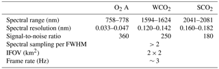
As illustrated by Kuang et al. (2002) and Crisp et al. (2004), three bands in the visual and near-infrared solar-reflected spectra are required to accurately measure atmospheric CO₂ and to efficiently eliminate the impacts of aerosols and clouds (Cressie et al., 2016). Table 1 shows a summary of the ACGS spectral requirements, including the spectral ranges and resolutions. The spectral regions shown in Table 1 are selected because these regions are relatively free of absorption by other gases. High-spectral resolutions can yield greater sensitivity while providing a low signal-to-noise ratio (SNR). In order to have a high SNR and a spectral sampling of more than two detector elements per FWHM, the spectral resolutions in the two CO₂ bands are slightly lower than that of the OCO-2.

2.2 Basic optical components of the ACGS

The ACGS consisted of a pointing mirror, a telescope system, beam splitters, focusing systems, slits, a collimating lens, plane gratings, and focal plane imaging systems. The pointing mirror, which is mounted on a one-dimensional rotation mechanism, is a specially designed optical element with two sides: the front side was designed and processed to be a mirror for reflecting the earthshine spectrum to the telescope, and the rear side was designed and prepared by physical grinding and chemical etching to be a 90 % reflecting diffuser for on-board solar calibration.

The optical design of the telescope system was based on a coaxial double parabolic crossed planar optical system with a beam contraction ratio of 3:2. A linear polarizer was placed in front of the slit of each spectrometer. The reflected light from the fore-optics system reaches the entrance slits of three spectrometers after being split, converged, and polarized by the beam splitters, condenser lenses, and polarizers, respectively. In each spectrometer, the light from the slit is collimated and directed to the plane grating. The image of the slit is formed on the focal plane array after diffracted light passes through the optical imaging system.

The spectral range in which the three spectrometers (which use three specifically designed holographic plane gratings in different bands) are arranged is as follows: the O₂ A-band (758–778 nm), the weak CO₂ band (1594–1624 nm), and the strong CO₂ band (2041–2081 nm). A folding mirror is used instead of the beam splitter for the last strong CO₂ band. The spectral dispersion of each spectrometer is mainly determined by the holographic plane grating used for each measured spectral band. In order to reduce the effect of stray light, a narrow-band isolation filter is placed between the beam splitter and condenser lens for the O₂ A-band, and the filters are placed in front of the detectors for the weak and strong CO₂ bands in the ACGS. To compensate for aberration, to correct the smile effect, and to square the slit image on the focal plane, a slightly curved entrance slit is used for each spectrometer. Since an increase in the area of the detector can effectively improve the SNR for an optical system with a fixed relative aperture, the detector-merging method is employed in the ACGS. In the spatial dimension, a certain number of detectors are combined into one to meet the ground resolution requirement of 2 km ×2 km.

3 Methodology

For high-spectral resolution spectrometers, there are many spectral calibration methods that are based on the use of quasi-monochromatic stimuli spectral light sources, gas absorption cells, atomic emission lines, tunable lasers, and solar spectra (Day and O'Dell, 2011; Gaiser et al., 2003). The tunable laser method has the advantage of high precision. We established the configuration including a tunable diode laser and wavemeter in our spectral calibration of TanSat. The tunable laser method requires waiting for frequency and intensity stabilization; thus, it is time consuming. In order to improve the efficiency of the spectral calibration, we devised an automatic measurement device that can continuously measure and scan the spectrum without manual intervention.

3.1 Laboratory testing equipment

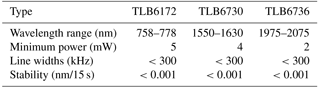
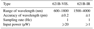
Determining the ILS for each spectral channel, footprint, and band was the central challenge of the ACGS spectral calibration. In the ACGS, there are 20178 individual ILS functions in the three bands in total. For OCO and OCO-2, only portions of the ILS functions were directly scanned (Day and O'Dell, 2011; Lee et al., 2017), while the other ILS functions were calculated by polynomial ILS interpolation across spectral bands in order to reduce the amount of time-consuming work. In this study, except for a very small 7 nm region of the SCO₂ band, all of the ILS profiles of the ACGS were scanned directly by three tunable diode lasers without any gaps in the range of each band. The lasers had a very narrow line width (<300 kHz), and the step size was 2 orders of magnitude smaller than the FWHM in each band. The stability of the laser at the desired wavelength was better than 5 pm, but tens of seconds were required to stabilize it. Table 2 shows the key parameters of the tunable laser. A wavemeter with an accuracy of 0.2 pm, manufactured by the Bristol Instrument Company, was used to monitor the laser wavelength accuracy and stability. Table 3 shows the relevant parameters of the wavemeter. Laser speckle can severely affect the light on the focal plane and cause random fluctuations in the final ILS functions. Laser speckle was removed using a spinning ground glass disk while reducing the laser intensity by approximately 20 %.

Table 2 Summary of the tunable diode laser parameters.

Figure 1 Schematic diagram of the ACGS spectral calibration.

Table 3 Summary of the wavemeter parameters.

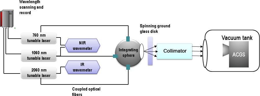
The laboratory setup and the schematic diagram of the ACGS spectral calibration are presented in Fig. 1. An automatic ILS measurement device was devised in this work. The device consists of a tunable diode laser, which was fiber coupled to both a wavemeter and a 5.08 cm Labsphere integrating sphere, collimator, and programming control system. This device can scan the spectrum and confirm the stability of the wavelength and intensity automatically according to specified settings. This system remarkably improved the measurement efficiency.

3.2 Data processing procedure

The scan range of the tunable diode laser used to determine detailed characterizations of single ILS functions was greater than ±5 FWHMs. By averaging tens of frames, some random noise in the laser and detector can be eliminated. After the whole range of each band is scanned, the raw ILS profiles for each channel can be generated. The centroid wavelength response of each channel can be found by the Gaussian fits to the raw ILS profiles. Then, the spectral polynomial fits can be used to calculate the dispersion coefficients. The spectral resolution expressed in FWHMs can also be calculated and assessed. Figure 2 presents a flowchart of the data processing procedure to determine the ILS, resolution and dispersion coefficients for each channel in each band. Because each channel was scanned by a tunable diode laser, this processing method was used for all channels to analyze the spectral parameters.

Figure 2 Flowchart of the instrument spectral calibration data processing.

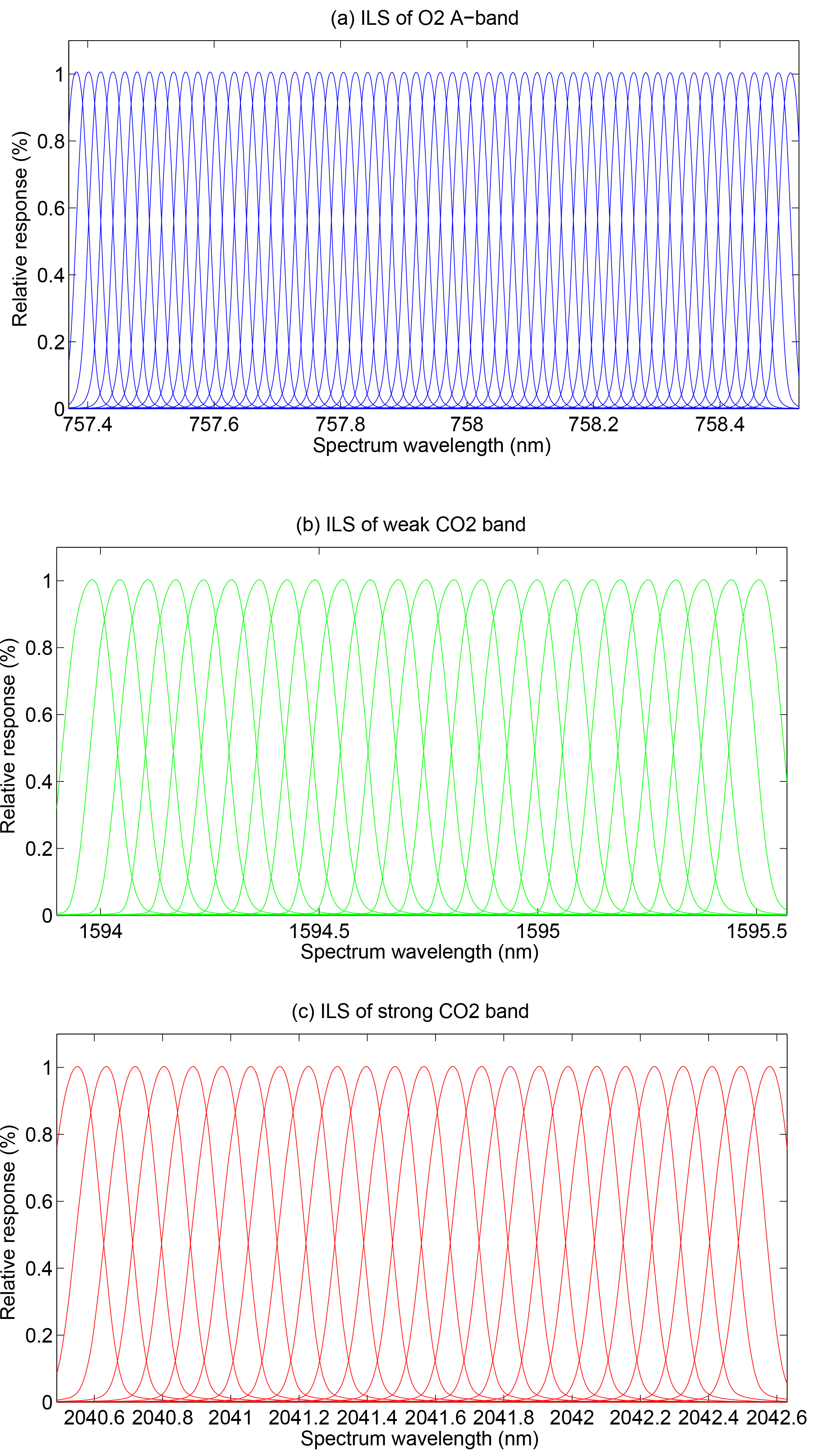
Figure 3 ILS of the first 60 channels in the O₂ A-band (a), and the first 25 channels in the WCO₂ (b) and the SCO₂ (c) bands of footprint 5.

Figure 4 The ILS bias between the center of footprint 5 and the other footprints in the first, center, and last channels in the three bands. The top row is the O₂ A-band, the middle row is the WCO₂ band, and the bottom row is the SCO₂ band. The left column is the first channel in the three bands, the middle column is the center channel, and the right column is the last channel in the three bands. Different colors represent the ILS biases between footprint 5 and different footprints.

4 Results

4.1 ILS profile

The ILS profile, i.e., the spectral response function of each channel, is one of the core parameters of high-spectral resolution instruments. The shape and consistency of the ILS profiles in a band are two key characteristics that indicate the precision of the spectral calibration (Beirle et al., 2017; Sun et al., 2017).

As can be seen from Fig. 3, the ILSs of the first 60 channels of footprint 5 in the O₂ A-band, which ranges from 757.42 to 758.50 nm, the first 25 channels in the WCO₂ band, which ranges from 1594.0 to 1595.5 nm, and in the SCO₂ band, which ranges from 2040.54 to 2042.56 nm, are always noticeably symmetrical (better then 99.99 %) and perfectly consistent across these channels.

In order to evaluate the ILSs consistency in depth, we assumed the ILS profile of the center channel, i.e., channel 621 of footprint 5, as a standard for comparison with other footprints in the first, center, and last channels in the three bands. We selected those channels at the center and both sides of detector because they can represent all of the channels of the detector. We call the variation of each point the ILS bias. As detailed in Fig. 4, there is a very small ILS bias in the spatial and spectral dimensions in the three bands. The ILS bias between the profiles of channel 621 of footprint 5 and the other footprints of the O₂ A-band was −0.0052 % to 0.0071 % in channel 1; less than ±0.005 % and more symmetrical in channel 621; and −0.029 % to 0.012 % in channel 1242, i.e., the last channel. The ILS biases between footprint 5 and other footprints of the WCO₂ band are −0.0066 % to 0.0127 % in channel 1; −0.009.8 % to 0.0072 % in channel 250; and −0.0155 % to 0.0074 % in channel 500, i.e., the last channel in WCO₂. There is noticeable symmetry in the ILS results for the WCO₂ band. The ILS biases between footprint 5 and the other footprints of the SCO₂ band are −0.0041 % to 0.0033 % in channel 1; −0.0053 % to 0.0029 % in channel 250; and −0.0183 % to 0.0145 % in last channel, which is perfectly consistent with previous results. The worst cases of consistency are better then 99.97 %, 99.98 %, and 99.98 % in the O₂A, WCO₂, and SCO₂ bands, respectively.

4.2 Spectral dispersion

OCO-1 and OCO-2 have completed very comprehensive works regarding spectral dispersion (Day and O'Dell, 2011; Lee et al., 2017). However, we also present spectral dispersion results, as seen in Fig. 5. The spectral dispersion coefficients observed in this study have excellent consistency in the nine footprints of each band and exhibit very good linearity in the spectral dimension of each band. A fifth-order polynomial fitting method is sufficient to model the tunable diode laser dispersion in each band, and the RMS errors of the fitting residuals are 0.9, 1, and 0.7 pm in theO₂ A-band, the WCO₂ band, and the SCO₂ band, respectively. These errors are negligible. In fact, only the first three low-order items of the fitted multinomial coefficients are significant; the other two high-order items are not significant.

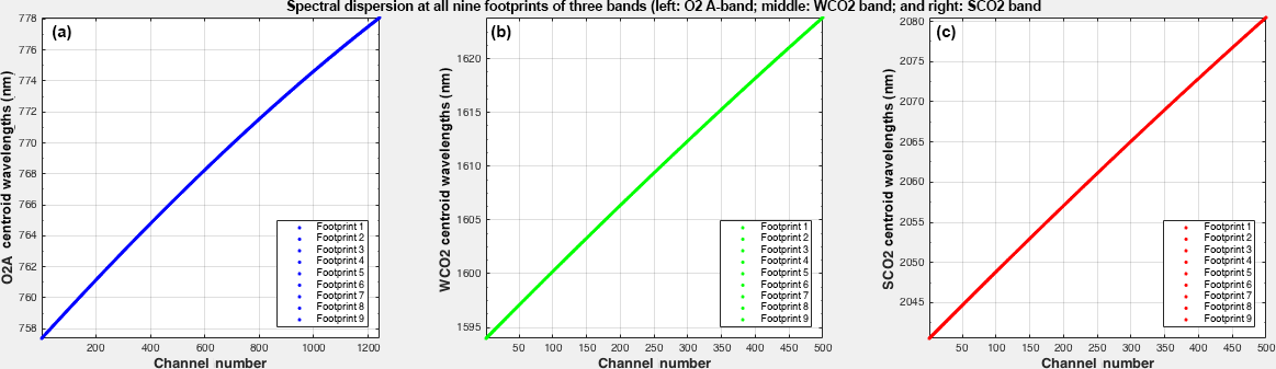
Figure 5 The spectral dispersion at all nine footprints of the three bands: the O₂ A-band (a), the WCO₂ band (b), and the SCO₂ band (c).

We summed the ILS profile variation in the comparisons above to obtain the area variation in the ILS profile. This measure can be thought of as the spectral response variation between footprint 5 and the other footprints in the spatial dimension. The maximum response variations are as follows: 0.5 %, 0.09 %, and −1.62 % in the first, middle, and last channels in the O₂ A-band; 0.63 %, 0.38 %, and −0.52 % in the first, middle, and last channel in the WCO₂ band; and 0.21 %, −0.15 %, 0.33 % in the first, middle, and last channel in the SCO₂ band, respectively. On the whole, the consistency of the ILS values across the spatial and spectral dimensions is perfect in the three bands. Most of the ILS response variations are less than 0.63 %. The maximum ILS variation was −1.62 % in last channel of the O₂ A-band between footprint 1 and footprint 5. Most of the bias is present at both wings of the ILS profiles and is negligible at the centroid wavelength of the ILS. Thus, the ILS variations resulting in changes in radiometric response and spectral dispersion are of little significance.

4.3 FWHM

The FWHM can be used to identify the spectral resolution of hyper-spectrometers. The FWHM was calculated from the ILS values for each channel in the three bands. The FWHMs for all channels are between 0.0393 and 0.0422 nm in the O₂ A-band, 0.123 and 0.128 nm in the WCO₂ band, and 0.16 and 0.17 nm in the SCO₂ band. Thus, the spectral resolving power (λ∕Δλ) values are ∼19 000, ∼12 800, and ∼12 250 in the O₂ A-band, the WCO₂ band, and the SCO₂ band, respectively, which indicates that the spectral resolution meets the mission requirements.

5 Conclusions

The spectral calibration of a super-high-resolution spectrometer is a big challenge due to the rigid precision requirements and the time-consuming nature of the work. In this study, we devised an elaborate automatic spectral calibration measurement device. The response of each channel of the ACGS was directly and automatically measured by a device that combines a tunable diode laser and a wavemeter, and this device, which was designed and implemented during this work, performs measurements without gaps in the spectral range of each band except for the last 7 nm in the longer wavelengths of the SCO₂ band. Values for these 7 nm were extrapolated from laser measurements of the first 33 nm of the SCO₂ band. Based on these data measured by lasers, we calculated and evaluated the ILS, FWHM, and spectral dispersion in each channel of the three bands. The ILSs were detailed in a previous section and were noticeably symmetrical and perfectly consistent across all channels in the three bands. The variation in the ILS resulted in negligible errors in the radiometric response and spectral calibrations. The FWHM characterization meets the mission requirements. The spectral dispersion had excellent consistency in the spatial dimension of each band and had good linearity in the spectral dimension of each band. Taken together, these results suggest that the ACGS spectral characterization meets the mission requirements. These characterizations will be evaluated again during the TanSat checkout on orbit, and the data will be validated using other similar space-based measurements.